HAL Id: hal-02999690
https://hal.archives-ouvertes.fr/hal-02999690
Submitted on 11 Nov 2020
HAL is a multi-disciplinary open access
archive for the deposit and dissemination of
sci-entific research documents, whether they are
pub-lished or not. The documents may come from
teaching and research institutions in France or
abroad, or from public or private research centers.
L’archive ouverte pluridisciplinaire HAL, est
destinée au dépôt et à la diffusion de documents
scientifiques de niveau recherche, publiés ou non,
émanant des établissements d’enseignement et de
recherche français ou étrangers, des laboratoires
publics ou privés.
The CFHQSIR survey: a Y-band extension of the
CFHTLS-Wide survey
S. Pipien, S. Basa, J.-G. Cuby, J.-C. Cuillandre, C. Willott, T. Moutard, J.
Chatron, S. Arnouts, P. Hudelot
To cite this version:
S. Pipien, S. Basa, J.-G. Cuby, J.-C. Cuillandre, C. Willott, et al.. The CFHQSIR survey: a Y-band
extension of the CFHTLS-Wide survey. Astronomy and Astrophysics - A&A, EDP Sciences, 2018,
616, pp.A55. �10.1051/0004-6361/201731944�. �hal-02999690�
Astronomy
&
Astrophysics
A&A 616, A55 (2018)
https://doi.org/10.1051/0004-6361/201731944 © ESO 2018
The CFHQSIR survey: a Y-band extension
of the CFHTLS-Wide survey
?
S. Pipien
1, S. Basa
1, J.-G. Cuby
1, J.-C. Cuillandre
2, C. Willott
3, T. Moutard
4, J. Chatron
1, S. Arnouts
1, and P. Hudelot
51 Aix-Marseille Université, CNRS, LAM, Laboratoire d’Astrophysique de Marseille, Marseille, France
e-mail: sarah.pipien@lam.fr
2 CEA/IRFU/SAp, Laboratoire AIM Paris-Saclay, CNRS/INSU, Université Paris Diderot, Observatoire de Paris, PSL Research
University, 91191 Gif-sur-Yvette Cedex, France
3 NRC Herzberg, 5071 West Saanich Rd, Victoria, BC V9E 2E7, Canada
4 Department of Astronomy & Physics and Institute for Computational Astrophysics, Saint Mary’s University, 923 Robie Street,
Halifax, Nova Scotia, B3H 3C3, Canada
5 Institut d’Astrophysique de Paris, 98bis Boulevard Arago, 75014 Paris, France
Received 13 September 2017 / Accepted 31 March 2018
ABSTRACT
Context. The Canada–France–Hawaii Telescope Legacy Survey (CFHTLS) has been conducted over a 5-yr period at the CFHT with
the MegaCam instrument, totaling 450 nights of observations. The Wide Synoptic Survey is one component of the CFHTLS, covering 155 square degrees in four patches of 23 to 65 square degrees through the whole MegaCam filter set (u*, g’, r’, i’, z’) down to i’AB=
24.5.
Aims. With the motivation of searching for high-redshift quasars at redshifts above 6.5, we extend the multi-wavelength
CFHTLS-Wide data in the Y-band down to magnitudes of ∼22.5 for point sources (5σ) .
Methods. We observed the four CFHTLS-Wide fields (except one quarter of the W3 field) in the Y-band with the Wide-field InfraRed
Camera (WIRCam) at the CFHT. Each field was visited twice, at least three weeks apart. Each visit consisted of two dithered exposures. The images are reduced with the Elixir software used for the CFHTLS and modified to account for the properties of near-InfraRed (IR) data. Two series of image stacks are subsequently produced: four-image stacks for each WIRCam pointing, and one-square-degree tiles matched to the format of the CFHTLS data release. Photometric calibration is performed on stars by fitting stellar spectra to their CFHTLS photometric data and extrapolating their Y-band magnitudes.
Results. After corrections accounting for correlated noise, we measure a limiting magnitude of YAB' 22.4 for point sources (5σ) in an
aperture diameter of 0.0093, over 130 square degrees. We produce a multi-wavelength catalogue combining the CFHTLS-Wide optical
data with our CFHQSIR (Canada–France High-z quasar survey in the near-InfraRed) Y-band data. We derive the Y-band number counts and compare them to the Vista Deep Extragalactic Observations survey (VIDEO). We find that the addition of the CFHQSIR Y-band data to the CFHTLS optical data increases the accuracy of photometric redshifts and reduces the outlier rate from 13.8% to 8.8% in the redshift range 1.05 . z . 1.2.
Key words. methods: data analysis – techniques: image processing – techniques: photometric – galaxies: photometry – infrared: general
1. Introduction
The Canada–France–Hawaii Telescope Legacy Survey (CFHTLS) has been conducted from mid-2003 to early 2009 at the CFHT (Canada–France–Hawaii Telescope) using the MegaCam wide field imaging camera, and totaling 450 nights (2300 h) of observations. MegaCam is a 1◦× 1◦ field of view
340 megapixels camera (Boulade et al. 2003) installed at the prime focus of the 3.6 m CFH telescope.
The CFHTLS consists of three distinct survey components: the supernovae and deep survey (SNLS and the Deep Survey), a wide synoptic survey (the Wide Survey) and a very wide shallow
?The CFHQSIR catalogue for 8.6 million sources down to
[(z0 ≤ 23.5) ∨ (Y ≤ 23.0)] is available at the CDS via anonymous
ftp tocdsarc.u-strasbg.fr(130.79.128.5) or via
http://cdsarc.u-strasbg.fr/viz-bin/qcat?J/A+A/616/A55. It is also available, as well as the Y-band images, at:
http://apps.canfar.net/storage/list/cjw/cfhqsir.
survey (the Very Wide Survey). The Wide Survey covers 155 square degrees in four patches of 23 to 65 square degrees through the whole filter set (u*, g’, r’, i’, z’) down to an AB magnitude i’ = 24.5.
As part of a large programme aimed at searching for quasars at redshifts of ∼7, we carried out Y-band near-IR observations of the CFHTLS-Wide Survey. This survey is intended to extend to higher redshifts the highly successful 5.8 < z < 6.5 Canada-France Quasar Survey (Willott et al. 2007,2009, 2010), from which our survey takes its name – CFHQSIR.
This data paper describes the CFHQSIR data. In the next section, we describe the survey observations. In Sect. 3, we present the data pre-processing, the photometric calibration and the CFHQSIR data format. In Sect.4we discuss the main proper-ties of the CFHQSIR data in terms of image quality and limiting magnitude. Section 5 addresses preliminary analyses (number counts and photometric redshifts) regarding the CFHQSIR data and the added value of the Y-band magnitude.
A55, page 1 of11
Open Access article,published by EDP Sciences, under the terms of the Creative Commons Attribution License (http://creativecommons.org/licenses/by/4.0), which permits unrestricted use, distribution, and reproduction in any medium, provided the original work is properly cited.
A&A 616, A55 (2018) A&A proofs: manuscript no. paper
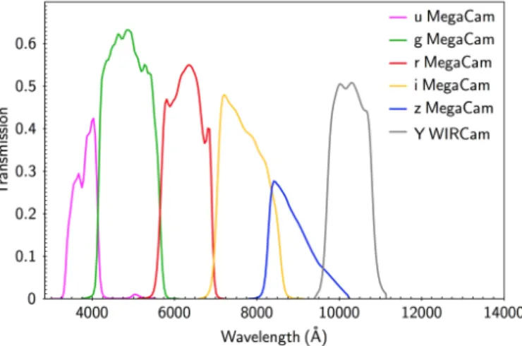
Fig. 1: Instrument and telescope total efficiency (optics and de-tector) in the MegaCam u*, g’, r’, i’, z’ filters and WIRCam Y-band.
WIRCam is mounted at the prime focus of the 3.6m CFH telescope. It is equipped with an image stabilization unit, which consists of a tip-tilt glass plate in front of the camera activated by the signal read-out from small 14×14 pixel regions centred on bright stars (Puget et al. 2004). The camera cryostat includes the eight-lens field corrector and an entrance window. The detector focal plane consists of a mosaic of four 2k × 2k HAWAII2-RG detectors separated by 7 mm. The sampling on sky is 000.3 per
18 µm pixel, providing a total field of view of 200× 200with a 2 0wide central cross between the four detectors.
The transmission curve of the Y-band filter used in this work is shown on Fig.1, together with the MegaCam filter transmis-sion curves.
The survey observations consisted of four dithered 75-seconds Y-band images of the same field. They were split into two visits, with dithering within a visit and between visits of 200.
The two visits were separated by at least 20 days in order to discard slow moving objects and strongly variable objects. The time difference between visits of the same field varied strongly between the four CFHTLS fields. For W1 and W4, the observa-tions were performed very rapidly at the beginning of the survey, while for W2 and W3 (winter and spring fields), they suffered from poorer weather conditions and were executed over much longer periods of time. The interval between visits of the same fields were in the range of 20-40 days for 50% (W1) and 90% (W4) of the observations, whereas for the W2 and W3 fields, most of the visits were separated by approximately one year.
The mapping of the fields was organized so as to match the CFHTLS one-square-degree tiles, with nine WIRCam pointings per CFHTLS tile. The observations were defined so as to pre-vent the execution of the second-visit observations in the same sequence as for the first visits, which could have generated sim-ilar persistence patterns in the data.
A total of approximately 150 hours of observations were conducted during four CFHT semesters, 2010B, 2011B, 2012A, and 2012B. The observations were carefully checked by our team in the days following the observations using the Elixir-IR pre-processing package (see next section), and observations that were executed under high background conditions and/or poor seeing conditions were not validated and were subsequently re-executed.
3. Data processing
3.1. Need for a custom pipeline: Elixir-IR
The CFHT offers to all its WIRCam users a data detrending and calibration service, the ‘I‘iwi pipeline (Thanjavur et al. 2011), which aims to remove the instrumental signature and delivers an absolute photometric calibration within 5%. This pipeline relies on generic recipes such as acquiring flat fields over a whole ob-serving run in order to create master detrending frames that are applied to all frames acquired during that observing period. This pipeline is directly derived and inspired from the earlier Elixir pipeline (Magnier & Cuillandre 2004) developed at the CFHT for its workhorse wide field imaging instrument operating in the visible domain, MegaCam. However, experience with Elixir has shown that particular attention to effects such as illumination and stability of the photometric response (Regnault et al. 2009) is re-quired when ultimate photometric stability is sought.
We therefore initiated a study of the stability in time of the WIRCam data. With an objective of a few percent photomet-ric accuracy across the field of view, an average flat field gath-ered over a seven to 15 day period was found clearly inadequate since the instrument exhibits changes in its response from night to night and especially from twilight to night. Indeed, dividing flat fields acquired over several days clearly shows residuals at small and large scales at the 5% level. These residuals affect the photometry at both medium and large scales.
Since ground-based near-IR observations are quickly sky-background-dominated, even in the Y-band CFHQSIR short ex-posures, it is possible to build flat-field frames directly from the science data over reasonably short timescales, thereby limiting the effects of instrumental variations over days. We therefore de-veloped a dedicated version of the Elixir pipeline, called Elixir-IR, aimed at minimizing the specifics of the WIRCam detectors, and more generally of near-IR detectors. The various processing steps are described in the following sub-sections.
3.2. Detector and raw data properties
A single 2048 × 2048 pixel detector array is read out through 32 outputs (Puget et al. 2004) in less than four seconds. The array is surrounded on the left, right, top and bottom by four columns and four lines of reference pixels, which do not integrate light and that are used to calibrate the additive level in the image signal (pedestal) as well as gradients and reset level from column to column, as described below.
A close inspection of a raw image uniformly illuminated shows important features that need to be accounted for, ei-ther by masking pixels that are not suitable for science, or by proper detrending with additive, non-linearity, and mul-tiplicative corrections (see Fig.2). We list here the major fea-tures: a) each readout amplifier has its own electronic operating properties leading to different gains (32 horizontal bands), b) the pixel reference pedestal can be sampled on the pixels on the left and right of the array, c) WIRCam using on-chip guiding, the pixels in the guide box (20 × 20 pixels) must be rejected from the scientific analysis1, d) the quantum efficiency shows
varia-tions, even scratches, across the surface, a result of the manu-facturing process, e) there are non-responsive pixels across all detectors, either isolated or in clusters of varying sizes, f) the electronic reset noise when reading out the detector through the
1 The columns and rows aligned to the guiding window are, however,
not rejected. Article number, page 2 of 12
Fig. 1.Instrument and telescope total efficiency (optics and detector) in the MegaCam u*, g’, r’, i’, z’ filters and WIRCam Y-band.
2. The CFHQSIR observations
The Wide-field InfraRed Camera (WIRCam) is the near-IR mosaic imager at the CFHT, which has been in operation since November 2006. WIRCam complements the one-square-degree optical imager, MegaCam, which has been in operation at CFHT since 2003.
WIRCam is mounted at the prime focus of the 3.6 m CFH telescope. It is equipped with an image stabilization unit, which consists of a tip-tilt glass plate in front of the camera activated by the signal read-out from small 14 × 14 pixel regions centred on bright stars (Puget et al. 2004). The camera cryostat includes the eight-lens field corrector and an entrance window. The detector focal plane consists of a mosaic of four 2 × 2 k HAWAII2-RG detectors separated by 7 mm. The sampling on sky is 0.003 per
18 µm pixel, providing a total field of view of 200× 200 with a
20wide central cross between the four detectors.
The transmission curve of the Y-band filter used in this work is shown on Fig. 1, together with the MegaCam filter transmission curves.
The survey observations consisted of four dithered 75 s Y-band images of the same field. They were split into two vis-its, with dithering within a visit and between visits of 200. The
two visits were separated by at least 20 days in order to discard slow moving objects and strongly variable objects. The time dif-ference between visits of the same field varied strongly between the four CFHTLS fields. For W1 and W4, the observations were performed very rapidly at the beginning of the survey, while for W2 and W3 (winter and spring fields), they suffered from poorer weather conditions and were executed over much longer periods of time. The interval between visits of the same fields were in the range of 20–40 days for 50% (W1) and 90% (W4) of the obser-vations, whereas for the W2 and W3 fields, most of the visits were separated by approximately 1 yr.
The mapping of the fields was organized so as to match the CFHTLS one-square-degree tiles, with nine WIRCam point-ings per CFHTLS tile. The observations were defined so as to prevent the execution of the second-visit observations in the same sequence as for the first visits, which could have generated similar persistence patterns in the data.
A total of approximately 150 h of observations were con-ducted during four CFHT semesters, 2010B, 2011B, 2012A, and 2012B. The observations were carefully checked by our team in the days following the observations using the Elixir-IR pre-processing package (see next section), and observations that
were executed under high background conditions and/or poor seeing conditions were not validated and were subsequently re-executed.
3. Data processing
3.1. Need for a custom pipeline: Elixir-IR
The CFHT offers to all its WIRCam users a data detrending and calibration service, the “I”iwi pipeline (Thanjavur et al. 2011), which aims to remove the instrumental signature and delivers an absolute photometric calibration within 5%. This pipeline relies on generic recipes, such as acquiring flat fields over a whole observing run in order to create master detrending frames that are applied to all frames acquired during that observing period. This pipeline is directly derived and inspired from the earlier Elixir pipeline (Magnier & Cuillandre 2004) developed at the CFHT for its workhorse wide field imaging instrument operating in the visible domain, MegaCam. However, experience with Elixir has shown that particular attention to effects, such as illumination and stability of the photometric response (Regnault et al. 2009) is required when ultimate photometric stability is sought.
We therefore initiated a study of the stability in time of the WIRCam data. With an objective of a few percent photometric accuracy across the field of view, an average flat field gath-ered over a seven to 15-day period was found clearly inadequate since the instrument exhibits changes in its response from night to night and especially from twilight to night. Indeed, dividing flat fields acquired over several days clearly shows residuals at small and large scales at the 5% level. These residuals affect the photometry at both medium and large scales.
Since ground-based near-IR observations are quickly sky-background-dominated, even in the Y-band CFHQSIR short exposures, it is possible to build flat-field frames directly from the science data over reasonably short timescales, thereby limit-ing the effects of instrumental variations over days. We therefore developed a dedicated version of the Elixir pipeline, called Elixir-IR, aimed at minimizing the specifics of the WIRCam detectors, and more generally of near-IR detectors. The various processing steps are described in the following sub-sections. 3.2. Detector and raw data properties
A single 2048 × 2048 pixel detector array is read out through 32 outputs (Puget et al. 2004) in less than four seconds. The array is surrounded on the left, right, top, and bottom by four columns and four lines of reference pixels, which do not integrate light and that are used to calibrate the additive level in the image sig-nal (pedestal), as well as gradients and reset level from column to column, as described below.
A close inspection of a raw image uniformly illuminated shows important features that need to be accounted for, either by masking pixels that are not suitable for science, or by proper detrending with additive, non-linearity, and multiplicative cor-rections (see Fig. 2). We list here the major features: a) each readout amplifier has its own electronic operating properties leading to different gains (32 horizontal bands), b) the pixel ref-erence pedestal can be sampled on the pixels on the left and right of the array, c) WIRCam using on-chip guiding, the pix-els in the guide box (20 × 20 pixpix-els) must be rejected from the scientific analysis1, d) the quantum efficiency shows variations,
1 The columns and rows aligned to the guiding window are, however,
not rejected. A55, page 2 of11
S. Pipien et al.: The CFHQSIR survey: a Y-band extension of the CFHTLS-Wide survey S. Pipien et al.: The CFHQSIR survey: a Y-band extension of the CFHTLS-Wide survey
Fig. 2: WIRCam detector features. multiplexer causes a non-constant pedestal setting, seen as
verti-cal comb structures across the entire height of the image. In the following, we describe how each of those features is handled in the Elixir-IR pipeline per detector and in a time-sequential approach. The pipeline handles all four detectors in parallel in a similar fashion.
– Reset noise. A single reset signal is applied to the entire de-tector once all columns have been readout through the 32 am-plifiers (each readout stripe being 64 pixels high). There is a noise associated to this process and this sets a new pedestal for the next column readout, an effect than can be as high as 10 to 15 ADUs(Analog-to-Digital Units). This effect is clearly visible on low background frames. In practice, this reset noise is highly correlated over three to four columns. The four lines of reference pixels at the top and bottom of the array are equally affected and can be used to build a one-dimensional horizontal model that is subtracted to the entire image. Figure3shows an image with and without the refer-ence pixel correction.
– Frame pedestal. The four columns on the left and right of the detector, now corrected from the reset noise, show a con-stant level, an artificial pedestal set by the readout electronics to ensure that no signal ever gets to negative levels after dou-ble correlated sampling. On WIRCam this artificial level is set around 1,000 ADUs. A simple median of all pixels from those eight columns is subtracted.
– Dark current. The WIRCam cryostat keeps the detectors at very low temperature (80K) and the dark current of 0.8 electrons per second and per pixel is nearly negligible with respect to the typical sky background level in the Y-band. Although stable over time, the dark current is, however, strongly dependent on integration time. Dark frames at the exposure time of the CFHQSIR (75 seconds) were taken in dark conditions to produce high signal-to-noise dark frames to substract from the science data.
– Non-linearity. The gain, readout noise, non-linearity, and saturation limits of all four detectors were derived using the photon transfer function (Janesick 2001). The detector gains are of the order of 4.0 electron per ADU (all four are simi-lar within 0.2 electrons per ADU), the readout noise is equal to 28 electrons, and the saturation limit varies from 100,000 electrons to 160,000 electrons between detectors.
Fig. 3: Illustration of the reference pixel correction (top: without, bottom: with) for an image of the W4 field.
– Bad pixels. We took the approach of masking all pixels that have a strongly discrepant response relative to the average re-sponse of the arrays. We compared two high signal-to-noise flat-field frames, one with an integration time twice as long as the other. After scaling with the integration time and sub-traction of the two images, we rejected all pixels with a resid-ual deviating from zero by more than 1% of the signal. The final bad pixel count is of the order of 2% per detector. The windows used by WIRCam for on-chip guiding (400 pixels)
Article number, page 3 of 12
Fig. 2.WIRCam detector features.
even scratches, across the surface, a result of the manufacturing process, e) there are non-responsive pixels across all detectors, either isolated or in clusters of varying sizes, f) the electronic reset noise when reading out the detector through the multi-plexer causes a non-constant pedestal setting, seen as vertical comb structures across the entire height of the image.
In the following, we describe how each of those features is handled in the Elixir-IR pipeline per detector and in a time-sequential approach. The pipeline handles all four detectors in parallel in a similar fashion.
– Reset noise. A single reset signal is applied to the entire detector once all columns have been readout through the 32 amplifiers (each readout stripe being 64-pixels high). There is a noise associated to this process and this sets a new pedestal for the next column readout, an effect than can be as high as 10–15 analog-to-digital units (ADUs). This effect is clearly visible on low background frames. In practice, this reset noise is highly correlated over three to four columns. The four lines of reference pixels at the top and bottom of the array are equally affected and can be used to build a one-dimensional horizontal model that is subtracted to the entire image. Figure3shows an image with and without the reference pixel correction.
– Frame pedestal. The four columns on the left and right of the detector, now corrected from the reset noise, show a constant level, an artificial pedestal set by the readout electronics to ensure that no signal ever gets to negative levels after double correlated sampling. On WIRCam this artificial level is set around 1000 ADUs. A simple median of all pixels from those eight columns is subtracted.
– Dark current. The WIRCam cryostat keeps the detectors at very low temperature (80 K) and the dark current of 0.8 electrons per second and per pixel is nearly negligi-ble with respect to the typical sky background level in the Y-band. Although stable over time, the dark current is, how-ever, strongly dependent on integration time. Dark frames at the exposure time of the CFHQSIR (75 s) were taken in dark conditions to produce high signal-to-noise (S/N) dark frames to substract from the science data.
– Non-linearity. The gain, readout noise, non-linearity, and saturation limits of all four detectors were derived using the photon transfer function (Janesick 2001). The detector gains are of the order of 4.0 electron per ADU (all four are simi-lar within 0.2 electrons per ADU), the readout noise is equal
S. Pipien et al.: The CFHQSIR survey: a Y-band extension of the CFHTLS-Wide survey
Fig. 2: WIRCam detector features. multiplexer causes a non-constant pedestal setting, seen as
verti-cal comb structures across the entire height of the image. In the following, we describe how each of those features is handled in the Elixir-IR pipeline per detector and in a time-sequential approach. The pipeline handles all four detectors in parallel in a similar fashion.
– Reset noise. A single reset signal is applied to the entire de-tector once all columns have been readout through the 32 am-plifiers (each readout stripe being 64 pixels high). There is a noise associated to this process and this sets a new pedestal for the next column readout, an effect than can be as high as 10 to 15 ADUs(Analog-to-Digital Units). This effect is clearly visible on low background frames. In practice, this reset noise is highly correlated over three to four columns. The four lines of reference pixels at the top and bottom of the array are equally affected and can be used to build a one-dimensional horizontal model that is subtracted to the entire image. Figure3shows an image with and without the refer-ence pixel correction.
– Frame pedestal. The four columns on the left and right of the detector, now corrected from the reset noise, show a con-stant level, an artificial pedestal set by the readout electronics to ensure that no signal ever gets to negative levels after dou-ble correlated sampling. On WIRCam this artificial level is set around 1,000 ADUs. A simple median of all pixels from those eight columns is subtracted.
– Dark current. The WIRCam cryostat keeps the detectors at very low temperature (80K) and the dark current of 0.8 electrons per second and per pixel is nearly negligible with respect to the typical sky background level in the Y-band. Although stable over time, the dark current is, however, strongly dependent on integration time. Dark frames at the exposure time of the CFHQSIR (75 seconds) were taken in dark conditions to produce high signal-to-noise dark frames to substract from the science data.
– Non-linearity. The gain, readout noise, non-linearity, and saturation limits of all four detectors were derived using the photon transfer function (Janesick 2001). The detector gains are of the order of 4.0 electron per ADU (all four are simi-lar within 0.2 electrons per ADU), the readout noise is equal to 28 electrons, and the saturation limit varies from 100,000 electrons to 160,000 electrons between detectors.
Fig. 3: Illustration of the reference pixel correction (top: without, bottom: with) for an image of the W4 field.
– Bad pixels. We took the approach of masking all pixels that have a strongly discrepant response relative to the average re-sponse of the arrays. We compared two high signal-to-noise flat-field frames, one with an integration time twice as long as the other. After scaling with the integration time and sub-traction of the two images, we rejected all pixels with a resid-ual deviating from zero by more than 1% of the signal. The final bad pixel count is of the order of 2% per detector. The windows used by WIRCam for on-chip guiding (400 pixels)
Article number, page 3 of 12
Fig. 3. Illustration of the reference pixel correction (top: without, bottom: with) for an image of the W4 field.
to 28 electrons, and the saturation limit varies from 100 000 electrons to 160 000 electrons between detectors.
– Bad pixels. We took the approach of masking all pixels that have a strongly discrepant response relative to the average response of the arrays. We compared two high S/N flat-field frames, one with an integration time twice as long as the other. After scaling with the integration time and subtraction of the two images, we rejected all pixels with a residual devi-ating from zero by more than 1% of the signal. The final bad pixel count is of the order of 2% per detector. The windows used by WIRCam for on-chip guiding (400 pixels) are also treated as bad pixels on an image by image basis by Elixir-IR.
A&A 616, A55 (2018)
– Building a flat field. Near-IR observations are characterized by strong spatial and temporal sky variations (OH airglow), as well as detector property variations (e.g., gain) over time, possibly due to controller temperature variations. Building appropriate flat fields therefore requires caution.
We initially performed a number of tests to check the stability of the illumination pattern over time. We found that there are gain drifts of ≈1% over timescales of the order of three hours. This makes the use of twilight flat fields inap-propriate, not considering the strong spatial variations of the twilight flat-field patterns which can exceed 5% over short timescales. In order to limit the gain variations to well below 1%, we adopted time windows of the order of 30 min to generate sky flat fields.
Considering the CFHQSIR observing strategy, and including readout and telescope pointing overheads, 14 expo-sures (seven dithered pairs of 75 s each) fit within an ≈20 min long time window. The signal is largely dominated by the high sky background (typically 2000–5000 ADUs); 14 exposures on seven independent pointings are therefore, adequate to derive good flat fields. The flat-field frames are generated by averaging the 14 frames with iterative sigma clipping making use of the detector gain and noise prop-erties. We note that including the central science frame in the flat-fielding procedure can introduce a photometric bias, depending on the averaging method. This bias can be as high as the inverse of the number of frames when using a simple median. However, with our iterative image rejection method based on photon noise properties, the bias shrinks to negligible levels (less than 1 %).
3.3. Inspection and stacking
After removal of the detector features and flat-fielding, the images are free of cosmetics patterns. The main remaining pat-terns are cosmic rays and low frequency background residuals (tilts) that are due to the structure of the OH airglow and to its evolution over time. Except for these residuals, all features on the science images are flattened at the 0.1% level (min.–max.), comparable to what is achieved on CCDs using the Elixir-LSB pipeline on MegaCam data.
Once the individual frames are fully detrended, they are visually inspected through a quick preview procedure to check the images look fine and in particular if the sky background (airglow) has a normal behavior, changing in subtle ways from one exposure to the next (see bottom image of Fig. 3 for an illustration of the typical appearance of an Elixir-IR detrended frame, all four detectors being normalized to the same response). Individual frames are then calibrated for astrometry using the Two Micron All Sky Survey (2MASS) catalogue (Skrutskie et al. 2006).
For stacking, we adopt the AstrOmatic suite2 by E. Bertin
to derive a fine astrometry (SCAMP) and resample the images for alignment on a given grid and stacking (SWarp). The sky background is subtracted as two-dimensional (2D) plane fits to individual images. In most cases, stacks consist of four images. Despite this small number of data points, good rejection of bad pixels, cosmic rays, and spurious signals is achieved with sigma-clipping using the detector noise parameters (gain and noise). Remnant signals from previous observations of heavily saturated stars are mostly removed during this stacking process but can be easily identified on averaged stacks. If the remnant originates
2 www.astromatic.net
A&A proofs: manuscript no. paper
are also treated as bad pixels on an image by image basis by Elixir-IR.
– Building a flat field. Near IR observations are characterized by strong spatial and temporal sky variations (OH airglow), as well as detector property variations (e.g. gain) over time, possibly due to controller temperature variations. Building appropriate flat fields therefore requires caution.
We initially performed a number of tests to check the sta-bility of the illumination pattern over time. We found that there are gain drifts of ≈ 1% over timescales of the order of three hours. This makes the use of twilight flat fields inap-propriate, not considering the strong spatial variations of the twilight flat-field patterns which can exceed 5% over short timescales. In order to limit the gain variations to well below 1%, we adopted time windows of the order of 30 minutes to generate sky flat fields.
Considering the CFHQSIR observing strategy, and includ-ing readout and telescope pointinclud-ing overheads, 14 exposures (seven dithered pairs of 75s each) fit within an ≈ 20 minute long time window. The signal is largely dominated by the high sky background (typically 2000 to 5000 ADUs) ; 14 exposures on seven independent pointings are therefore ad-equate to derive good flat fields. The flat-field frames are generated by averaging the 14 frames with iterative sigma clipping making use of the detector gain and noise proper-ties. We note that including the central science frame in the flat-fielding procedure can introduce a photometric bias, de-pending on the averaging method. This bias can be as high as the inverse of the number of frames when using a simple median. However, with our iterative image rejection method based on photon noise properties, the bias shrinks to negligi-ble levels (less than 1 %).
3.3. Inspection and stacking
After removal of the detector features and flat-fielding, the im-ages are free of cosmetics patterns. The main remaining patterns are cosmic rays and low frequency background residuals (tilts) that are due to the structure of the OH airglow and to its evolution over time. Except for these residuals, all features on the science images are flattened at the 0.1% level (min-max), comparable to what is achieved on CCDs using the Elixir-LSB pipeline on MegaCam data.
Once the individual frames are fully detrended, they are vi-sually inspected through a quick preview procedure to check the images look fine and in particular if the sky background (air-glow) has a normal behavior, changing in subtle ways from one exposure to the next (see bottom image of Fig.3for an illustra-tion of the typical appearance of an Elixir-IR detrended frame, all four detectors being normalized to the same response). Indi-vidual frames are then calibrated for astrometry using the Two Micron All Sky Survey (2MASS) catalogue (Skrutskie et al. 2006).
For stacking, we adopt the AstrOmatic suite2 by E. Bertin
to derive a fine astrometry (SCAMP) and resample the images for alignment on a given grid and stacking (SWarp). The sky background is subtracted as two-dimensional (2D) plane fits to individual images. In most cases, stacks consist of four images. Despite this small number of data points, good rejection of bad pixels, cosmic rays, and spurious signals is achieved with sigma-clipping using the detector noise parameters (gain and noise). Remnant signals from previous observations of heavily saturated
2 www.astromatic.net
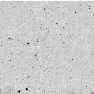
Fig. 4: Image of one quadrant of a WIRCam stack in the W4 field produced by the Elixir-IR pipeline.
stars are mostly removed during this stacking process but can be easily identified on averaged stacks. If the remnant originates from an image recorded earlier in the night and unrelated to CFHQSIR, the persistence pattern consists of two spots along the dither direction, whereas the pattern has three spots if the remnant originates from a dithered pair of previous CFHQSIR observations. Due to the small offsets between images, it was not necessary to apply illumination correction (see next section) before stacking. Weight maps for each stack are also produced by SWarp during the resampling and stacking process. An ex-ample is shown in Fig. 4. These weight maps include the 2 0
gaps between the four detector arrays. The four-image stacks so produced will be referred to in the following as WIRCam stacks.
3.4. Photometric calibration
Information on photometric calibration in the Y-band is scarce due to the limited use of this band. Direct photometric cali-bration of the Y-band using Vega-like A0 stars has been per-formed by for example Hillenbrand et al.(2002). The Y-band UKIDSS (UKIRT Infrared Deep Sky Survey) - WFCAM (Wide Field Camera) data were anchored to the Two-Micron All-Sky Survey (2MASS) and calibrated in the Vega system by zeroing the colours of blue stars present in the data (Hodgkin et al. 2009). Considering the connection between the CFHQSIR and CFHTLS datasets, we chose to anchor the CFHQSIR photomet-ric calibration to the CFHTLS and to treat the Y-band extension as an extrapolation in wavelength. For convenience, we decided to perform the photometric calibration directly on the image stacks (WIRCam stacks) as described in the previous section. To this end, we select unsaturated and high signal-to-noise ratio (SNR) stars in our Y-band catalogue, and we fit stellar spectra to their griz magnitudes, making additional use, when available, of 2MASS JHK photometric data.
In more detail, we proceed as follows:
Article number, page 4 of 12
Fig. 4. Image of one quadrant of a WIRCam stack in the W4 field produced by the Elixir-IR pipeline.
from an image recorded earlier in the night and unrelated to CFHQSIR, the persistence pattern consists of two spots along the dither direction, whereas the pattern has three spots if the remnant originates from a dithered pair of previous CFHQSIR observations. Due to the small offsets between images, it was not necessary to apply illumination correction (see next section) before stacking. Weight maps for each stack are also produced by SWarp during the resampling and stacking process. An exam-ple is shown in Fig.4. These weight maps include the 20 gaps
between the four detector arrays. The four-image stacks so produced will be referred to in the following as WIRCam stacks.
3.4. Photometric calibration
Information on photometric calibration in the Y-band is scarce due to the limited use of this band. Direct photometric calibra-tion of the Y-band using Vega-like A0 stars has been performed by for exampleHillenbrand et al.(2002). The Y-band UKIDSS (UKIRT Infrared Deep Sky Survey) – WFCAM (Wide Field Camera) data were anchored to the Two-Micron All-Sky Sur-vey (2MASS) and calibrated in the Vega system by zeroing the colours of blue stars present in the data (Hodgkin et al. 2009).
Considering the connection between the CFHQSIR and CFHTLS datasets, we chose to anchor the CFHQSIR photomet-ric calibration to the CFHTLS and to treat the Y-band extension as an extrapolation in wavelength. For convenience, we decided to perform the photometric calibration directly on the image stacks (WIRCam stacks) as described in the previous section. To this end, we select unsaturated and high S/N stars in our Y-band catalogue, and we fit stellar spectra to their griz mag-nitudes, making additional use, when available, of 2MASS JHK photometric data.
In more detail, we proceed as follows:
– From our Y-band catalogue, we select unsaturated objects classified as stars by SExtractor and with an S/N matching
S. Pipien et al.: The CFHQSIR survey: a Y-band extension of the CFHTLS-Wide survey S. Pipien et al.: The CFHQSIR survey: a Y-band extension of the CFHTLS-Wide survey
Fig. 5: Example of a fit with a K-type spectrum in a case where 2MASS data are available. The derived Y-band magnitude is in-dicated by the circle.
1. From our Y-band catalogue, we select unsaturated objects classified as stars by SExtractor and with an SNR matching our target photometric accuracy of a few percent. In practice, we selected objects with SNR > 40.
2. We search for these stars in the CFHTLS catalogue within a 100search radius and we use the “IQ20" magnitudes,
follow-ing the prescription ofHudelot et al. (2012) for point-like objects. The CFHTLS “IQ20” magnitudes are the true to-tal magnitudes integrated over an aperture 20 times the full width at half maximum (FWHM) of the point spread func-tion (PSF).
3. When available, the 2MASS (profile-fitting) magnitudes in the J, H, and Ksbands are also used in the fits.
4. For each star, we fit the optical photometric data with the Pickles(1998) library of stellar spectra and we derive the Y-band magnitude from these fits. To this aim, we use the Le Phare (Arnouts et al. 1999;Ilbert et al. 2006) photometric redshift sofware.
5. We intentionally use a limited number of spectra represen-tative of the most common stars likely to be present in our samples, and we exclude cold stars that have broad absorp-tion features in the near-IR, therefore preventing a reliable extrapolation of their spectra. We therefore limit the spectral types used for our fitting procedure from G0 to K7. We also limit the photometric bands used in the fit to the riz[JHKs] bands to avoid the sensitivity to metallicity of the u and g bands. We exclude poor fits as measured by the Le Phare in-ternally derived χ2values.
An example of a fit with a stellar spectrum to the spectral energy distribution of a star for which there are ugriz CFHTLS and JHKs 2MASS photometry is shown in Fig.5. The u and g bands data points are shown but are not used in the fit. In total, we use 45,500 stars to perform this photometric calibration over the four CFHQSIR fields, leading to an average photometric zero point per quadrant (detector) of each WIRCam stack. We tenta-tively observe a less than 1% difference between the zero points derived with or without 2MASS data, not significant enough to be corrected for.
Fig. 6: Colour-coded flux calibration coefficients per star FZPas
a function of the star position in the WIRCam focal plane.The calibration coefficient FZPis defined as the ratio, before
calibra-tion, of the flux fitted with Le Phare to the flux measured by SExtractor.
Fig. 7: Map used to correct the spatial non-uniformity of the pho-tometric response. The peak-to-peak relative amplitude variation in this image is 20 %.
After this first pass the relative dispersion of the calibration coefficients is equal to 10%. This dispersion includes photomet-ric variations between stacks and spatial variations within one quadrant and between quadrants. Spatial variations of the zero points due to optical distortions and/or sky concentration are in-troduced during the flat-fielding process (see e.g.Regnault et al. 2009). These variations can be seen on Fig.6, which shows the zero points projected onto a single WIRCam image in pixel co-ordinates. From this image, we generate a 2D fit per quadrant (Fig.7), usually referred to as illumination-correction map. This map is subsequently used to correct all the WIRCam stacks.
After correction for the illumination map, we re-compute all the zero points for the whole dataset. For each WIRCam stack, we derived the final zero point by averaging with sigma-clipping rejection the zero points measured for each star present in the
Article number, page 5 of 12
Fig. 5.Example of a fit with a K-type spectrum in a case where 2MASS data are available. The derived Y-band magnitude is indicated by the circle.
our target photometric accuracy of a few percent. In practice, we selected objects with S/N > 40.
– We search for these stars in the CFHTLS catalogue within a 100 search radius and we use the “IQ20” magnitudes,
following the prescription ofHudelot et al.(2012) for point-like objects. The CFHTLS “IQ20” magnitudes are the true total magnitudes integrated over an aperture 20 times the full width at half maximum (FWHM) of the point spread function (PSF).
– When available, the 2MASS (profile-fitting) magnitudes in the J, H, and Ksbands are also used in the fits.
– For each star, we fit the optical photometric data with the Pickles (1998) library of stellar spectra and we derive the Y-band magnitude from these fits. To this aim, we use the LE
PHARE(Arnouts et al. 1999;Ilbert et al. 2006) photometric
redshift sofware.
– We intentionally use a limited number of spectra represen-tative of the most common stars likely to be present in our samples, and we exclude cold stars that have broad absorp-tion features in the near-IR, therefore preventing a reliable extrapolation of their spectra. We therefore limit the spec-tral types used for our fitting procedure from G0 to K7. We also limit the photometric bands used in the fit to the riz[JHKs] bands to avoid the sensitivity to metallicity of the u and g bands. We exclude poor fits as measured by the LE
PHAREinternally derived χ2values.
An example of a fit with a stellar spectrum to the spectral energy distribution of a star for which there are ugriz CFHTLS and JHKs 2MASS photometry is shown in Fig.5. The U and G bands data points are shown but are not used in the fit. In total, we use 45 500 stars to perform this photometric calibration over the four CFHQSIR fields, leading to an average photometric zero point per quadrant (detector) of each WIRCam stack. We tenta-tively observe a less than 1% difference between the zero points derived with or without 2MASS data, not significant enough to be corrected for.
After this first pass the relative dispersion of the calibration coefficients is equal to 10%. This dispersion includes photomet-ric variations between stacks and spatial variations within one quadrant and between quadrants. Spatial variations of the zero
S. Pipien et al.: The CFHQSIR survey: a Y-band extension of the CFHTLS-Wide survey
Fig. 5: Example of a fit with a K-type spectrum in a case where 2MASS data are available. The derived Y-band magnitude is in-dicated by the circle.
1. From our Y-band catalogue, we select unsaturated objects classified as stars by SExtractor and with an SNR matching our target photometric accuracy of a few percent. In practice, we selected objects with SNR > 40.
2. We search for these stars in the CFHTLS catalogue within a 100search radius and we use the “IQ20" magnitudes,
follow-ing the prescription of Hudelot et al. (2012) for point-like objects. The CFHTLS “IQ20” magnitudes are the true to-tal magnitudes integrated over an aperture 20 times the full width at half maximum (FWHM) of the point spread func-tion (PSF).
3. When available, the 2MASS (profile-fitting) magnitudes in the J, H, and Ksbands are also used in the fits.
4. For each star, we fit the optical photometric data with the Pickles(1998) library of stellar spectra and we derive the Y-band magnitude from these fits. To this aim, we use the Le Phare (Arnouts et al. 1999;Ilbert et al. 2006) photometric redshift sofware.
5. We intentionally use a limited number of spectra represen-tative of the most common stars likely to be present in our samples, and we exclude cold stars that have broad absorp-tion features in the near-IR, therefore preventing a reliable extrapolation of their spectra. We therefore limit the spectral types used for our fitting procedure from G0 to K7. We also limit the photometric bands used in the fit to the riz[JHKs] bands to avoid the sensitivity to metallicity of the u and g bands. We exclude poor fits as measured by the Le Phare in-ternally derived χ2values.
An example of a fit with a stellar spectrum to the spectral energy distribution of a star for which there are ugriz CFHTLS and JHKs 2MASS photometry is shown in Fig.5. The u and g bands data points are shown but are not used in the fit. In total, we use 45,500 stars to perform this photometric calibration over the four CFHQSIR fields, leading to an average photometric zero point per quadrant (detector) of each WIRCam stack. We tenta-tively observe a less than 1% difference between the zero points derived with or without 2MASS data, not significant enough to be corrected for.
Fig. 6: Colour-coded flux calibration coefficients per star FZPas
a function of the star position in the WIRCam focal plane.The calibration coefficient FZPis defined as the ratio, before
calibra-tion, of the flux fitted with Le Phare to the flux measured by SExtractor.
Fig. 7: Map used to correct the spatial non-uniformity of the pho-tometric response. The peak-to-peak relative amplitude variation in this image is 20 %.
After this first pass the relative dispersion of the calibration coefficients is equal to 10%. This dispersion includes photomet-ric variations between stacks and spatial variations within one quadrant and between quadrants. Spatial variations of the zero points due to optical distortions and/or sky concentration are in-troduced during the flat-fielding process (see e.g.Regnault et al. 2009). These variations can be seen on Fig.6, which shows the zero points projected onto a single WIRCam image in pixel co-ordinates. From this image, we generate a 2D fit per quadrant (Fig.7), usually referred to as illumination-correction map. This map is subsequently used to correct all the WIRCam stacks.
After correction for the illumination map, we re-compute all the zero points for the whole dataset. For each WIRCam stack, we derived the final zero point by averaging with sigma-clipping rejection the zero points measured for each star present in the
Article number, page 5 of 12
Fig. 6.Colour-coded flux calibration coefficients per star FZPas a
func-tion of the star posifunc-tion in the WIRCam focal plane.The calibrafunc-tion coefficient FZPis defined as the ratio, before calibration, of the flux fitted
with LEPHAREto the flux measured by SExtractor. S. Pipien et al.: The CFHQSIR survey: a Y-band extension of the CFHTLS-Wide survey
Fig. 5: Example of a fit with a K-type spectrum in a case where 2MASS data are available. The derived Y-band magnitude is in-dicated by the circle.
1. From our Y-band catalogue, we select unsaturated objects classified as stars by SExtractor and with an SNR matching our target photometric accuracy of a few percent. In practice, we selected objects with SNR > 40.
2. We search for these stars in the CFHTLS catalogue within a 100search radius and we use the “IQ20" magnitudes,
follow-ing the prescription of Hudelot et al. (2012) for point-like objects. The CFHTLS “IQ20” magnitudes are the true to-tal magnitudes integrated over an aperture 20 times the full width at half maximum (FWHM) of the point spread func-tion (PSF).
3. When available, the 2MASS (profile-fitting) magnitudes in the J, H, and Ksbands are also used in the fits.
4. For each star, we fit the optical photometric data with the Pickles(1998) library of stellar spectra and we derive the Y-band magnitude from these fits. To this aim, we use the Le Phare (Arnouts et al. 1999;Ilbert et al. 2006) photometric redshift sofware.
5. We intentionally use a limited number of spectra represen-tative of the most common stars likely to be present in our samples, and we exclude cold stars that have broad absorp-tion features in the near-IR, therefore preventing a reliable extrapolation of their spectra. We therefore limit the spectral types used for our fitting procedure from G0 to K7. We also limit the photometric bands used in the fit to the riz[JHKs] bands to avoid the sensitivity to metallicity of the u and g bands. We exclude poor fits as measured by the Le Phare in-ternally derived χ2values.
An example of a fit with a stellar spectrum to the spectral energy distribution of a star for which there are ugriz CFHTLS and JHKs 2MASS photometry is shown in Fig.5. The u and g bands data points are shown but are not used in the fit. In total, we use 45,500 stars to perform this photometric calibration over the four CFHQSIR fields, leading to an average photometric zero point per quadrant (detector) of each WIRCam stack. We tenta-tively observe a less than 1% difference between the zero points derived with or without 2MASS data, not significant enough to be corrected for.
Fig. 6: Colour-coded flux calibration coefficients per star FZPas
a function of the star position in the WIRCam focal plane.The calibration coefficient FZPis defined as the ratio, before
calibra-tion, of the flux fitted with Le Phare to the flux measured by SExtractor.
Fig. 7: Map used to correct the spatial non-uniformity of the pho-tometric response. The peak-to-peak relative amplitude variation in this image is 20 %.
After this first pass the relative dispersion of the calibration coefficients is equal to 10%. This dispersion includes photomet-ric variations between stacks and spatial variations within one quadrant and between quadrants. Spatial variations of the zero points due to optical distortions and/or sky concentration are in-troduced during the flat-fielding process (see e.g.Regnault et al. 2009). These variations can be seen on Fig.6, which shows the zero points projected onto a single WIRCam image in pixel co-ordinates. From this image, we generate a 2D fit per quadrant (Fig.7), usually referred to as illumination-correction map. This map is subsequently used to correct all the WIRCam stacks.
After correction for the illumination map, we re-compute all the zero points for the whole dataset. For each WIRCam stack, we derived the final zero point by averaging with sigma-clipping rejection the zero points measured for each star present in the
Article number, page 5 of 12
Fig. 7.Map used to correct the spatial non-uniformity of the photomet-ric response. The peak-to-peak relative amplitude variation in this image is 20 %.
points due to optical distortions and/or sky concentration are introduced during the flat-fielding process (see e.g., Regnault et al. 2009). These variations can be seen on Fig. 6, which shows the zero points projected onto a single WIRCam image in pixel coordinates. From this image, we generate a 2D fit per quadrant (Fig.7), usually referred to as illumination-correction map. This map is subsequently used to correct all the WIRCam stacks.
After correction for the illumination map, we re-compute all the zero points for the whole dataset. For each WIRCam stack, we derived the final zero point by averaging with sigma-clipping rejection the zero points measured for each star present in the stack. We require that a minimum of six zero points be measured in each stack. When there are less than six zero points, which happened for nine stacks only over a total of 1445), we assigned the average zeropoint of the corresponding CFHTLS field. For these nine stacks, this may represent an additional photometric error of less than 10%.
A&A 616, A55 (2018)
The illumination correction reduced the overall dispersion of the zero points from 10% to 7%, consistent with the amplitude of the illumination correction map. Finally, for consistency with the CFHTLS data (Hudelot et al. 2012), we normalize each stack by setting the zero point to a value of 30.0 in the AB system. 3.5. Registration to the CFHTLS format
For ease of use in connection with the CFHTLS data, we decided to produce one-square-degree image tiles similar to the CFHTLS data format, in addition to the WIRCam stacks. We use SCAMP (Bertin 2006) to determine the geometrical transfor-mation between the reference z-band CFHTLS tile and the nine WIRCam stacks corresponding to this tile. In practice, the trans-formation is determined for each of the four quadrants of the WIRCam stacks using a three-degree polynomial. We then use SWarp (Bertin et al. 2002) to apply these transformations using a LANCZOS3 (Lanczos-3 6-tap filter) interpolation kernel and to reformat the whole dataset to the CFHTLS tile format.
When there is overlap between adjacent WIRCam stacks within a tile, all the pixels in the overlapping regions are used. Conversely, pixels in overlaps between tiles3 are treated
independently.
4. Main properties of the survey
We present in this section the main properties of the CFHQSIR survey data. We perform the analysis either on the WIRCam stacks or on the one-square-degree images mapped into the CFHTLS format (tiles) described in the previous section. We fur-ther divide each tile into 3 × 3 sub-images corresponding to the footprint of each WIRCam stack.
4.1. Image quality
All observations were carried out in service mode, with an IQ constraint in the K-band of 0.0055 to 0.0065, which translates,
assuming a seeing limited image, to 0.0065 to 0.0075 in the Y-band.
This is very consistent with our measured image quality. Figure8 shows maps of the median image quality per sub-tile image mea-sured on unsaturated stars over the four CFHTLS fields. The number of stars used to determine the image quality was of the order of one hundred per sub-tile image. The histogram of the FWHM of all the stars used is represented in Fig.9.
We have explored the variation of the image quality over the WIRCam images. Figure10 shows the x and y position of all unsaturated stars used for the photometric calibration (see Sect.3.4). Despite the variations in seeing, one can note the spatial variations across the WIRCam field of view. The image quality is generally worse at the edge of the field. A region at the bottom left corner of the image shows very poor image qual-ity, attributed to detector issues since this region is adjacent to a region of very poor cosmetics and dead pixels. This bad quality region has been subsequently masked in the CFHQSIR data. 4.2. Sensitivity
4.2.1. Correlated noise correction
Image resampling introduces correlations in the noise that should be accounted for in the photometric error budgets. Discussions of this effect can be found for instance in
3 Adjacent CFHTLS tiles overlap by a few arcminutes.
A&A proofs: manuscript no. paper
stack. We require that a minimum of six zero points be measured in each stack. When there are less than six zero points, which happened for nine stacks only over a total of 1445), we assigned the average zeropoint of the corresponding CFHTLS field. For these nine stacks, this may represent an additional photometric error of less than 10%.
The illumination correction reduced the overall dispersion of the zero points from 10% to 7%, consistent with the amplitude of the illumination correction map. Finally, for consistency with the CFHTLS data (Hudelot et al. 2012), we normalize each stack by setting the zero point to a value of 30.0 in the AB system. 3.5. Registration to the CFHTLS format
For ease of use in connection with the CFHTLS data, we de-cided to produce one-square-degree image tiles similar to the CFHTLS data format, in addition to the WIRCam stacks. We use SCAMP (Bertin 2006) to determine the geometrical trans-formation between the reference z-band CFHTLS tile and the nine WIRCam stacks corresponding to this tile. In practice, the transformation is determined for each of the four quadrants of the WIRCam stacks using a three-degree polynomial. We then use SWarp (Bertin et al. 2002) to apply these transformations using a LANCZOS3 (Lanczos-3 6-tap filter) interpolation kernel and to reformat the whole dataset to the CFHTLS tile format.
When there is overlap between adjacent WIRCam stacks within a tile, all the pixels in the overlapping regions are used. Conversely, pixels in overlaps between tiles3 are treated
inde-pendently.
4. Main properties of the survey
We present in this section the main properties of the CFHQSIR survey data. We perform the analysis either on the WIRCam stacks or on the one-square-degree images mapped into the CFHTLS format (tiles) described in the previous section. We fur-ther divide each tile into 3 × 3 sub-images corresponding to the footprint of each WIRCam stack.
4.1. Image quality
All observations were carried out in service mode, with an IQ constraint in the K-band of 000.55 to 000.65, which translates,
as-suming a seeing limited image, to 000.65 to 000.75 in the Y-band.
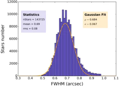
This is very consistent with our measured image quality. Fig-ure8shows maps of the median image quality per sub-tile image measured on unsaturated stars over the four CFHTLS fields. The number of stars used to determine the image quality was of the order of one hundred per sub-tile image. The histogram of the FWHM of all the stars used is represented in Fig.9.
We have explored the variation of the image quality over the WIRCam images. Figure10shows the x and y position of all unsaturated stars used for the photometric calibration (see Sect. 3.4). Despite the variations in seeing, one can note the spatial variations across the WIRCam field of view. The image quality is generally worse at the edge of the field. A region at the bottom left corner of the image shows very poor image quality, attributed to detector issues since this region is adjacent to a region of very poor cosmetics and dead pixels. This bad quality region has been subsequently masked in the CFHQSIR data.
3 Adjacent CFHTLS tiles overlap by a few arcminutes.
Fig. 8: Maps of image quality over the four CFHTLS fields. One square or rectangle of uniform colour corresponds to the foot-print of each WIRCam stack.
Fig. 9: Histogram of the image quality over the whole survey data.
4.2. Sensitivity
4.2.1. Correlated noise correction
Image resampling introduces correlations in the noise that should be accounted for in the photometric error budgets. Dis-cussions of this effect can be found for instance in Casertano et al. (2000), Labbé et al. (2003) (Sect. 4.4 and equation 3 therein),Grazian et al.(2006) andClément et al.(2012).
Noting ΦSE, the signal measured by SExtractor on an
aper-ture of Npixpixels, the photometric error measured by SExtractor
in the background dominated regime can be written as σΦSE = σpix×
p
Npix, (1)
where σpixis the local pixel to pixel standard deviation of the
background signal.
Article number, page 6 of 12
Fig. 8.Maps of image quality over the four CFHTLS fields. One square or rectangle of uniform colour corresponds to the footprint of each WIRCam stack.
A&A proofs: manuscript no. paper
stack. We require that a minimum of six zero points be measured in each stack. When there are less than six zero points, which happened for nine stacks only over a total of 1445), we assigned the average zeropoint of the corresponding CFHTLS field. For these nine stacks, this may represent an additional photometric error of less than 10%.
The illumination correction reduced the overall dispersion of the zero points from 10% to 7%, consistent with the amplitude of the illumination correction map. Finally, for consistency with the CFHTLS data (Hudelot et al. 2012), we normalize each stack by setting the zero point to a value of 30.0 in the AB system. 3.5. Registration to the CFHTLS format
For ease of use in connection with the CFHTLS data, we de-cided to produce one-square-degree image tiles similar to the CFHTLS data format, in addition to the WIRCam stacks. We use SCAMP (Bertin 2006) to determine the geometrical trans-formation between the reference z-band CFHTLS tile and the nine WIRCam stacks corresponding to this tile. In practice, the transformation is determined for each of the four quadrants of the WIRCam stacks using a three-degree polynomial. We then use SWarp (Bertin et al. 2002) to apply these transformations using a LANCZOS3 (Lanczos-3 6-tap filter) interpolation kernel and to reformat the whole dataset to the CFHTLS tile format.
When there is overlap between adjacent WIRCam stacks within a tile, all the pixels in the overlapping regions are used. Conversely, pixels in overlaps between tiles3 are treated
inde-pendently.
4. Main properties of the survey
We present in this section the main properties of the CFHQSIR survey data. We perform the analysis either on the WIRCam stacks or on the one-square-degree images mapped into the CFHTLS format (tiles) described in the previous section. We fur-ther divide each tile into 3 × 3 sub-images corresponding to the footprint of each WIRCam stack.
4.1. Image quality
All observations were carried out in service mode, with an IQ constraint in the K-band of 000.55 to 000.65, which translates,
as-suming a seeing limited image, to 000.65 to 000.75 in the Y-band.
This is very consistent with our measured image quality. Fig-ure8shows maps of the median image quality per sub-tile image measured on unsaturated stars over the four CFHTLS fields. The number of stars used to determine the image quality was of the order of one hundred per sub-tile image. The histogram of the FWHM of all the stars used is represented in Fig.9.
We have explored the variation of the image quality over the WIRCam images. Figure10shows the x and y position of all unsaturated stars used for the photometric calibration (see Sect. 3.4). Despite the variations in seeing, one can note the spatial variations across the WIRCam field of view. The image quality is generally worse at the edge of the field. A region at the bottom left corner of the image shows very poor image quality, attributed to detector issues since this region is adjacent to a region of very poor cosmetics and dead pixels. This bad quality region has been subsequently masked in the CFHQSIR data.
3 Adjacent CFHTLS tiles overlap by a few arcminutes.
Fig. 8: Maps of image quality over the four CFHTLS fields. One square or rectangle of uniform colour corresponds to the foot-print of each WIRCam stack.
Fig. 9: Histogram of the image quality over the whole survey data.
4.2. Sensitivity
4.2.1. Correlated noise correction
Image resampling introduces correlations in the noise that should be accounted for in the photometric error budgets. Dis-cussions of this effect can be found for instance in Casertano et al. (2000), Labbé et al. (2003) (Sect. 4.4 and equation 3 therein),Grazian et al.(2006) andClément et al.(2012).
Noting ΦSE, the signal measured by SExtractor on an
aper-ture of Npixpixels, the photometric error measured by SExtractor
in the background dominated regime can be written as σΦSE = σpix×
p
Npix, (1)
where σpixis the local pixel to pixel standard deviation of the
background signal.
Article number, page 6 of 12
Fig. 9.Histogram of the image quality over the whole survey data. Casertano et al.(2000),Labbé et al.(2003; Sect. 4.4 and Eq. (3) therein),Grazian et al.(2006), andClément et al.(2012).
Noting ΦSE, the signal measured by SExtractor on an
aper-ture of Npixpixels, the photometric error measured by SExtractor
in the background dominated regime can be written as σΦSE= σpix×
p
Npix, (1)
where σpix is the local pixel to pixel standard deviation of the
background signal.
To take into account the correlated noise, the photometric error will be multiplied by a corrective excess noise factor fcorr:
σΦ= fcorr× σΦSE = fcorr× σpix× p
Npix. (2)
To determine fcorr, we proceed as described inClément et al.
(2012) by measuring the variance of the flux measured in object-free apertures randomly positioned in an image:
1. For a given CFHQSIR tile, we select 2000 positions corresponding to source-free background regions. This is