Changes in aerosol properties during spring-summer period in the Arctic troposphere

(1)

HAL Id: hal-00302539

https://hal.archives-ouvertes.fr/hal-00302539

Submitted on 25 Jan 2007

HAL is a multi-disciplinary open access

archive for the deposit and dissemination of sci-entific research documents, whether they are pub-lished or not. The documents may come from teaching and research institutions in France or abroad, or from public or private research centers.

L’archive ouverte pluridisciplinaire HAL, est destinée au dépôt et à la diffusion de documents scientifiques de niveau recherche, publiés ou non, émanant des établissements d’enseignement et de recherche français ou étrangers, des laboratoires publics ou privés.

Changes in aerosol properties during spring-summer

period in the Arctic troposphere

A.-C. Engvall, R. Krejci, J. Ström, R. Treffeisen, R. Scheele, O. Hermansen, J.

Paatero

To cite this version:

A.-C. Engvall, R. Krejci, J. Ström, R. Treffeisen, R. Scheele, et al.. Changes in aerosol properties dur-ing sprdur-ing-summer period in the Arctic troposphere. Atmospheric Chemistry and Physics Discussions, European Geosciences Union, 2007, 7 (1), pp.1215-1260. �hal-00302539�

(2)

ACPD

7, 1215–1260, 2007

Spring summer aerosol in the Arctic

troposphere

A.-C. Engvall et al.

Title Page Abstract Introduction Conclusions References Tables Figures ◭ ◮ ◭ ◮ Back Close Full Screen / Esc

Printer-friendly Version Interactive Discussion

EGU

Atmos. Chem. Phys. Discuss., 7, 1215–1260, 2007 www.atmos-chem-phys-discuss.net/7/1215/2007/ © Author(s) 2007. This work is licensed

under a Creative Commons License.

Atmospheric Chemistry and Physics Discussions

Changes in aerosol properties during

spring-summer period in the Arctic

troposphere

A.-C. Engvall1, R. Krejci1, J. Str ¨om2, R. Treffeisen3, R. Scheele4, O. Hermansen5, and J. Paatero6

1

Department of Meteorology, Stockholm University, Stockholm, S 10691, Stockholm, Sweden

2

Department of Applied Environmental Science – Atmospheric Science Unit, University of Stockholm, Stockholm, S 106 91, Stockholm, Sweden

3

Alfred-Wegener-Institut f ¨ur Polar- und Meeresforschung, Telegrafenberg A43, D-14473 Potsdam, Germany

4

Koninklijk Nederlands Meteorologisch Instituut, Postbus201, NL 3730, AE De Bilt, Netherlands

5

Norsk institutt for luftforskning, Postboks100, 2027 Kjeller, Norway

6

Finnish Meteorological Institute, P.O.B. 503, FI-00101 Helsinki, Finland

Received: 13 November 2006 – Accepted: 19 December 2006 – Published: 25 January 2007 Correspondence to: A.-C. Engvall ([email protected])

(3)

ACPD

7, 1215–1260, 2007

troposphere

EGU Abstract

The change in aerosol properties during the transition from the more polluted spring to the clean summer Arctic troposphere was studied. A six year data set of obser-vations from Ny- ˚Alesund, Svalbard, covering the months April through June serve as the basis for the characterisation of this time period. In addition four-day-back trajec-5

tories were used to describe air mass histories. The observed transition in aerosol properties from an accumulation mode dominated to an Aitken mode dominated size distribution is discussed with respect to long-range transport and influences from natu-ral and anthropogenic sources of aerosols and pertinent trace gases. Our study shows that the air-mass transport is an important factor modulating the physical and chemical 10

properties observed. However, the air-mass transport cannot alone explain the yearly repeatable systematic and rather rapid change in aerosol properties, occurring within a limited time window of approximately 10 days. With a simplified phenomenological model, which delivers the nucleation potential for new particle formation, we suggest that the rapid shift in aerosol microphysical properties between the Arctic spring and 15

summer is mainly driven by the incoming solar radiation in concert with transport of precursor gases and changes in condensational sink.

1 Introduction

The Arctic environment has become a focus of the international scientific community during the last several decades due to its vulnerable ecosystem and climate system. 20

Recent studies on the Arctic climate showed that due to its sensitivity to external per-turbations, the Arctic could be seen as possible early warning of global climate change. Nowadays climate models predict the largest increase of the annual mean temperature for the Arctic (ACIA report, 2005).

Unlike for many other regions, there are only very few local human-derived sources 25

(4)

Arc-ACPD

7, 1215–1260, 2007

troposphere

EGU

tic. Therefore, transport of pollution including aerosols and its gaseous precursors from industrialized mid-latitude regions in Europe, Asia, and North America are of great im-portance. It is suspected that interactions between solar radiation, high surface albedo, the aerosol particles and clouds magnify the radiative impact of atmospheric aerosols (Quinn et al. 2002) in the Arctic region. Thus, for a given aerosol distribution the specific 5

optical impact is most likely increased in this high latitude region.

Previous experiments conducted over the last 40 years have mainly focused on the Arctic Haze phenomenon that occurs during late winter and spring. This was first noted in the literature by Mitchell (1957). Several years later scientist showed the seasonality of this phenomenon and that it was caused by anthropogenic sources at lower latitudes, 10

especially from the Eurasia continent (Rahn, 1981; Barrie, 1986; Heintzenberg, 1989). Further studies show that the chemical composition appears to have a very strong annual variation with higher loadings of anthropogenic components during late winter and early spring compared to the summer months (Heintzenberg and Larssen, 1983; Beine, 1998; Sirois and Barrie, 1999; Quinn et al. 2002).

15

Apart from the air chemistry, ground-based measurements from the Zeppelin station, Svalbard, and Point Barrow, USA showed that the aerosol loading undergoes a system-atic change from spring to summer (Quinn et al., 2001, Str ¨om et. al., 2003). Results from these studies demonstrated that there is an increase of aged particles, i.e. ac-cumulation mode particles larger than 100 nm diameter in winter and spring, which 20

are associated with anthropogenic sources and long range transport. In summer, this mode is significantly smaller in terms of number density. Smaller sized aerosols, so called Aitken mode particles, which range between about 20 and 100 nm, dominate the size distribution. At the same time the total number density increases.

In this study we will put emphasis on the transition from the more anthropogenic-25

influenced spring to clean summer conditions. It will be shown, that the transition from spring-type aerosol to summer-type aerosol occurs almost at the same time from year to year within a few weeks. We have selected different observational data in order to answer the question if this transition is mainly controlled by changes in the transport of

(5)

ACPD

7, 1215–1260, 2007

troposphere

EGU

pollutants or if this is an effect of local processes in the Arctic. Transport patterns, trace gases and aerosol microphysics are investigated for the period April through June for the years 2000–2005.

2 Air mass trajectories and long-term measurements from the Zeppelin station

2.1 Air mass trajectories 5

Using the model TRAJKS (Stohl et al., 2001) three-dimensional four-day back trajec-tories were provided by the Royal Netherlands Meteorological Institute (KNMI). These were used to study the link between air mass origin and the aerosol properties. The trajectories were calculated on daily basis at 12:00 UTC in a regular grid centred at

Ny-˚

Alesund (79◦_{N, 11.9}◦_{E) for period April through June during years 2000–2005. The}

10

grid contains beside the point of Ny- ˚Alesund four surrounding additional points in an al-most symmetric grid of more than 100 km sides. Two of the points are located over sea (78.5◦_{N 14.5}◦_{E) and (79.5}◦_{N 14.5}◦_{E) and the other two are located over land (78.5}◦_N

9.5◦_{E) and (79.5}◦_{N 9.5}◦_{E). The objective to investigate this grid was to demonstrate}

how representative the trajectories to Ny- ˚Alesund are for a larger area of interest and 15

to see possible difference between sea and land areas. Results from this study show that the flow pattern is essentially identical for all five chosen points. Thus for further calculations only the trajectories calculated for Ny- ˚Alesund (79◦_{N, 11.9}◦_{E) were used.}

In vertical, we investigate if there are any systematic differences in air transport be-tween the boundary layer (BL) and free troposphere (FT) over the investigated period. 20

The Micro Pulse Lidar (MPL) operated by the National Institute for Polar Research (NPIR) often show cloud tops around 2000 m altitude (Shiobara et. al., 2003). We thus define this altitude as the border between the BL and FT. The 1000 m and 5000 m alti-tudes are then taken to represent airflow in the BL and FT, respectively. Note that the Arctic atmosphere may present several stable layers and surface inversions are often 25

(6)

ACPD

7, 1215–1260, 2007

troposphere

EGU

“weather” (clouds and precipitation), which is why we use the altitude range indicated by the Lidar.

2.2 Long-term measurements

Aerosol particle number density, aerosol size distribution, SO₂, CO and210Pb obser-vations at the Zeppelin station

5

The long-term measurements at the Zeppelin station were used to evaluate tempo-ral variation of the spring-to-summer transition in aerosol properties on a multi-annual basis. The Zeppelin station is located on Mount Zeppelin 474 m above sea level in the community of Ny- ˚Alesund, Svalbard. Given the elevated location of the Zeppelin sta-tion the effect of local particle sources such as from the Ny- ˚Alesund community itself, 10

sea spray and resuspension of dust are strongly reduced. However, occasionally the sea salt and dust can contribute significantly to the total mass of the particles. Wind fields over Svalbard are complex due to the topography and surface characteristics. Compared to ocean level observation the effects of local wind phenomenon, such as katabatic winds are reduced at the Zeppelin station. Measurements of chemical and 15

physical properties at the Zeppelin station are included in the Cooperative Programme for Monitoring and Evaluation of the Long-range Transmission of Air Pollutants in Eu-rope (EMEP) and the Global Atmosphere Watch (GAW) programme coordinated by the World Meteorological Organization (http://www.wmo.int). Further information about the instrumentation and database are summarized at the homepagehttp://www.emep.int. 20

In this study we use aerosol data obtained at the station including number density, size distributions and activity of the radioactive component lead-210 (210Pb). In addi-tion we also use sulphur dioxide (SO₂) and carbon monoxide (CO) measurements to analyse the history and origin of the air masses. Table 1 gives an overview of data availability for the time period of 2000 through 2005 of all data from Zeppelin station 25

used in this study. In general the data availability is typically better than 90% each year, but some years are not covered by all variables. Year 2002 has low data coverage for aerosol microphysics and only less than 50% of210Pb data are available for year 2004.

(7)

ACPD

7, 1215–1260, 2007

troposphere

EGU

The physical properties of the aerosols such as the total particle number density and the size distribution are provided by the Department of Applied Environmental Science, Atmospheric science unit (ITM) at Stockholm University. Hourly data from the Zeppelin station includes total aerosol number density for particles larger than 10 nm (N₁₀) using a TSI 3010 Condensation Particle Counter (CPC) and size distribution that covers the 5

size range from 20 nm to 630 nm for year 2000 through 2005. The size distribution observations are carried out using a custom build Differential Mobility Particle Sizer (DMPS) based on a Hauke type Differential Mobility Analyzer (DMA) (Knutson and Whitby, 1975) coupled to a CPC model TSI 3010. This system uses a closed loop sheath air circulation described in Jokinen and M ¨akel ¨a (1997). The aerosol sample 10

flow is 1 L min−1_{, while the sheath airflow is set to 5.5 L min}−1_{. This yields a rather}

broad transfer function, but improves counting statistics during periods of low aerosol loading. When the total number concentration is ∼100 cm−3_{, the uncertainty arising}

from counting statistics, in the size classes close to mode of the size distribution is less than 5% (one standard deviation). The mobility distribution measured by the DMA is 15

inverted to a number distribution assuming a Fuchs charge distribution (Wiedensohler, 1988). The final data is given as hourly average. As the number concentration range over several orders of magnitude the means are calculated as geometric means.

No dedicated cloud-detecting device is available at the Zeppelin station. However, typically when the station is in cloud, it is represented by low accumulation mode parti-20

cle (diameter>0.1 µm) number density as the cloud drops scavenge aerosols from the

air. Aerosol characteristics during cloud events are very much affected by the cloud itself and we make a rudimentary data reduction in an attempt to reduce the impact of cloudy episodes. From our experience with the data set we choose an accumulation mode (90–530 nm) number density of 35 cm−3

as a threshold to indicate cloud-affected 25

aerosols. Hence, these data were removed from the data set, which corresponds to a data reduction of 22%.

The Norwegian Institute for Air Research (NILU) performs long-term measurements of sulfur dioxide (SO₂) and carbon monoxide (CO). Daily SO₂ gas concentrations are

(8)

ACPD

7, 1215–1260, 2007

troposphere

EGU

measured with KOH-impregnated Whatman 40 filter and further analysed with an ion chromatography. Gas chromatography with mercuric oxide reduction detection is used for CO measurements (Beine, 1998).

The Finnish Meteorological Institute (FMI) provides data of the activity concentration of lead-210 (210Pb) on aerosols. 210Pb concentrations are measured by collection 5

with a hi-volume aerosol particle sampler onto glass fibre filters (Munktell MGA). The sampler is made of stainless steel. The flow rate is ca. 120 m3h−1 _{and is measured}

with a pressure difference gauge over a throat. Three samples per week were collected with filter changes on Mondays, Wednesdays and Fridays. One out of 25 filters are left unexposed and is used as a field blank sample. The measurement of210Pb is carried 10

out by alpha counting of the in-grown polonium-210 (Mattsson et al., 1996; Paatero et al. (2003). We investigate data for five years 2001 to 2005 (see Table 1). Availability of data for each year is 100% except of 2004 when only 43% of data are available.

3 The spring to summer aerosol transition

3.1 Total number density 15

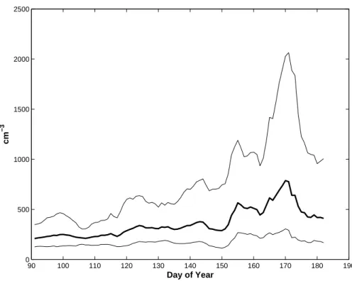
Due to a large range in the number densities, daily geometric means are calculated based on the hourly arithmetically averaged data. The temporal evolution of N₁₀ is presented in Fig. 1. To emphasis major trend in data, a running mean using a weekly window was applied.

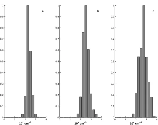
The changing pattern from month to month is evident from the frequency distribution 20

of N₁₀ number densities presented in Fig. 2. The months of April and May show a mode around 200 to 300 cm−3 _{and only few occasions when aerosol number density}

exceeds 1000 cm−3_{. June on the other hand shows a frequency distribution that is}

skewed towards higher aerosol number densities reaching several thousands per cubic centimetre.

(9)

ACPD

7, 1215–1260, 2007

troposphere

EGU

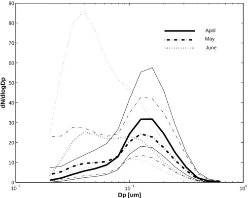
3.2 Particle size distribution

To illustrate major changes in aerosol size distribution we present a multi year compos-ite of monthly mean size distributions for each of the three months from April through June in Fig. 3. From Fig. 3 it is clear that a shift from an accumulation-dominated distribution to an Aitken-dominated size distribution occurs over the period from April 5

through June. The integral number density for the different distributions do not change dramatically and range from 200, through 250, to 300 cm−3_{for the consecutive months.}

When including smaller particles (N₁₀) the change in the integral number density from 203 cm−3 _{in April to 406 cm}−3 _{in June (see Table 2) is more pronounced. Hence,}

sim-ple approximation can be drawn, that around one quarter of the N₁₀ aerosol is smaller 10

than 20 nm in June.

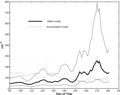
Based on the size range of the measurements and data availability we term particles between 22 and 90 nm Aitken mode particles and between 90 and 560 nm Accumu-lation mode particles. The temporal evolutions of these two modes are presented in Fig. 4 as weekly running geometric mean and standard deviation over the six years pe-15

riod. The Accumulation mode number density shows a general decrease over the time period. However, the trend is not so clear within the given data variability. In contrast, the Aitken mode number density show more structure in the way that an increase from around day of the year (DOY) 150 is evident in both mean and in variability indicating increasing importance of the periods with very high aerosol number densities.

20

Although primary aerosol sources such as sea spray exist in the Arctic, the Aitken mode particles are dominantly as a result of secondary particle formation. Through condensation and coagulation the newly formed particles grow into the Aitken mode. These processes will affect the growth of the particles and their residence time in a cer-tain size interval, hence coagulation and condensation are major sources of variability 25

for the Aitken mode particles (Williams et al., 2002).

In Fig. 4 the crossover between an accumulation-mode dominated to an Aitken dom-inated size distribution occurred around DOY 140 to 150, which corresponds to the last

(10)

ACPD

7, 1215–1260, 2007

troposphere

EGU

part of May.

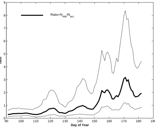
To explore this transition further we generated an alternative figure where we make use of the ratio between the two modes. In Fig. 5a running mean of the ratio

N_(22−90)/N_(90−560) from all available data between 2000–2005 is presented. Low

num-bers below one representing that accumulation mode particle dominates the size dis-5

tribution and vice versa for values above one. From Fig. 5 we see that the ratio around DOY 150 quickly exceeds and remains above 1.5. This indicates that once the change takes place the magnitude of the change in the distribution also increases.

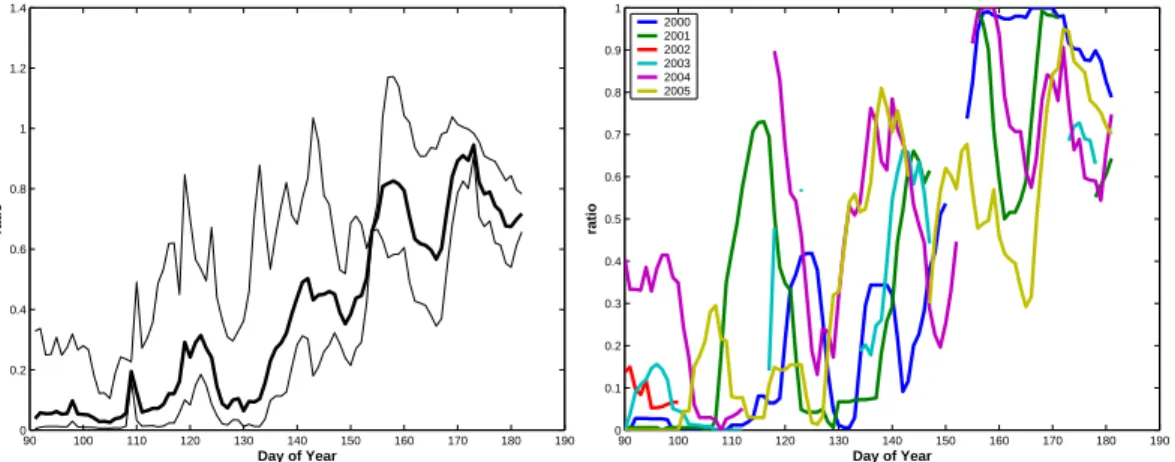
The change in shape of the aerosol size distribution can be also viewed in terms of persistence. In Figs. 6a–b the ratio of days for which the Aitken mode number 10

density is larger than the accumulation mode over a weekly window is presented. We term this the Aerosol Transition Index (ATI). The ATI appear to provide a more distinct measure of when the atmosphere has reached summer conditions i.e. dominance in Aitken mode particles. This can be defined at the point when the index reaching and remaining above 0.4 and last for at least 10 days. To study the year-to-year variability 15

we calculated this index for each year (Fig. 6b). We note that all six years have reached summer conditions based on this index by day 145 using the threshold defined above. All years are rather similar with respect to the temporal evolution and to when the final transition takes place and differ only within 5–10 days. Taking into account that a weekly window is used this implies that the transition from spring to summer is completed 20

within typically two weeks from year to year.

4 Coupling between aerosol properties, anthropogenic tracers and air mass transport and aerosol microphysics

4.1 Long-range transport

Eneroth et al. (2003) summarized the seasonal variation of the transport patterns to 25

(11)

pe-ACPD

7, 1215–1260, 2007

troposphere

EGU

riod 1991–2001. Five-day back-trajectories were calculated two times a day (00:00 and 12:00 UTC) and divided into eight major transport patterns (clusters). Their study showed the variability of the atmospheric circulation, in a synoptic scale, month-to-month and year-to-year. They derived clear seasonal differences due to the difference in the strength of pressure gradients between the seasons. Longest trajectories (equal 5

to a fast transport from lower latitudes of the Atlantic and Eurasia continent) are found during winter time and shortest (equal to a slow transport) during summer. Spring, defined as mid April to May, is associated with stable weather conditions and low cy-clonic activity. The stable weather conditions favour persistent airflow from the Arctic, and slow transport from northern part of Russia, Scandinavia and the Atlantic. The 10

fast transport associated with storm tracks from the Atlantic is shown to be infrequent during this period. Summer period i.e. June, July and August is associated with weak pressure gradients. During this period the transport from anthropogenic sources is not as efficient as in winter and spring.

In this section we will extend their study and emphasize on airflow patterns over 15

a limited period of the year and furthermore link air-mass transport, anthropogenic tracers and aerosol properties. Our aim is to produce an overview of the temporal evolution of the air transport to Ny- ˚Alesund.

4.1.1 Vectorized trajectories

For this study we have calculated 546 4-day-back trajectories for two altitude levels, 20

1000 and 5000 m, from April through June for the years 2000 through 2005 (see details Sect. 2). Handling of this large amount of trajectories requires synthesising the data into a more hand-able data that can be coupled to other tracer data. Therefore a variable called “trajectory vector” was derived. For each trajectory the radius of gyration was calculated. This summarises all the intermediate time steps of the trajectory into 25

one vector, with a direction and magnitude. The direction yields the main flow direction of the trajectory and the magnitude yields and indication on the speed with which the air travelled.

(12)

ACPD

7, 1215–1260, 2007

troposphere

EGU

From this trajectory vector we further are able to calculate the north-south (N-S) and east-west (E-W) contribution of the air-mass transport to Ny- ˚Alesund. These open up the possibility to reduce the air mass trajectory information into single parameter and produce time series, which allow investigation of the air mass transport temporal evolution. Further we use these trajectory vector time series to evaluate the hypothesis 5

that the air-mass transport controls the transition of the aerosol properties between spring and summer.

The coordinates are relative to Ny- ˚Alesund 79◦_{N 11.9}◦_{E i.e. projection of the}

trajec-tory vector to the x-axis give us the contribution in the E-W direction relative to longitude 11.9◦ _{and projection to the y-axis the contribution in the N-S direction of latitude 79}◦_N.

10

A positive (negative) value of the x- and y-axis represents air from the east (west) and north (south).

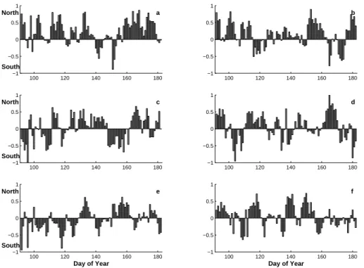
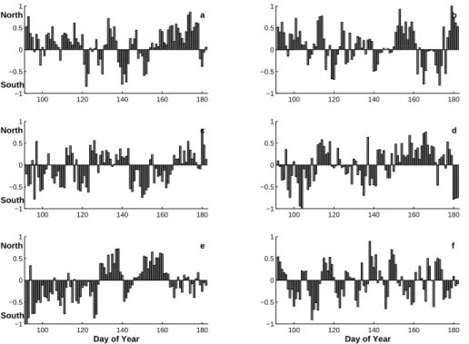
4.1.2 Transport patterns

Combining the N-S and E-W components for each day gives us the horizontal informa-tion of the trajectory with respect to the direcinforma-tion and magnitude. Fig. 7a–b presents 15

the calculated N-S contribution for each day trajectory arriving to level 1000 m (BL) and 5000 m (FT) for the time period from 2000 through 2005.

Comparing the different years for the fraction of the N-component an about a fifty-fifty contribution of the different wind components. The fraction of the N-component for each year (2000 through 2005) at level 1000 m (5000 m) is 66(65)%, 61(56)%, 49(44)%, 20

51(48)%, 41(40)%, and 55(43)% (cf. Fig.s 7a-b). To give some value how well the vectors between the two levels follow each other the correlation coefficients for the N- S-contribution have been calculated. For each year the result is R₂₀₀₀=0.75, R2001=0.73,

R₂₀₀₂_{=0.62, R}₂₀₀₃_{=0.64, R}₂₀₀₄_{=0.70, R}₂₀₀₅_{=0.63. The rather low correlation indicates} differences in the wind patterns at the two altitudes. From Fig. 7 there are no apparent 25

trends that could link to and explain the transition in aerosol properties.

The analysis above has essentially provided information about the horizontal trans-port. To investigate the vertical dimension we also calculated the time the trajectory

(13)

ACPD

7, 1215–1260, 2007

troposphere

EGU

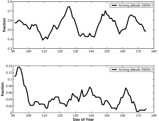
has spent in the boundary layer during the last 4 days of its transport to Ny- ˚Alesund. The different years are then averaged for each day of the investigated time period and are expressed as fraction time to the total time-length of the trajectory. In this context we define generally altitudes below 2000 m as BL. This altitude often represents the top of the low level clouds as seen by micro pulse lidar at Ny- ˚Alesund. The excep-5

tions are cases when the air arrives within a sector that belongs to the Arctic basin i.e. representing the area within the two tangents that origins in the coordinates of

Ny-˚

Alesund and tangents the north coast of Greenland and the northern coast of Siberia. Within this sector the BL height is defined as 1000 m. This difference in definition in BL is taking into account the stable stratification over the pack ice, especially during the 10

summer months (Nilsson et al., 1999).

The calculated fraction ranges from 0 to 1, where 1 represents a trajectory spends all its time in the BL. The temporal evolution of this fraction is depicted in Fig. 8. The upper panel of Fig. 8 represents trajectories arriving to Ny- ˚Alesund at the altitude level 1000 m and the lower panel trajectories arriving to altitude level of 5000 m. Not surprisingly 15

trajectories arriving at a lower altitude spend more time in the BL. Comparing the start and end of the period, we notice a decreasing trend in ratio of high-level trajectories spending its time in the BL (bottom Fig. 8). But these trends are not very strong and do not show the radical change between DOY 140 and 150 as the aerosol properties do. 4.2 Anthropogenic tracers

20

In previous section we have shown that transport alone does not explain the transition in aerosol properties observed on annual basis. Here we will explore possibility that the combination of various transport patterns and seasonal changes in the anthropogenic sources strength can shed a light on observed aerosol microphysics. To follow this hy-pothesis we used data of anthropogenic tracers namely SO₂, CO and210Pb observed 25

at the Zeppelin station and focused on their temporal variation. SO₂is one of the major anthropogenic trace gases and highly relevant to aerosol properties. However, it also has a natural biogenic source contributing to SO₂in the atmosphere through oxidation

(14)

ACPD

7, 1215–1260, 2007

troposphere

EGU

of DMS (Li and Barrie 1993, Li et al. 1993). Therefore, we also explored measure-ments of CO and210Pb because in the Arctic the occurrence of these can be attributed exclusively to anthropogenic activities and continental regions, and we will use them as major tracers for anthropogenic source regions (Beine, 1998; Paatero, 2003).

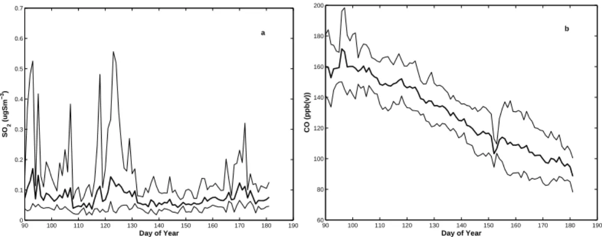
Figure 9a and b shows the weekly running mean of SO₂ and CO. SO₂ shows a 5

large inter-annual variability in data for the period April through June with episodes of high values in April and May and rather low concentration in June. Sulphur diox-ide concentrations range between a minimum value of 0.01µgSm−3 _(effective

detec-tion limit) to a maximum value of 2.13µgSm−3 _{and a median of 0.07}_µgSm−3_{. The}

monthly mean and standard deviation of SO₂ show their maximum to occur in May 10

with 0.14(0.28)µgSm−3 _{and a trend that decreases towards June with corresponding}

values of 0.07(0.04)µgSm−3_{(cf. Table 2).}

The high variability of SO₂ in April and May reflects the frequent fast transport from anthropogenic sources that take place during springtime whereas the June is more as-sociated with lower background concentrations perturbed by occasional higher values 15

but not as high as April and May. For year 2005, SO₂ show a mean concentration of 0.13µgSm−3

, which differ from other years where the mean concentration is much lower (0.07µgSm−3_{). Over all years we note that after day 140 SO}

2 infrequently

ex-ceeds 0.07µgSm−3_{. The only characteristic that could relate to the aerosol transition}

is the fewer occurrences of higher SO₂levels after DOY 140. However, this trend would 20

tend to decrease the potential for new particle formation.

CO in Fig. 9 follows a clear decreasing trend from April through June. Carbon monox-ide has a longer lifetime in the atmosphere than SO₂, about 90 days compared to about a week, which explains much of different features presented in Fig. 9. The total mean and standard deviation for all included years from 2002 to 2004 of CO concentration is 25

135(25) ppbv which is about 9% lower compared to yearly based mean of 146.7 ppbv (Beine, 1998). Beside some small deviation around DOY 155, the trend in mean values shows no special features and rather smoothly decreases with time. Variability is also rather constant over the time period.

(15)

ACPD

7, 1215–1260, 2007

troposphere

EGU

The annual cycle of hydroxyl radical (OH) is of major importance for the seasonal evolution of CO as OH acts as a major sink for CO. OH is produced by photochemical reactions and therefore depends on the incoming solar radiation. Observations show that the CO accumulates in the Arctic troposphere during wintertime due to transport processes and the fact that sink processes by OH are not available (Dianov-Klokoc 5

and Yarganov, 1989). During spring when the sun raises the sink processes for CO get active and the CO concentrations start to decrease and its minimum is reached in summer (Dianov-Klokoc and Yarganov 1989). The steady state decrease of CO mixing ratios only slightly perturbed by local maxima correlated with higher SO₂also indicates that dilution and mixing with clean air masses and photochemical sink of CO dominates 10

over the source in a form of long range transport during April–June period.

Lead-210 (210Pb) originates almost exclusively from continents and as such it is tracer of air masses having rather recent contact with landmasses. With its long life-time210Pb (half-life 22 years) the atmospheric lifetime is mainly governed by the lifetime of aerosols (Paatero et al. 2003). Most of the atmospheric210Pb is attached to accu-15

mulation mode aerosols. Based on the activity ratio of210Pb and its progeny; mean aerosol residence times can be estimated. Within this study we only look at the tempo-ral variation of210Pb data itself. Paatero et al. (2003) presented the annual variation of the activity concentration of210Pb at the Zeppelin station between 11 and 620µBqm−3

for the year 2001. The maximum was observed in March–April and the minimum in 20

summer. We calculated210Pb activity concentration between 0 and 552µBqm−3_{. The}

data presented in Fig. 10 agree well with Paatero et al. (2003) and his single year study, maximum values in April with a monthly mean and standard deviation of 165 and 134µBqm−3_{, respectively and a much lower mean in June, 35(27)}_µBqm−3_.

Lead-210 is one of the tracers investigated in this study that shows a more pro-25

nounced change around DOY 140. Together with a decrease in the mean activity, the variability also drops notably. It is worthy to note again that210Pb is associated with ac-cumulation mode particles and thus could be a proxy of relative increase or decrease of the aerosol surface area, which also are dominated by accumulation mode aerosol

(16)

ACPD

7, 1215–1260, 2007

troposphere

EGU

(Fig. 10b).

4.3 Coupling between the aerosols, anthropogenic tracers and air-mass transport In Sect. 3.2 we have demonstrated that the Aitken mode particles show an increas-ing trend in number density from April to June and the accumulation mode particles show a slow decreasing trend. With the obtained vectorized trajectories (see Sect. 4.1) 5

we will in this section couple the horizontal air-mass transport to the loading of the aerosols and the anthropogenic tracers loading for each day. Investigations have been performed for all years but we select one year, 2001, to illustrate our findings. For this year we have the most complete data set available (cf. Table 1).

Figure 11a (upper panel) shows the N-S component together with the daily average 10

of the accumulation mode (solid line) and Aitken mode particles (dashed line) and the lower panel the corresponding E-W component. Combining the information of these two plots one can follow the aerosol loading and the main direction of the air-mass transport.

Peak of accumulation mode particles reach values around 300 cm−3_{, which}

corre-15

sponds to the upper level of the variation of the number density (Fig. 4). The vectorized trajectories for these days, 125 and 132 (May), 165 and 172 (June), are characterised by north-east and south-east contributions.

The high accumulation mode number densities in May are connected to air masses arriving to Ny- ˚Alesund from northeast. A further look on the trajectories shows the 20

air mass origin from the northerly part of Russia and Siberia and they are most likely affected by pollution sources, e.g. metal smelter at Norilsk (Virkkula et al., 1995). The occasions in June show southeasterly air-transport and the air masses can be traced to Scandinavia and further south. Aiken mode particles show high number densities when the air masses originate in the north-west or south-west i.e. in the clean regions 25

of the Arctic basin and the Atlantic Ocean

Additional insight into the origin and sources of the high accumulation mode aerosol episodes can be done with help of SO₂ and 210Pb (Fig. 11b). SO₂ show two

(17)

spe-ACPD

7, 1215–1260, 2007

troposphere

EGU

cific peaks around day 125 and 130 in May, same as the accumulation mode aerosol (Fig. 11a) supporting the continental origin of the air mass and influence of the anthro-pogenic sources.

210

Pb data has a lower data rate (one sample about every third day) compared to particle data and SO₂data (reason for the non-continues line in Fig. 11c). This makes 5

it hard to make accuracy comparisons of210Pb and for individual values of accumula-tion mode densities and SO₂. As it is shown in Fig. 10a the averaged concentration of210Pb decrease during the period with an order of more than 5 from April through June. Why we also find the highest peak in April, day 95, which can be coupled to a weak northwesterly air-transport to Ny- ˚Alesund. The concentrations reach a value of 10

∼450 µBqm−3 compared to the median value of 133µBqm−3 for the specific period of this year 2001. This high value cannot be associated to any transport from continen-tal origin or to be coupled to any corresponding high values for SO₂ or accumulation mode particles. Further investigation of the trajectories shows that the air descending towards Ny- ˚Alesund originates from the American continent. In an earlier study the 15

effect of the North American continent on the airborne210Pb in northern Finland was observed (Paatero and Hatakka, 2000). As mentioned before the residence time for

210

Pb can vary from a few days up to a month depending on how effective the scaveng-ing of the particles from the atmosphere are. Less efficient scavengscaveng-ing of the particles might be the case of this observed max value. However, enhanced values later during 20

the period days 130–135 are within same period for when enhanced values of the den-sity of accumulation mode particles (Fig. 11a) and SO₂ (Fig. 11c) and are coupled to northeasterly flow from northern part of Eurasia.

The data presented show that the air mass origin and transport are important fac-tors controlling the aerosol microphysical properties, but against the expectations air 25

mass transport alone cannot explain at all the spring – summer transition in aerosol properties. Moreover, it is very likely that other processes are of the same or higher importance and this alternative scenario will be discussed in the following section.

(18)

ACPD

7, 1215–1260, 2007

troposphere

EGU

210_{Pb. On the other hand the lifetime of}210_{Pb in the atmosphere is intimately linked to}

aerosols through being attached to accumulation mode particles (see Fig. 10b). The accumulation mode particles are typically where the largest surface area can be found and thus is the largest sink for condensable species. New particle formation is a non-linear process that involves the competition between the sink of condensable species 5

and the source of the same. Therefore the alternative scenario can be formulated: Can annual systematic changes in the source strength and sink rate of the condensable species together give the type of transition that the aerosol properties show?

4.4 Nucleation potential 4.5 Method

10

To explore possible link between the observed spring-summer transition in aerosol size distribution with respect to aerosol nucleation potential we first assume that the new particle formation involves sulphuric acid (H₂SO₄). The equilibrium vapour concentra-tion of sulphuric acid is calculated for each day based on daily average data, for which the source rate and sink rate of H₂SO₄ is balanced. Following Kulmala et al. (2004) 15

the time dependent vapour concentration of H₂SO₄,C, can be written as d C

d t = Q − CS · C, (1)

whereQ is the source rate and CS the condensational sink. Equilibrium vapour

con-centration here refers to zero rate of change and is equal to _{d C/d t = 0 and thus a} balance of the source and sink. The equilibrium vapour concentration of H₂SO₄,C, is

20

then given by

C = Q

(19)

ACPD

7, 1215–1260, 2007

troposphere

EGU

4.5.1 Source

The source rateQ, is calculated by

k · OH · SO2, (3)

wherek is the reaction rate 10−12_(s−1_{) (Seinfeld and Pandis, 1998), and OH and SO} 2

are observed daily averages expressed as molecules per cm−3_{. The OH radical is}

5

not observed and was parameterized from the global radiation observationsS (Wm−2₎

(http://www.awi-bremerhaven.de/MET/NyAlesund/fulltimeresquery.html). To calculate OH concentration,S was simply scaled by a maximum value (387) of the total data set

for observed diffuse solar radiation and multiplied by 5·106according to Eq. (4).

S · 5 · 106

387 . (4)

10

As actual OH radical concentrations are unknown to us this scaling is entirely arbitrary and only serves to reproduce typical values for OH concentrations frequently reported in the literature (Seinfeld and Pandis, 1998).

4.5.2 Sink

The condensational sink (CS) is calculated based on observed size distributions fol-15

lowing Kulmala (2001), including the correction factor for the transition between the molecular and continuum regimes given by:

CS = 2πD ∞ Z 0 d_pβ_M(d_p)n(d_p)d d_p= 2πDX i β_Md_p,iN_i (5)

where_{D is the diffusion coefficient, n(dp) is the particle size distribution function and}

N_i is the concentration of particles in the size sectioni. For the transitional correction

(20)

ACPD

7, 1215–1260, 2007

troposphere

EGU

factor for the mass fluxβM we use the Fuchs-Sutugin expression (Fuchs and Sutugin, 1971).

To derive the condensational sink, CS (s−1_{), the hourly averaged size distributions}

for particles larger than 90 nm (accumulation mode particles) were used. The reason for restricting the condensational sink only to the accumulation mode particles is that 5

Aitken particles are a result of relatively recent particle production, whereas the accu-mulation mode particles most likely were already present and available as a sink at the time the new particles were formed.

CS was calculated from the hourly average of particle data. We exclude days with less than 10 data points (hourly averages). It should also be noted that CS is calculated 10

based on dry aerosol due to the measurement setup (see Sect. 2.2). Increase in particles’ size due to ambient relative humidity is not considered. Typically, the Arctic summer boundary layer is often very humid. In situations when humidity exceeds 80% the CS may be underestimated by a factor of 2–3, therefore our values of CS are very likely to be on the lower end of the possible range.

15

4.5.3 Result

Following the above formulas the equilibrium H₂SO₄ concentration was calculated based on the average incoming radiation, SO₂and condensational sink for each day. In Fig. 12 these values for the data set are plotted as function of day. The data ranges from close to zero to around 1·108molecules cm−3 _{with an increasing trend with time.}

20

We are interested to find out whether there is any particular value of C above which small particles are more likely to occur. To do this we analysed the observed integral aerosol number densities of various sizes versus C (Fig. 13a–c). There are different amount of data in each scatter plot presented in Figs. 13a–c due to data reduction of time resolution of the individual instruments. Note that data in 13a and 13b are entirely 25

independent, whereas in Fig. 13c the accumulation mode part of the size distribution enters both variables.

(21)

ACPD

7, 1215–1260, 2007

troposphere

EGU

densities as C increases. However, it is difficult to distinguish a very clear critical value for C that would indicate a nucleation threshold. Based on the three scatter plots it appears that a value of C above approximately 3·106 molecules cm−3 _{separates C}

values with generally low number densities and C values associated with the highest number densities.

5

Note that we work with daily averages given by measured data from Ny- ˚Alesund. The time that new formed particles need to reach a size of 10 nm (detectable size for the instrument) may take several hours up to a day due to the low concentration of condensable material in the Arctic. Hence, the observed conditions when there are high number densities of aerosols in Ny- ˚Alesund are not necessarily identical to the 10

conditions existing where the particle formation actually took place. To give the reader a feeling of the spatial scale of our approach we may think of how far an air parcel is transported in one day. Given a mean wind speed of 5 m s−1_{this distance is equivalent}

to more than 400 km transport during one day. This means that processes taking place 400 km from Ny- ˚Alesund affect our daily averages.

15

4.5.4 Trace gases influence on observed aerosol loading

Whether or not the critical value is below or above 3·106 molecules cm−3 _{we can see}

the potential effect of such threshold on the size distribution over time. We may think of it as a nucleation potential. Moreover, it is not only of interest if the conditions reach the threshold, but also to what extent C may exceed above these values, as seen from 20

Figs. 13a–c. We illustrate this by making weekly moving average of the ratio between the number of data points exceeding a certain threshold divided by the total number of data points for the time window over all six years. If the equilibrium threshold is reached often we expect that formation of particles occur readily during that time. The higher the value of this threshold is set the more vigorous we expect the particle formation to 25

be.

We explore three different values of H2SO4 equilibrium concentration threshold

(22)

differ-ACPD

7, 1215–1260, 2007

troposphere

EGU

ent ratios it is clear that changing the threshold from 0.6·107to 1.1·107molecules cm−3

have the largest impact on the evolution of the ratios in the middle of the time period where the reduction in the ratio is twice as large as in both end of the time period. Thus, the difference between the ratios in April and May compared with June are accentu-ated. This is most evident for the highest threshold value, where the ratio increases 5

from low values to about 0.2 over the first two months and then quickly increases to above 0.4 in about a week’s time.

A small amount of data (about 6%) is clearly affected by rapid transport from an-thropogenic sources evident in the very high SO₂ concentrations for the time period. These high SO₂concentrations would yield to enhanced values of equilibrium H₂SO₄. 10

As we only consider the aerosol size distribution up to 530 nm (due to the limitation of the measuring equipment) in calculating CS, it is possible that a significant contribu-tion to CS from larger particles is missed during strong pollucontribu-tion events. This would result in an underestimation of C, whereas nucleation events are typically quenched in polluted air due to large aerosol surface area. To test the influence of these events on 15

our results we repeated the ratio calculation after screening data where SO₂ exceed 0.6·107 molecules per cm−3 _{(Fig. 14b). This limit was chosen by investigating data}

for when SO₂concentration reached high values that probably were influenced by an-thropogenic sources. Excluding the pollution events makes no large changes between Figs. 14a and 14b. But excluding these outliers makes the transition from low ratios 20

in the beginning of the period to higher ratios in June somewhat clearer. The high-est threshold for instance never occurs before DOY 115. Between DOY 115 and DOY 145 the fraction of time the threshold is exceeded increases to 20%. Only 10 days later this fraction is more than doubled and from about DOY 155 the fraction wiggles around 50%. Hence in late May and beginning of June the occurrence of the potential 25

(23)

ACPD

7, 1215–1260, 2007

troposphere

EGU

5 Discussion

Transport patterns and source strengths of anthropogenic tracers change over the year with the net effect that the Arctic atmosphere in late winter and springtime is the most polluted period and the summer is the cleanest period of the year. Over this time period the aerosol change from being an accumulation mode dominated aerosol to become 5

an Aitken mode dominated aerosol. Our observations and analysis show that this transition is not typically a gradual change but occurs over a rather short time period each year.

Intrigued by the temporal persistence of the transition we investigated systematically pertinent tracers and transport patterns over the period April, May and June. Although 10

seasonal changes in the flow pattern exist (Eneroth et al., 2003; Stohl, 2006) our anal-ysis could not reveal any systematic pattern that could help explain the rapid transition observed for the aerosol properties.

The fact that the SO₂ values are at the lowest during the period with most active particle production is perhaps unexpected. Shaw (1989) discussed particle formation 15

in clean areas and suggested that one viable path way is the cleaning of pre-existing aerosol area through precipitating clouds. The temporal evolution of the condensational sink, CS, depicted as a weekly running mean in Fig. 15a indeed shows persistently low values from about DOY 150 and onwards. The temporal characteristics of CS in many ways resemble those presented by210Pb in Fig. 10a. As a matter of fact, the 20

correlation between these two variables is better than 0.92. As the210Pb is associated with accumulation mode particles this close relation can be understood.

At the same time as clouds remove pre-existing aerosol surface area and pave way for new particle nucleation, clouds also scavenge SO₂ through liquid oxidation and produce particulate sulphate on already existing particles. This removal of SO₂ will in 25

turn reduce the potential for subsequent nucleation of new particles. The fact that the monthly mean SO₂concentration is about half in June of what it is in April and May (c.f Table 2) is consistent with scavenging by the extensive clouds that occupy the Arctic in

(24)

ACPD

7, 1215–1260, 2007

troposphere

EGU

the summer period.

We note that whereas210Pb continues to decrease through out our period of inves-tigation, CS appears to recover at the end. As 210Pb is a tracer for continental air masses, this deviation between the two variables would be consistent with a rebuilding of the aerosol surface area that takes place within the Arctic basin or over ocean further 5

south. Given the typically low wind speeds in the Arctic summer atmosphere (Stohl, 2006; Eneroth et al., 2003; Heintzenberg, 1991), this decrease in210Pb and increase in CS is most likely the origin from secondary aerosol formation taking place within the Arctic.

A complicating aspect with respect to the discussion above about scavenging of SO₂ 10

by clouds is that, if one studies the temporal evolution of SO₂ over the last part of the time period it appears as if SO₂ increases (Fig. 9a). It is not obvious how to fit this behaviour with the observation of210Pb and CS above. On one hand it may be indica-tive of an increasing marine source of SO₂associated with the summer-time biological activity in the ocean through oxidation of dimethyl sulphide (DMS) and subsequent 15

formation to SO₂. On the other hand this increase may be a greater influence from an-thropogenic sources during parts of the summer as reported by (Heinzenberg, 1989). In the later case the scavenging of accumulation mode particles must be efficient while letting some fraction of SO₂survive the cloud passage or passages. Nevertheless, the question about the origin of SO₂in the summer Arctic, anthropogenic versus natural is 20

an interesting subject and related to aerosol-cloud interactions and climate forcing and needs further investigations.

The third leg in this simple method to determine the nucleation potential is solar radi-ation, which in turn is a proxy for OH in the atmosphere. Str ¨om et al. (2003) presented data that showed a close relation between the yearly cycle of particle number density 25

and incoming solar radiation at Ny- ˚Alesund, which supports the importance of photo-chemical reactions. At about mid-March the Sun returns to the Svalbard region and the summer solstice occurs about three weeks into June. Hence, the spring to summer pe-riod presents a dramatic increase in the amount of radiation that reaches Ny- ˚Alesund.

(25)

ACPD

7, 1215–1260, 2007

troposphere

EGU

Therefore, the decrease in the precursor gas SO₂due to changes in transport patterns is more than compensated by the combined effect of an increased radiation flux and a decreased condensational sink.

This is illustrated by using some simple numbers. Sulphur dioxide decreases by about a factor of two between the beginning and end of the time period (c.f. Table 2). 5

The condensational sink decreases over the same time by about a factor of 2 to 3 (cf. Fig. 15). However, the weekly median radiation increases by about a factor of 5 (Fig. 15b). Hence, the temporal evolution of CS and SO₂ largely compensate each other and the nucleation potential is mainly driven by the radiation. The net effect is that the nucleation potential is driven by planetary motions and will therefore reach 10

some critical value at about the same time each year.

Particle nucleation is highly non-linear and some critical super-saturation of con-densable vapours must be reached before new particles will form. Below this value nucleation does not readily occur. The more this critical value is exceeded the larger the chance is that the newly formed particles will grow to sizes that can be detected by 15

the instruments at the Zeppelin station for instance.

Based on the temporal evolution of the Aitken mode (Fig. 4) and the aerosol transition index (Fig. 6a and b) we believe that this critical value is typically met every year around DOY 145 plus minus a week. Hence we believe that photochemical reactions govern much of the aerosol dynamics in the Arctic.

20

6 Summary

The main motivation for this paper was to have a closer look on the spring – summer period (April, May and June), with emphasis on the transition in aerosol properties observed in the Arctic troposphere on annual basis. In the study we have used four-day-back trajectories and long-term observations of the aerosols and trace gases from 25

the Zeppelin station at Ny- ˚Alesund, Svalbard. We have described the differences be-tween periods, spring and summer, the transition bebe-tween them and we tried to link the

(26)

ACPD

7, 1215–1260, 2007

troposphere

EGU

observations to the large-scale circulation and to influences from natural and anthro-pogenic sources of aerosols and gases.

We have investigated the hypothesis that the air transport to the Arctic is control-ling the systematic change in the physical aerosol properties that are observed at the Zeppelin station. To summarise this work, we ended up with four main conclusions: 5

1. Using air mass back trajectories we have shown that the transport alone can-not explain the repeating transition from spring-type to summer-type in aerosol observed in the Arctic troposphere.

2. Blocking the advection of the polluted air masses from south into the Arctic is important contribution of the transport, but it should be seen more like a necessary 10

prerequisite instead of the main process controlling the spring-summer transition in aerosol properties

3. With a simplified model, which delivers the nucleation potential for new particle formation in a form of vapour equilibrium concentration of H₂SO₄we suggest that the aerosol microphysical properties are a result of a delicate balance between 15

incoming solar radiation, transport and condensational sink processes.

4. The temporal evolution of the condensational sink and SO₂ concentrations indi-cate that at large degree they compensate each other and the nucleation potential is mainly driven by the solar radiation. The net effect is that the nucleation poten-tial is driven by planetary motions and will therefore reach some critical value 20

about the same time each year. This is consistent with a repeating pattern of the aerosol transition between spring and summer.

The whole picture is further complicated by the fact that remote sensing data (Treffeisen et al., 2006) show the whole troposphere to be involved in a similar transition. Remote sensing within the Stratospheric Aerosol and Gas Experiment SAGE II and SAGE III 25

(27)

ACPD

7, 1215–1260, 2007

troposphere

EGU

aerosol in the upper free troposphere above approximately 4 km altitude (Treffeisen et al., 2006). At this time it is not clear how and to what extent these processes in the boundary layer and free troposphere are interlinked. In order to get better insight into this phenomenon, airborne in-situ measurements covering the whole tropospheric column are necessary.

5

Acknowledgements. The authors would like to acknowledge C. Lunder (NILU), B. Noone (ITM) and J. Weaher (ITM) for providing us with data from the Zeppelin station. The monitoring at the Zeppelin station is supported by the Swedish Environmental Protection Agency and by the Swedish national science foundation. Support is also received from the Swedish Polar Secretariat. The FMI’s210Pb measurements at Mt. Zeppelin are made in collaboration with the

10

Norwegian Institute for Air Research (NILU) and the Norwegian Polar Institute (NPI).

References

Barrie, L. A.: Arctic air pollution: an overview of current knowledge, Atmos. Environ., vol. 20, 643–663, 1986.

Beine, H. J.: Measurements of CO in the high Arctic, Global change science 1, 1999, 145–151,

15

1998.

Bodhaine, B. A. and Dutton, E. G.: A long-term decrease in Arctic-Haze at Barrow,Alaska, Geophys. Res. Lett., 20, 947–950, 1993.

Dianov-Klokov, V. I. and Yurganov, L. N.: Spectroscopic Measurements of Atmospheric Carbon Monoxide and Methane. 2: Seasonal Variations and Long-Term Trends, J. Atm. Chem. 8,

20

153–164, 1989.

Eneroth, K., Kjellstr ¨om, E., and Holm ´en, K. : A trajectory climatology for Svalbard; investigating how atmospheric flow patterns infuence observed tracer concentration, Phys. Chem. Earth, 28, 1191–1203, 2003.

Fuchs, N. A. and Sutugin, A. G.: Highly dispersed aerosols, Ann. Arbor Science Publ., Ann

25

Arbor, Michigan, 1970.

Heintzenberg, J. and Larsson, S.: SO2and SO4in the Arctic: interpretation of observations at

three Norwegian arctic-subarctic stations, Tellus, 35B, 255–265, 1983.

(28)

ACPD

7, 1215–1260, 2007

troposphere

EGU Heintzenberg, J., Str ¨om, J., Ogren, J.-A., and Fimpel, H.-P.: Vertical profiles of aerosol

prop-erties in the summer troposphere of the European Arctic. Atmos. Environ., 25A, 621–628, 1991.

Jokinen, V. and M ¨akel ¨a, J. M.: Closed-loop arrangement with criticalorifice fro DMA sheat/excess flow system, J. Aerosol Sci. 28, 643–648, 1997.

5

Knutson, E. O. and Whitby, K. T.: Aerosol classification by electric mobility: apparatus, theory and applicatons, J. Aerosol Sci., 6, 443–451, 1975.

Kulmala, M., Pet äj ä, T., M önkk önen, P., Koponen, I. K., Dal Maso, M., Aalto, P. P., Lehtinen, K. E. J., and Kerminen, V.-M.: On the growth of nucleation mode particles: source rates of condesable vapor in polluted and clean environments, Atmos. Chem. Phys., 5, 409–416,

10

2005,

http://www.atmos-chem-phys.net/5/409/2005/.

Kulmala, M., Dal Maso, J., M äkel ä, L., Pirjola, M., V äkev ä, P, Aalto, P., Miikkulainen, K., H ämeri, K., and O’dowd, C., D.: On the formation, growth and composition of nucleaton mode parti-cles, Tellus, 53B, 479–490, 2001.

15

Li, S.-M. and Barrie, L. A.,: Biogenic Sulfur Aerosol in the Arctic Troposphere: 1. Contributions to total sulfate, J. Geophys. Res., 98, No D11 20 613–20 622, 1993.

Li, S.-M., Barrie, L. A., and Sirois, A.,: Biogenic Sulfur Aerosol in the Arctic Troposphere: 2. Trends and seasonal variations, J. Geophys. Res., 98, No D11 20 623–20 631, 1993. Mattsson, R., Paatero, J., and Hatakka, J.: Automatic Alpha/Beta Analyser for Air Filter

Sam-20

ples – Absolute Determination of Radon Progeny by Pseudo-coincidence Techniques, Radi-ation Protection Dosimetry, 63(2), 133–139, 1996.

Mitchell, J. M.: Viusal range in the polar regions with particular referenceto Alaskann Arctic, J. Atmos. Terr. Phys. Spec. Suppl., 1995–211, 1957.

Paatero, J. and Hatakka, J.: Source Areas of Airborne7Be and 210Pb Measured in Northern

25

Finland, Health Physics, 79(6), 691–696, 2000.

Paatero, J., Hatakka, J., Holm ´en, K., Eneroth, K., and Viisanen, Y.: Lead-210 concentration in the air at Mt. Zeppelin, Ny- ˚Alesund, Svalbard, Phys. Chem. Earth, 28, 1175–1180, 2003. Seinfeld J. H. and Pandis, S. P.: Atmospheric Chemistry and Physics, A Wiley-Interscience

publication, 250, Canada, 1998.

30

Shaw, G. E.: Production of condensation nuclei in clean air by nucleation of H2SO4, Atmos.

Environ., 12, 2841–2846, 1989.

(29)

ACPD

7, 1215–1260, 2007

troposphere

EGU Lidar measurements at Ny- ˚Alesund, Svalbard and Syowa, Antarctica, Phys. Chem. Earth,

28, 1205–1212, 2003.

Sirois, A. and Barrie, L. A.: Arctic lower tropospheric aerosol trends and composition at Alert, Canada: 1980–1995, J. Geophys. Res., 104 D9, 11 599–11 618, 1999.

Stohl, A., Haimberger, L., Scheele, M. P., and Wernli, H.: An intercomparison of results from

5

three trajectory models, Meteorol. Appl., 8, 127–135, 2001.

Stohl A.: Characteristic of atmospheric transport into the Arctic troposphere, J. Geophys. Res., 11, D11306, 2006.

Str öm, J., Umeg ˚ard, J., T örseth, K. Tunved, P., Hansson, H.-C., Holm én, K., Wismann, V., Herber, A., and K önig-Langlo, G.: One year of particle size distribution and aerosol chemical

10

composition measurements at the Zeppelin Station, Svalbard, March 2000–March 2001, Phys. Chem. Earth, 28, 1181–1190, 2003.

Tjernstr ¨om, M.: The summer Arctic boundary layer during the Arctic Ocean Experiment 2001 (AOE-2001), Boundary-Layer Meteorology 117, 5–36, 2005.

Treffeisen, R., Thomason, L. W., Str ¨om, J. Herber, A. B., Burton, S. P., and Yamanouchi, T.:

15

SAGE II and SAGE III aerosol extinction measurements in the Arctic middle and upper tro-posphere, Vol D111, doi:10-1029/2005JDO06271, J. Geophys. Res., 2006.

Quinn, P., Miller, T., Bates, T., Ogren, J. A., Andrews, E., and Shaw, G.: A 3-year record simul-taneously measured aerosol chemical and optical properties at Barrow, Alaska, J. Geophys. Res., 107(D11), 2002.

20

Williams, J., de Reus, M., Krejci, R., Fischer, H, and Str ¨om, J: Application of the Variability-Size relationship to atmospheric aerosol studies: Estimating aerosol lifetimes, Atm. Chem. Phys., 2, 133–145, 2002.

Yurganov, L. N., Grechko, E. I., and Dzhola, A. V. : Carbon monoxide and total ozone in Arctic and Antarctic regions: seasonal variations, long-term trends and relationships, The science

25

of the total environment 160/161, 831–840, 1995.

Virkkula, A., M ¨akinen, M., Hillamo, R.,and Stohl, A.: Atmospheric aerosol in the Finnish Arctic: particle number concentrations, chemical characteristics, and source analysis, Water, Air, & Soil Poll., 85, 1997–2002, 1995.

Wiedensohler, A.: An approximation of the bipolar charge distribution for particles in the

sub-30

(30)

ACPD

7, 1215–1260, 2007

troposphere

EGU

Table 1.Available trace gas- and aerosol data used in this study.

Trace gas Unit Method used to

measure Time reso-lution of the measured data Source of com-pound Residence time in atmosphere Year and (available data) [%] Sulphur diox-ide SO2

µgS m−3 _{Filter samples} _{1 day} _{Anthropogenic,}

fossil fuels ∼ 4 days 2000(100) 2001(100) 2002(100) 2003(100) 2004(96) 2005(99) Carbon monoxide CO Ppb(v) Gas chromato-graphy

1 day Biomass

burn-ing, CH4 oxida-tion, oxidation natural HC, anthropogenic ∼ 1.5 month 2002(100) 2003(95) 2004(98) Lead-210 210_Pb Bqµm −3 _High _volume aerosol sam-pler Every third day

Earths crust From a few days

up to two months 2001(100) 2002(100) 2003(100) 2004(43) 2005(100) Total particle number den-sity sizes > 0.01µm N10 cm−3 _{CPC TSI3010} _{1 h} _– _– _2000(96) 2001(91) 2002(12) 2003(88) 2004(99) 2005(76) Size distri-bution sizes 0.02-0.630 µm DMPS cm−3 _{DMA and CPC} TS3760 1 h – – 2000(95) 2001(93) 2002(17) 2003(85) 2004(97) 2005(99)