Proceedings of the 8th Cologne-Twente Workshop on Graphs and Combinatorial Optimization

(1)

HAL Id: hal-01217897

https://hal.archives-ouvertes.fr/hal-01217897

Submitted on 20 Oct 2015

HAL is a multi-disciplinary open access archive for the deposit and dissemination of sci-entific research documents, whether they are pub-lished or not. The documents may come from teaching and research institutions in France or abroad, or from public or private research centers.

L’archive ouverte pluridisciplinaire HAL, est destinée au dépôt et à la diffusion de documents scientifiques de niveau recherche, publiés ou non, émanant des établissements d’enseignement et de recherche français ou étrangers, des laboratoires publics ou privés.

Proceedings of the 8th Cologne-Twente Workshop on

Graphs and Combinatorial Optimization

Sonia Cafieri, Antonio Mucherino, Giacomo Nannicini, Fabien Tarissan, Leo

Liberti

To cite this version:

Sonia Cafieri, Antonio Mucherino, Giacomo Nannicini, Fabien Tarissan, Leo Liberti. Proceedings of the 8th Cologne-Twente Workshop on Graphs and Combinatorial Optimization. Paris, France. 2009. �hal-01217897�

(2)

8

th

Cologne-Twente Workshop on

Graphs and Combinatorial

Optimization

CTW09

´

Ecole Polytechnique and CNAM

Paris, France, June 2-4, 2009

Proceedings of the Conference

Sonia Cafieri,

Antonio Mucherino,

Giacomo Nannicini,

Fabien Tarissan,

Leo Liberti

(3)

(4)

8

th

Cologne-Twente Workshop on

Graphs and Combinatorial Optimization (CTW09)

´

Ecole Polytechnique and CNAM

Paris, France, June 2-4, 2009

The Cologne-Twente Workshop (CTW) on Graphs and Combinatorial Opti-mization started off as a series of workshops organized bi-annually by either Köln University or Twente University. As its importance grew over time, it re-centered its geographical focus by including northern Italy (CTW04 in Menaggio, on the lake Como and CTW08 in Gargnano, on the Garda lake). This year, CTW (in its eighth edition) will be staged in France for the first time: more precisely in the heart of Paris, at the Conservatoire National d’Arts et Métiers (CNAM), between 2nd and 4th June 2009, by a mixed organizing committee with members from LIX, École Polytechnique and CEDRIC, CNAM.

As tradition warrants, a special issue of Discrete Applied Mathematics (DAM) will be devoted to CTW09, containing full-length versions of selected presentations given at the workshop and possibly other contributions related to the workshop topics. The deadline for submission to this issue will be posted in due time on the CTW09 websitehttp://www.lix.polytechnique.fr/ctw09.

The Proceedings Editors wish to thank the members of the Program Commit-tee: U. Faigle (Universität zu Köln), J. Hurink (Universiteit Twente), L. Liberti ( École Polytechnique), F. Maffioli (Politecnico di Milano), G. Righini (Università degli Studi di Milano), R. Schrader (Universität zu Köln), R. Schultz (Universität Duisburg-Essen), for setting up such an attractive program. Special thanks also go to the anonymous referees. This conference was partially sponsored by: the Digiteo (www.digiteo.fr) foundation, CNRS, and the Thales Chair at LIX.

Editors: SONIA CAFIERI ANTONIO MUCHERINO GIACOMO NANNICINI FABIEN TARISSAN LEO LIBERTI

(5)

Organization

The CTW09 conference is co-organized by the Laboratoire d’Informatique (LIX) at ´Ecole Polytechnique and by the Centre d’Etude et Recherche en Informa-tique du CNAM (CEDRIC) at the Conservatoire National d’Arts et Mtiers (CNAM).

Scientific Committee

• U. Faigle (Universit¨at zu Koln) • J.L. Hurink (Universiteit Twente) • L. Liberti ( ´Ecole Polytechnique, Paris) • F. Maffioli (Politecnico di Milano)

• G. Righini (Universit`a degli Studi di Milano) • R. Schrader (Universit¨at zu Koln)

• R. Schultz (Universit¨at Duisburg-Essen)

Organizing Committee

• S. Cafieri (LIX, École Polytechnique) • M.-C. Costa (CEDRIC, CNAM) • C. Dürr (LIX, École Polytechnique)

• L. Liberti (Chair – LIX, École Polytechnique) • A. Mucherino (LIX, École Polytechnique) • G. Nannicini (LIX, École Polytechnique) • C. Picouleau (CEDRIC, CNAM)

• M.-C. Plateau (GdF) • J. Printz (CMSL, CNAM)

• E. Rayssac (LIX, ´Ecole Polytechnique) • F. Tarissan (LIX, ´Ecole Polytechnique)

(6)

Traveling Salesman Problem

Lecture Hall A

(15)

(16)

Effective Heuristics for Large Euclidean TSP

Instances Based on Pseudo Backbones

1

C. Dong, C. Ernst, G. J¨ager, D. Richter, P. Molitor

Computer Science Institute, University Halle, D-06120 Halle, Germany

{dong,ernstc,jaegerg,richterd,molitor}@informatik.uni-halle.de

Abstract

We present two approaches for the Euclidean TSP which compute high quality tours for large instances. Both approaches are based on pseudo backbones consisting of all common edges of good tours. The first approach starts with some pre-computed good tours. Using this approach we found record tours for seven VLSI instances. The second approach is window based and constructs from scratch very good tours of huge TSP instances, e. g., the

World TSP.

Key words: Euclidean Traveling Salesman Problem, Pseudo Backbone, Problem

Contraction, Iterative Approach, Window Based Approach

1. The overall approach

Given a set of cities and the distances between each pair of them, the Traveling Salesman Problem (TSP) is the _{N P-hard problem of finding a shortest cycle} vis-iting each city exactly once. In this paper we consider Euclidean TSP whose cities are embedded either in the Euclidean plane using the Euclidean distance or a ball using the spherical grid of latitude and longitude. The backbone of a TSP instance consists of all edges, which are contained in each optimum tour of the instance, and is an important criterion for the hardness of a TSP instance. The larger the back-bone of an instance, the simpler is the remaining sub-instance. Unfortunately it is usually hard to compute the backbone of an instance. An interesting observation is that tours of an instance with good quality are likely to share many edges. We can presume that these edges are also contained in optimum tours and call them pseudo

backbone edges. This basic observation is elaborated in detail in our approach.

As-sume that for a given TSP instance a set of pseudo backbone edges is computed.

(17)

a b c

d e f

Fig. 1. Illustration of the first approach. The instance has 12 points in the Euclidean plane. By the three starting tours given in (a), (b), and (c), we receive the pseudo backbone edges (d). From the maximal paths consisting only of pseudo backbone edges, only one has a length greater than 1. Only this path contributes to the size reduction. After contracting, we receive a new instance with 8 points which contains 3 p-edges (e). The three p-edges are fixed while searching tours for the new instance. In (e) an optimal tour t0 for the new instance is shown. After re-contracting the p-edges by the corresponding paths, we receive a tour t for the original instance (f). For this instance, the final tour is optimal.

Our idea is to contract maximal paths of pseudo backbone edges to single edges which are kept fixed during the following process. By the contraction step, a new TSP instance with smaller size is created which can be attacked more effectively.

2. Using good starting tours for pseudo backbone computation

Let a TSP instance be given as a complete graphG = (V, E) with E = V _{×V .}

Our first approach undergoes the following five steps (see Fig. 1). The first step is to find a setΩ of good tours for G which are called starting tours. The second step

is to collect the pseudo backbone edges, i. e., compute the setB := _{{e ∈ E; e ∈}

∩T∈ΩT} of edges which are contained in each tour of Ω. Let VB be the set of

vertices which are endpoints of at least one edge ofB. The third step is to construct

all maximal paths consisting only of edges inB and contract each of these maximal

paths to an edge, the endpoints of which are that of the path. We denote them by

p-edges (path p-edges) and the set of all end points of thep-edges by Vp. The contraction

step results in a new TSP instance H = (W, F ) with W = (V _{\ V}B) ∪ Vp ,

F = W_{×W , where the weight of the p-edges can be chosen arbitrarily. The fourth}

step is to find a good tourt0 for the new TSP instanceH subject to the condition

that allp-edges must be in the tour. Finally, the fifth step is to obtain a tour t for the

original TSP instanceG by re-contracting the p-edges by the corresponding paths in

the computed tourt0. The experimental results strongly demonstrate the effectivity of the approach: for seven VLSI instances with sizes 13584, 17845, 19402, 21215, 28924, 47608 and 52057 we could find better tours than the best tours known so far (see TSP homepage: http://www.tsp.gatech.edu/). The success of this approach

(18)

strongly depends on having good starting tours generated by different methods – for the above mentioned results we used starting tours which had been constructed by different tolerance based algorithms presented in [3] (see [1] for more information on tolerances).

3. Iterative window based pseudo backbone computation

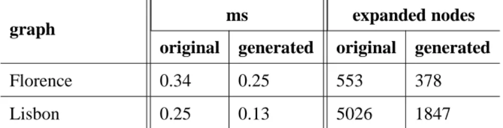
Our second approach computes tours of large Euclidean TSP instances from scratch, i. e., it does not require starting tours. In fact, computing multiple different good starting tours for theWorld TSPwith 1,904,711 cities is hardly realizable in reasonable time. The basic idea of our window based approach consists of splitting the bounding box of the vertices of the TSP instance in non-disjoint windows by moving a window frame across the bounding box of the vertices of the TSP instance with a step size of half the width (height) of the window frame (see Fig. 2). Thus each vertex is contained in up to four windows. Each window defines a sub-instance for which a good tour is computed, e. g., by Helsgaun’s LKH [2], independently of the neighboring sub-instances. Now, the approach is based on the assumption that an edge(u, w), which is contained in the same four windows and in each of the four

tours, has high probability to appear in an optimal tour of the original TSP instance – in some sense the four windows together reflect the surrounding area of (u, w)

with respect to the four directions. Such edges are declared as pseudo backbone edges (see Fig. 3(a)-3(c)). After the contraction of the maximum paths of pseudo backbone edges, the approach is iterated with monotonically increasing window frame. We applied the described algorithm to theWorld TSPand required about 4.75 days for computing from scratch a tour of length 7,569,766,108 which is only at most 0.7661% greater than the length of an optimum tour. Currently, our ap-proach is still dominated in some sense by LKH. By assigning the right values to the parameters, LKH computes a tour for the World TSPin less than two days which is at most 0,1174% greater than the length of an optimal tour [4].† How-ever, note that till now we have used only default parameters for LKH without any parameter tuning. By detailed parameter tuning – as done by Helsgaun – the win-dow frames of our approach can be chosen much larger which should lead to an improvement of the computed tours and running times.

References

[1] B. Goldengorin, G. J¨ager, and P. Molitor. Tolerances applied in combinatorial optimization. J. Comput. Sci. 2(9), 716-734, Science Publications, 2006.

† _{Note that the computation times, Helsgaun states in [2], do not include the computation}

(19)

Fig. 2. Illustration of the window based technique of splitting large TSP instances into sub-instances.

(a) Pseudo backbone edges found by the four top left-hand windows

(b) Pseudo backbone edges found in the current iteration.

(c)Constrained ETSP after con-traction of the paths shown in (b).

Fig. 3. Window based pseudo backbone computation and contraction.

[2] K. Helsgaun. An Effective Implementation of K-opt Moves for the Lin-Kernighan TSP heuristic. Writings on Computer Science 109, Roskilde Uni-versity, 2007.

[3] D. Richter, B. Goldengorin, G. J¨ager, and P. Molitor. Improving the Effi-ciency of Helsgaun’s Lin-Kernighan Heuristic for the Symmetric TSP. Proc.

of the 4th Workshop on Combinatorial and Algorithmic Aspects of Network-ing (CAAN), Lecture Notes in Comput. Sci. 4852, 99-111, 2007.

[4] K. Helsgaun. Private Communication, March 2009.

(20)

Efficient algorithms for the Double Traveling

Salesman Problem with Multiple Stacks

Marco Casazza,

a

Alberto Ceselli,

a

Marc Nunkesser

b

a_{Dept. of Information Technologies - University of Milan}

{marco.casazza, alberto.ceselli}@unimi.it

b_{Inst. of Theoretical Computer Science - ETH Z¨urich}

[email protected]

Key words: Traveling Salesman Problem, LIFO constraints, efficient algorithms

1. Introduction

Routing is a key issue in logistics, and has been deeply studied in the liter-ature; however, several practical applications require the loading of vehicles to be explicitly considered. The Double Traveling Salesman Problem with Multiple Stacks (DTSPMS) is one of the simplest examples of integrated routing and load-ing problem: two cities are given, in which N customers are placed. Items have to

be collected from the customers through a tour in the first city, and then delivered through a tour in the second city. During the pickup tour, the items have to be or-ganized in stacks on the back of the vehicle; the delivery operations can start only from the top of the stacks. The DTSPMS is NP-Hard, as it includes the TSP as a special case. Both heuristics [1] [2] and exact methods [3] have been proposed to solve it.

The main aim of this paper is to investigate on theoretical properties of the DT-SPMS; we also propose and test an efficient heuristic algorithm which exploits such properties.

2. Formulation and properties

The DTSPMS can be modeled as the following graph optimization problem. We are given a set of customers numbered1 . . . N and two (di-)graphs_G+_(N+_,_A+₎

and_G−(N−_,_A−_{) with weights c}+_and_c−_{respectively on the arcs. The former is the}

pickup graph and latter is the delivery graph. Both sets N+and N− consist of one vertexn+_i andn−_i for each customeri, and an additional vertex 0 which represents

a depot. Hence the number of vertices is the same in the two graphs. Each customer

i requires the pickup of an item in vertex n+i and the delivery of the same item in

(21)

pickup graph (resp. delivery graph). Each tour starts from and ends at the depot. Each tour has a cost, which is the cost for traveling from one vertex to the next, according to the order indicated by the permutation. Given two customersi and j,

we say thati precedes j on the pickup tour if n+

i appears to the left ofn+j in the

corresponding permutation. In a similar way,i precedes j on the delivery tour if n−_i

appears to the left ofn−j in the corresponding permutation.

The vehicle has a given numberS of stacks available for transportation. A loading

plan is a mappingl from each customer i to a pair (s, p), representing the

arrange-ment of the items in the stacks of the vehicle. In particular,l(i) = (s, p) if the item

of customeri occupies position p on stack s, with (s, 1) representing the bottom of

stacks.

Each stack actually represents a Last-In-First-Out structure: a loading plan is

feasi-ble with respect to a pickup tour (and vice versa) if, given any pair of customersi

andj such that i precedes j in the pickup tour, either l(i) = (s, p) and l(j) = (t, q)

with s 6= t, or p < q. That is, if item i is picked up before item j, i cannot be

placed on top ofj in the same stack. A similar definition holds for the delivery tour.

If i precedes j in both the pickup and the delivery tour, it must be l(i) = (s, p)

andl(j) = (t, q) with s _{6= t, and we say that customers i and j are incompatible.}

Hence, a solution of the DTSPMS is composed by two ingredients: a pair of pickup and delivery tours and a loading plan; such solution is feasible if the loading plan is feasible with respect to both tours.

In the following we show that, given one of the two ingredients of a feasible so-lution, the remaining one can be found in polynomial time. This holds in particular for an optimal solution. We present only a sketch of the proofs.

Problem (1): Given a pickup tour and a delivery tour, find a feasible loading

plan using the minimum number of stacks.

Proposition 1. Problem (1) can be solved in polynomial time.

We define a conflict graphC having one vertex for each customer, and one edge for

each pair of incompatible customers. Problem (1) can be re-stated as the problem of coloring graphC with the minimum number of colors: different colors represents

different stacks; since no adjacent vertices can take the same color in a feasible coloring, no incompatible customers can be assigned to the same stack. The or-der of the items inside each stack can be chosen according to their oror-der in one of the tours. We show that C is a permutation graph, which is a special case of

perfect graph. In these graphs coloring problems can be solved in polynomial time by means of flow computations [4]. As far as efficiency is concerned, we show that Problem (1) can be solved inO(N _{· logN) time by an adaptation of the algorithm}

presented in [4].

Problem (2): Given a loading plan, find a delivery tour which is feasible with

respect to the loading plan and has minimum cost.

Problem (3): Given a loading plan, find a pickup tour which is feasible with respect

to the loading plan and has minimum cost.

(22)

Proposition 2. Problem (2) and Problem (3) can be solved in polynomial time.

In fact, once a feasible loading plan is given, suppose to incrementally build partial delivery tours by choosing items on the top of the stacks. Let f (s1, . . . , sS, p) be

the minimum cost of a partial tour in whichs1 items are left in stack1, s2items are

left in stack2 and so on, and in which the item on the top of stack p is the next to

be delivered. Leti be the customer corresponding to the item on top of stack p; if i

is the first customer to be visited, then f (s1, . . . , sS, p) = c−0,i; otherwise, consider

any stackq, which has on top item j: f (s1, . . . , sS, p) = minq=1..S{f(s1, . . . , sq+ 1, . . . , sS, q) + c−j,i}. An optimal solution can be found in O(|N|S+1) time by

com-puting all the values forf () using dynamic programming recursion. Informally, the

computation can be repeated to solve Problem (3) by considering the items of each stack in reverse order.

However, given two random tours, it might not be possible to find a loading plan using at mostS stacks. Therefore we define as partial loading plan a loading

plan in which the items of a subset of customers do not appear, and we consider the following:

Problem (5): Given a pickup and a delivery tour, find a feasible partial loading plan

using at mostS stacks, including the maximum number of items.

Proposition 3. Problem (5) can be solved in polynomial time.

We build a graph having a vertex for each customer and two vertices for the depot (start and end), an arc between the vertex of each customer and the vertices of its compatible customers, between the start depot vertex and each customer vertex, and between each customer vertex and the end depot vertex. The start and end depot vertices are respectively a source and a sink ofS units of flow. We assign capacity 1

and cost0 to each arc, and cost−1 to each customer vertex. Problem (5) can be

re-stated as the problem of finding a minimum cost flow on a suitable modification of this graph. Informally, theS units of flow define sequences of customers included

in the same stack. Every time a vertex receives flow, the corresponding customer is inserted in a stack, and a value_{−1 is collected; therefore in an optimal solution the} maximum number of customers is included.

3. Algorithms

We elaborated on the previous results to obtain a heuristic algorithm for the DTSPMS. The algorithm works in five steps: (a) find a pickup tour and a deliv-ery tour (b) solve Problem (5), creating a feasible partial loading plan including the highest number of customers (c) solve Problem (2) and Problem (3) consider-ing only customers in the partial loadconsider-ing plan, creatconsider-ing optimal partial pickup and delivery tours (d) create a feasible DTSPMS solution by including the remaining customers in the stacks using a best insertion policy (e) create a candidate solution for the next iteration of the algorithm by including the remaining customers in the partial tours using a best insertion policy (f) repeat steps (b) – (f).

First we note that the number of customers which are inserted in the partial loading plan, which is found in step (b), is always non decreasing from one iteration to the

(23)

iterationk appear in the tours according to the order given by the partial loading

plan; our insertion algorithm do not change that order; hence, during iterationk + 1

it is always possible to rebuild the partial loading plan of iteration k. Therefore,

we stop the algorithm whenever no additional customer is inserted in the partial loading plan during step (c). In order to obtain a feasible solution in step (d), we consider the items which are not included in the loading plan in a random order. We try to place every item in each possible position in the stacks, and in each com-patible insertion point in the tours. Then, we place each item in the position of the loading plan giving minimum insertion cost. Instead, in order to obtain a candidate solution in step (e), we consider in a random order each customer whose item is not in the partial loading plan, and we perform a best insertion operation in both the pickup and delivery tours. We keep the best solution found in step (d) during the iterations of the main algorithm as final solution. In the literature, it is common to further constrain the problem by imposing a limit on the number of items which can be placed in the same stack. When such a constraint is imposed, during step (d) we remove from the partial loading plan each item exceeding the limit, and we care not to insert additional items in full stacks.

We implemented our heuristic algorithm in C, using MCF library for the flow sub-problems and CONCORDE to obtain tours in step (a). We considered the testbed of

10 instances involving 33 customers proposed in [1] and [3]. We run experiments

on a1.83GHz notebook ∗_{. As a benchmark, we considered the results of the HVNS}

metaheuristic [1], when let run for ten seconds. Our method provides in a fraction of a second solutions whose quality is about8% worse than those given by HVNS.

This highlights as a promising research direction to combine our algorithm with local search methods.

References

[1] A. Felipe, M.T. Ortuno and G. Tirado (2008) Neighborhood structures to solve the double TSP with multiple stacks using local search. FLINS Proceedings, Madrid, September 21–24 2008

[2] H. Petersen and O. Madsen. (2008) The double travelling salesman problem with multiple stacks - formulation and heuristic solution approaches. Euro-pean Journal of Operational Research, forthcoming

[3] H. Petersen, C. Archetti and M.G. Speranza (2008) Exact Solutions to the double TSP with multiple stacks. Tech. rep, University of Brescia

[4] A. Brandst¨adt (1992) On Improved Time Bounds for Permutation Graph Problems. Lecture Notes in Computer Science 657

∗ _{A full table is available at: http://www.dti.unimi.it/}_{∼ceselli/DTSPMS.thml}

(24)

The Parking Warden Tour Problem

Maurizio Bruglieri,

a

Alberto Colorni,

a

Alessandro Lu´e

b

a_{INDACO, Politecnico di Milano, via Durando 38/a, 20158 Milano, Italy}

{maurizio.bruglieri,alberto.colorni}@polimi.it

b_{POLIEDRA, Politecnico di Milano, via Garofalo 39, 20133 Milano, Italy}

[email protected]

Key words: irregular parking, parking warden tour, arc routing problem.

1. Introduction

Irregular parking is a scourge for most of the Italian cities and in most of the cases enforcement ([6]) is not effective. Unfortunately, municipalities have lim-ited resources to hire a sufficient number of parking wardens, and the tours and schedule of the existing wardens are not planned using quantitative models. For the municipality of Como (Italy), we are studying how to re-configure the park-ing system, considerpark-ing both pricpark-ing and organizational aspects. Within this study, we developed a model to improve the level of efficiency of the parking enforce-ment optimizing the parking warden tours. The problem is the following. The team of parking wardens, the city road network, the link travel time, and the estimated profit deriving from the sanctions applied to the cars irregularly parked are given. We want to determine the tour of each warden (that is a cycle where both vertices and edges may be repeated and having total duration less than the warden service time), with the aim of maximizing the total profit collected. In the literature, we do not find mathematical models that face this problem. This problem differs from the Profitable Arc Tour problem [1] since in the latter both the arc profits and costs are fixed whereas in our problem they depend on the moment of the day (the average number of irregular parked cars can vary during the day) and on the time passed from the previous inspection of a warden (the profit on a link slumps to zero if a warden has just visited this link). This peculiarity occurs in other different rout-ing problems. For instance, in the snowplough vehicles routrout-ing problem the profit collected is the amount of snow removed, which depends on the time passed from the previous transit of a snowplough, supposing that it is snowing during the op-erations. At the best of our knowledge ( [1], [4] [5]), this is the first study of an arc routing problem where the arc profit depends also on the solution itself. For

(25)

this new arc routing problem, we present a MILP formulation from which we also develop a simple but effective heuristic approach.

2. Graph representation of the problem

Since the wardens inspect the road network by foot, the problem can be mod-elled by way of an undirected graph where each edge represents a road link that can be travelled in both the directions. In each road link the cars can be parked from one to four sides according to the width of the road and the presence or not of a traffic island. Each side is visited by the wardens in different moments, except the two sides of the traffic islands. Therefore, we have to duplicate the ending vertices of the original road links if they have two parking sides or triplicate the ending ver-tices if in addition there is a traffic island, to avoid parallel edges. The edges linking the copies of the same vertex represent the action of crossing the road to change the side and no profit is associated to them.

3. Mixed Integer Linear Programming formulation

Beside the undirected graphG = (V, E) described in the previous section, we

suppose also given the following data:

W = parking warden set T = parking warden service time ce= travel time by foot of edgee q = time needed to sanction one car p = profit for one irregularly parked car

se= estimation of irregularly parked cars on edgee Re= estimation of turn-over time on edgee

We assume that a team of wardens is available at a single depot, represented by vertex 0, and they have to come back to depot at the end of the service. Moreover we assume that the profit of an edgee slumps to zero when such edge is visited

by a warden. Afterwards, the profit increases linearly from 0 topse until the

turn-over timeReis reached, after which it remains constant until the next visit. Under

these assumptions, we state that the Parking Warden Tour Problem (PWTP) can be modeled by way of the following Mixed Integer Linear Program (MILP), whereK

is an upper bound on the number of edges that the wardens can visit along their tour (for instanceK = _minT

e∈Ece ) andδ(0) denotes the edges incident to the depot.

(26)

maxP_w∈WPK_k=1πkw (3.1) PK

k=1 P

e∈E_P(cexekw+ qsezekw)≤ T ∀w ∈ W (3.2)

e∈δ(0)xe1w= 1 ∀w ∈ W (3.3) P e∈Exekw≤ 1 ∀k = 2,...,K, ∀w ∈ W (3.4) v01w= 1 ∀w ∈ W (3.5) PK k=2v0kw= 1 ∀w ∈ W (3.6) P i∈Vvikw≤ 1 ∀k = 2,...,K + 1, ∀w ∈ W (3.7) P i:{i,j}∈Evik+1w≥ vjkw ∀j ∈ V, ∀k = 1,...,K, ∀w ∈ W (3.8) P i∈N PK+1 k0=k+1vik0w≤ (K − k + 1) (1 − v0kw) ∀k = 2,...,K, ∀w ∈ W (3.9)

xekw≥ vikw+ vjk+1w− 1 ∀e = {i, j}∈ E, ∀k = 1,...,K, ∀w ∈ W (3.10)

xekw≤ vikw ∀e = {i, j}∈ E, ∀k = 1,...,K, ∀w ∈ W (3.11)

xekw≤ vjk+1w ∀e = {i, j}∈ E, ∀k = 1,...,K, ∀w ∈ W (3.12)

zekw≤ xekw ∀e = {i, j}∈ E, ∀k = 1,...,K, ∀w ∈ W (3.13)

t1w= 0 ∀w ∈ W (3.14)

tkw≥ tk−1w+P_e∈E(cexek−1w + qsezek−1w)

∀k = 2,...,K + 1, ∀w ∈ W (3.15) πkw≤ pP_e∈Esezekw ∀k = 1,...,K, ∀w ∈ W (3.16) π_k00_w≤ pse t_{k00 w}−t_{k0 w} Re + pS(2− zek00w− zek0w+ k_X00−1 k=k0₊₁ zekw) ∀e ∈ E, ∀k0, k00= 1,...,K : k00> k0,∀w ∈ W (3.17) π_k00_w00 ≤ pse t k00 w00−tk0 w0 Re +pS(1 + T Re )(3− zek00_w00− z_ek0_w0− y_k0_k00_w0_w00) ∀e ∈ E, ∀k0, k00= 1,...,K,∀w0, w00∈ W : w0< w00 (3.18) π_k0_w0 ≤ pse t k0 w0−tk00 w00 Re +pS(1 + T Re )(2− zek00w00− zek0w0− yk0k00w0,w00) ∀e ∈ E, ∀k0, k00= 1,...,K,∀w0, w00∈ W : w0< w00 (3.19) y_k0_k00_w0_w00 ≤ 3 + t_k00_w00− t_k0_w0 T − zek0_w0 − z_ek00_w00 ∀e ∈ E, ∀k0, k00= 1,...,K,∀w0,w00∈ W : w0< w00 (3.20) y_k0_k00_w0_w00≥ −2 + t_k00_w00− t_k0_w0 T + zek0w0 + zek00w00 ∀e ∈ E, ∀k0, k00= 1,...,K,∀w0,w00∈ W : w0< w00 (3.21) xekw≥ 0 ∀e ∈ E, ∀k = 1, ...,K, ∀w ∈ W (3.22) yk0k00w0w00∈ {0, 1} ∀k0, k00= 1, ...,K,∀w0, w00∈ W : w0< w00 (3.23) vikw∈ {0, 1} ∀i ∈ V, ∀k = 1, ...,K + 1, ∀w ∈ W (3.24) zekw∈ {0, 1} ∀e ∈ E, ∀k = 1, ...,K, ∀w ∈ W (3.25) πkw≥ 0 ∀k = 1, ...,K, ∀w ∈ W (3.26) 0≤ tkw≤ T ∀k = 1, ...,K + 1, ∀w ∈ W (3.27)

Variablesπkw model the profit collected by wardenw when visiting the k-th

edge of his/her tour: these variables are settled by constraints (3.16) and bybig-M

constraints (3.17), (3.18) and (3.19), whereS = maxe∈Ese. Therefore the objective

function (3.1) models the maximization of the total collected profit.

(27)

otherwise. Thanks to constraints (3.10), (3.11) and (3.12), variablesxekware binary

although not directly constrained to be so: in particular they are equal to 1 if edge

e is the k-th edge visited by warden w in his/her tour (independently on the fact

that its profit is collected or not), are equal to 0 otherwise. Indeed (3.10), (3.11) and (3.12) can be seen as McCormick linearization constraints ([3]) imposing that variablesxekw have the same behaviour of bilinear termsvikwvjk+1wwheree is the

edge linking verticesi and j.

Variableszekware equal to 1 if edgee is the k-th edge visited by warden w in his/her

tour and its profit is collected, are equal to 0 otherwise.

Variablestkw model the time instant when thek-th edge is visited by warden w;

variablesyk0_k00_w0_w00model the precedence relationships in the visit of the same edge by different wardens: in particular when thek0_{-th edge travelled by warden}_w0 _and

thek00-th edge travelled by wardenw00 coincide, such variables are equal to 1 ifw00

precedesw0 _{, are equal to 0 otherwise.}

4. Some computational results

We notice that MILP (1)-(27) involves O(|E|K|W | + K2_{|W |}2_{) binary}

vari-ables andO(_|E|K2_{|W |}2_{) linear constraints, therefore in practice we cannot think}

of applying this model directly to the whole team of wardens, unless to consider just small instances. Anyway from the MILP model we can build a simple but ef-fective heuristic approach. It consists in iteratively solving, with the MILP (1)-(27),

|W | instances of PWTP with one warden, where, at each iteration, the profit

collec-tion of the edges already visited with profit in the previous iteracollec-tions, is forbidden. We have implemented the MILP (1)-(27) in AMPL [2] and considered random in-stances with number of vertices between 10 and 50, number of edges between 30 and 150 and up to 4 wardens. The preliminary computational results obtained with CPLEX11.0 solver show that the heuristic is able to find a solution always in few seconds, whereas the MILP can require hundreds of seconds up to 2 wardens and also several hours for 4 wardens. Concerning the solution quality, we have found an average percentage gap between the heuristic and the optimal solution of about 5.8%.

References

[1] D. Feillet, P.Dejax, M.Gendreau. The Profitable Arc Tour Problem: Solution with a Branch-and-Price Algorithm. Transportation Science, 39(4):539–552, 2005.

[2] R. Fourer and D. Gay The AMPL Book. Duxbury Press, Pacific Grove, 2002. [3] G.P. McCormick. Computability of global solutions to factorable nonconvex

(28)

programs: part I-convex underestimating problems. Mathematical

Program-ming, 10:146–75, 1976.

[4] N. Perrier, A. Langevin, J.F. Campbell. A survey of models and algorithms for winter road maintenance. Part IV: Vehicle routing and fleet sizing for plowing and snow disposal. Computers & Operations Research, 34:258–294, 2007. [5] N. Perrier, A. Langevin, A. Amaya. Vehicle routing for urban snow plowing

operations. Les Cahiers du GERAD, G-2006-33, 2006.

[6] R. Petiot Parking enforcement and travel demand management. Transport

(29)

(30)

Graph Theory I

Lecture Hall B

(31)

(32)

On Self-Duality of Branchwidth

in Graphs of Bounded Genus ?

Ignasi Sau,

a

Dimitrios M. Thilikos

b

a_{Mascotte project INRIA/CNRS/UNSA, Sophia-Antipolis, France; and Graph Theory and}

Comb. Group, Applied Maths. IV Dept. of UPC, Barcelona, Spain.

b_{Department of Mathematics, National Kapodistrian University of Athens, Greece.}

Abstract

A graph parameter is self-dual in some class of graphs embeddable in some surface if its value does not change in the dual graph more than a constant factor. Self-duality has been examined for several width-parameters, such as branchwidth, pathwidth, and treewidth. In this paper, we give a direct proof of the self-duality of branchwidth in graphs embedded in some surface. In this direction, we prove that bw(G∗)_{≤ 6 · bw(G) + 2g − 4 for any graph} G embedded in a surface of Euler genus g.

Key words: graphs on surfaces, branchwidth, duality, polyhedral embedding.

1. Preliminaries

A surface is a connected compact 2-manifold without boundaries. A surfaceΣ

can be obtained, up to homeomorphism, by adding eg(Σ) crosscaps to the sphere. eg(Σ) is called the Euler genus of Σ. We denote by (G, Σ) a graph G embedded

in a surface Σ. A subset of Σ meeting the drawing only at vertices of G is called G-normal. If an O-arc is G-normal, then we call it a noose. The length of a noose is

the number of its vertices. Representativity, or face-width, is a parameter that quan-tifies local planarity and density of embeddings. The representativityrep(G, Σ) of

a graph embedding(G, Σ) is the smallest length of a non-contractible noose in Σ.

We call an embedding(G, Σ) polyhedral if G is 3-connected and rep(G, Σ) _{≥ 3.}

See [7] for more details. For a given embedding (G, Σ), we denote by (G∗_{, Σ) its}

dual embedding. Thus G∗ is the geometric dual ofG. Each vertex v (resp. face r)

in(G, Σ) corresponds to some face v∗_{(resp. vertex}_r∗_{) in}_(G∗_{, Σ). Also, given a set}

X _{⊆ E(G), we denote as X}∗ _{the set of the duals of the edges in}_X.

? This work has been supported by IST FET AEOLUS, COST 295-DYNAMO, and by the Project “Kapodistrias” (AΠ 02839/28.07.2008) of the National and Kapodistrian Univer-sity of Athens (project code: 70/4/8757).

(33)

Given a graphG and a set X _{⊆ E(G), we define ∂X = (}S_e_∈Xe)_∩(S_e_∈E(G)\Xe)

(notice that∂X = ∂(E(G)_{\X)). A branch decomposition (T, µ) of a graph G}

con-sists of an unrooted ternary treeT (i.e., all internal vertices are of degree three) and

a bijectionµ : L _{→ E(G) from the set L of leaves of T to the edge set of G. For}

every edgef =_{t1, t2} of T we define the middle set mid(e) ⊆ V (G) as follows:

LetL1 be the leaves of the connected component ofT \ {e} that contain t1. Then

mid(e) = ∂µ(L1). The width of (T, µ) is defined as max{|mid(e)|: e ∈ T }. An

optimal branch decomposition ofG is defined by a tree T and a bijection µ which

give the minimum width, called the branchwidth ofG, and denoted by bw(G).

SupposeG1andG2are graphs with disjoint vertex-sets andk ≥ 0 is an integer.

For i = 1, 2, let Wi ⊆ V (Gi) form a clique of size k and let G0i (i = 1, 2) be

obtained fromGi by deleting some (possibly none) of the edges fromGi[Wi] with

both endpoints inWi. Consider a bijectionh : W1 → W2. We define a clique-sum G1 ⊕ G2 ofG1 and G2 to be the graph obtained from the union of G01 andG02 by

identifyingw with h(w) for all w ∈ W1.

Let _{G be a class of graphs embeddable in a surface Σ. We say that a graph}

parameterCRRAP is (c, d)-self-dual on _{G if for every graph G ∈ G and for its}

geometric dualG∗_,_{CRRAP (G}∗₎_{≤ c · CRRAP (G) + d. Results concerning}

self-duality of pathwidth can be found in [4; 1]. Branchwidth is(1, 0)-self-dual in planar

graphs that are not forests [9], while analogous results have been proven for other parameters such as pathwidth [3; 1] and treewidth [5; 2; 6]. In this note, we give a proof that branchwidth is(6, 2g_{− 4)-self-dual in graphs of Euler genus at most} g. We also believe that our result can be considerably improved. In particular, we

conjecture that branchwidth is(1, g)-self-dual.

2. Self-duality of banchwidth

If(G, Σ) is a polyhedral embedding, then the following proposition follows by

an easy modification of the proof of [4, Theorem 1].

Proposition 2.1. Let(G, Σ) and (G∗_{, Σ) be dual polyhedral embeddings in a}

sur-face of Euler genusg. Then bw(G∗₎_{≤ 6 · bw(G) + 2g − 4.}

In the sequel, we focus on generalizing Proposition 2.1 to arbitrary embeddings. For this we first need some technical lemmata, whose proofs are easy or well known, and omitted in this extended abstract. Note that the removal of a vertex inG

corre-sponds to the contraction of a face inG∗, and viceversa.

Lemma 2.2. The removal of a vertex or the contraction of a face from an

embed-ded graph decreases its branchwidth by at most 1.

Lemma 2.3. (Fomin and Thilikos [3]) LetG1andG2be graphs with one edge or

one vertex in common. Then bw(G1∪ G2)≤ max{bw(G1), bw(G2), 2}.

Theorem 2.4. Let (G, Σ) be an embedding with g = eg(Σ). Then bw(G∗₎ _≤

(34)

6_{· bw(G) + 2g − 4.}

Proof. The proof uses the following procedure that applies a series of cutting

operations to decomposeG into polyhedral pieces plus a set of vertices whose size

is linearly bounded by eg(Σ). The input is the graph G and its dual G∗_embedded

inΣ.

1. Set_{B = {G}, and B}∗ ={G∗_{} (we call the members of B and B}∗_blocks).

2. If(G, Σ) has a minimal separator S with _{|S| ≤ 2, let C}1, . . . , Cρbe the

con-nected components ofG[V (G)_{\ S] and, for i = 1, . . . , ρ, let G}i be the graph

obtained by G[V (Ci)∪ S] by adding an edge with both endpoints in S in

the case where _{|S| = 2 and such an edge does not already exist (we refer to} this operation as cuttingG along the separator S). Notice that a (non-empty)

separator S of size at most 2 corresponds to a non-empty separator S∗ of

G∗_{, and let} _G∗

i, i = 1, . . . , ρ be the graphs obtained by cutting G∗ along S∗.

We say that each Gi (resp G∗i) is a block of G (resp. G∗) and notice that

each G and G∗ is the clique sum of its blocks. Therefore, from Lemma 2.3,

bw(G∗₎ _{≤ max{2, max{bw(G}∗

i) | i = 1, . . . , ρ}} (1). Observe that we

may assume that for each i = 1, . . . , ρ, Gi and G∗i are embedded in a

sur-faceΣi such thatGi is the dual ofG∗i and eg(Σ) =

P

i=1,...,ρeg(Σi). Notice

that bw(Gi) ≤ bw(G), i = 1, . . . , ρ (2), as the possible edge addition does

not increase the branchwidth, since each block of G is a minor of G. We set B ← B \ {G} ∪ {G1, . . . , Gρ} and B∗ ← B∗ \ {G∗} ∪ {G∗1, . . . , G∗ρ}.

3. If (G, Σ) has a non-contractible and non-surface-separating noose meeting a

set S with_{|S| ≤ 2, let G}0 _{= G[V (G)}_{\ S] and let F be the set of of faces in}

G∗ corresponding to the vertices inS. Observe that the obtained graph G0has an embedding to some surfaceΣ0 _{of Euler genus strictly smaller than}_{Σ that,}

in turn, has some dual G0∗ _in_Σ0_{. Therefore eg}_(Σ0_{) < eg(Σ). Moreover, G}0∗

is the result of the contraction in G∗ of the_{|S| faces in F . From Lemma 2.2,}

bw(G∗₎ _{≤ bw(G}0∗_{) +}_{|S| (3). Set B ← B \ {G} ∪ {G}0_{} and B}∗ _{← B}∗ _\

{G∗_{} ∪ {G}0∗_}.

4. Apply (recursively) Steps 2–4 for each blockG∈ B and its dual.

We now claim that before each recursive call of Steps 2–4, it holds that bw(G∗₎_≤

6_{· bw(G) + 2eg(Σ) − 4. The proof uses descending induction on the the distance}

from the root of the recursion tree of the above procedure. Notice that all embed-dings of graphs in the collections_{B and B}∗constructed by the above algorithm are polyhedral, except from the trivial case that they are just cliques of size 2. Then the theorem follows directly from Proposition 2.1.

Suppose that G (resp. G∗_{) is the clique sum of its blocks} _G

1, . . . , Gρ (resp. G∗

1, . . . , G∗ρ) embedded in the surfacesΣ1, . . . , Σρ(Step 2). By induction, we have

that bw(G∗_i)≤ 6 · bw(Gi) + 2eg(Σi)− 4, i = 1, . . . , ρ and the claim follows from

(35)

Suppose now (Step 3) thatG (resp. G∗_{) occurs from some graph}_G0 _(resp._G0∗₎

embedded in a surface Σ0 _{where eg}_(Σ0_{) < eg(Σ) after adding the vertices in S}

(resp.S∗_{). From the induction hypothesis, bw}_(G0∗₎_{≤ 6 · bw(G}0_{) + 2eg(Σ}0₎_{− 4 ≤}

6_{· bw(G}0_{) + 2eg(Σ)}_{− 2 − 4 and the claim follows easily from Relation (3) as}

|S| ≤ 2 and bw(G0₎_{≤ bw(G).}

3. Recent results and a conjecture

Very recently Mazoit [6] proved that treewidth is a(1, g + 1)-self-dual

param-eter in graphs embeddable in surfaces of Euler genusg. Using that the branchwidth

and the treewidth of a graphG, with_{|E(G)| ≥ 3, satisfy bw(G) ≤ tw(G) + 1 ≤} 3

2bw(G) [8], this implies that bw(G∗) ≤

3

2bw(G) + g + 2, improving the

con-stants of Theorem 2.4. We believe that an even tighter self-duality relation holds for branchwidth and hope that the approach of this paper will be helpful to settle the following conjecture.

Conjecture 1. If G is a graph embedded in some surface Σ, then bw(G∗) ≤

bw(G∗_{) + eg(Σ).}

References

[1] O. Amini, F. Huc, and S. P´erennes. On the Pathwidth of Planar Graphs. SIAM

Journal on Discrete Mathematics, 2009. To appear.

[2] V. Bouchitt´e, F. Mazoit, and I. Todinca. Chordal embeddings of planar graphs.

Discrete Mathematics, 273(1-3):85–102, 2003. EuroComb’01 (Barcelona).

[3] F. V. Fomin and D. M. Thilikos. Dominating Sets in Planar Graphs: Branch-Width and Exponential Speed-Up. SIAM Journal on Computing, 36(2):281– 309, 2006.

[4] F. V. Fomin and D. M. Thilikos. On self duality of pathwidth in polyhedral graph embeddings. Journal of Graph Theory, 55(1):42–54, 2007.

[5] D. Lapoire. Treewidth and duality for planar hypergraphs, 1996:

http://www.labri.fr/perso/lapoire/papers/dual planar treewidth.ps. [6] F. Mazoit. Tree-width of graphs and surface duality. To appear in DIMAP

workshop on Algorithmic Graph Theory (AGT), Warwick, U.K., March 2009.

[7] B. Mohar and C. Thomassen. Graphs on surfaces. John Hopkins University Press, 2001.

[8] N. Robertson and P. Seymour. Graph minors. X. Obstructions to Tree-decomposition. J. Comb. Theory Series B, 52(2):153–190, 1991.

[9] P. Seymour and R. Thomas. Call routing and the ratcatcher. Combinatorica, 14(2):217–241, 1994.

(36)

A simple linear-time recognition algorithm

for weakly quasi-threshold graphs

1

Stavros D. Nikolopoulos, Charis Papadopoulos

Department of Computer Science, University of Ioannina

P.O.Box 1186, GR-45110 Ioannina, Greece

{stavros,charis_}@cs.uoi.gr

Abstract

Weakly quasi-threshold graphs form a proper subclass of the well-known class of cographs by restricting the join operation. In this paper we characterize weakly quasi-threshold graphs by a finite set of forbidden subgraphs: the class of weakly quasi-threshold graphs co-incides with the class of{P4, co-(2P3)}-free graphs. Moreover we give the first linear-time

algorithm to decide whether a given graph belongs to the class of weakly quasi-threshold graphs, improving the previously known running time. Based on the simplicity of our recognition algorithm, we can provide certificates of membership (a structure that charac-terizes weakly quasi-threshold graphs) or non-membership (forbidden induced subgraphs) in additionalO(n) time. Furthermore we give a linear-time algorithm for finding the largest induced weakly quasi-threshold subgraph in a cograph.

1. Introduction

The well-known class of cographs is recursively defined by using the graph op-erations of ‘union’ and ‘join’ [4]. Bapat et al. [1], introduced a proper subclass of cographs, namely the class of weakly quasi-threshold graphs, by restricting the join operation and studied their Laplacian spectrum. In the same work they proposed a quadratic-time algorithm for recognizing such graphs. Here we characterize the class of weakly quasi-threshold graphs by the class of graphs having noP4

(chord-less path on four vertices) or co-(2P3) (the complement of two disjoint P3’s). This

characterization also shows that the complement of a weakly quasi-threshold graph is not necessarily weakly quasi-threshold graph. Moreover we give a tree represen-tation for such graphs, similar to the cotrees for cographs, and propose a linear-time recognition algorithm.

(37)

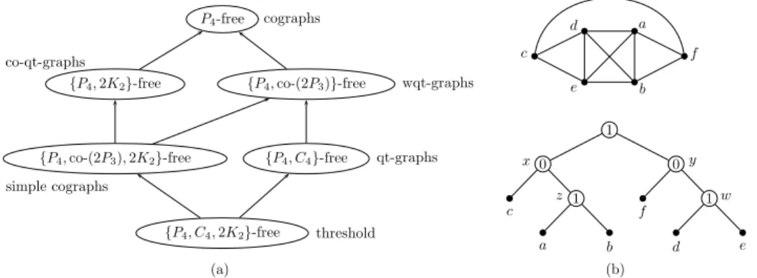
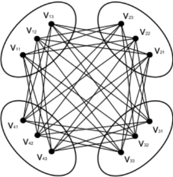
cographs P4-free

co-qt-graphs

{P4,2K2}-free {P4,co-(2P3)}-free wqt-graphs

simple cographs

{P4,co-(2P3), 2K2}-free {P4, C4}-free qt-graphs

threshold {P4, C4,2K2}-free c d a f e b 1 0 x 0 y c 1 z f 1 w a b d e (a) (b)

Fig. 1. (a) Subclasses of cographs and (b) a co-(2P3) and its cotree.

The class of cographs coincides with the class of graphs having no inducedP4

[5]. There are several subclasses of cographs. Trivially-perfect graphs, also known as quasi-threshold graphs, are characterized as the subclass of cographs having no inducedC4(chordless cycle on four vertices), that is, such graphs are{P4, C4

}-free graphs, and are recognized in linear time [3; 6]. Another interesting subclass of cographs are the_{P4, C4, 2K2}-free graphs known as threshold graphs, for which

there are several linear-time recognition algorithms [3; 6]. Clearly every threshold graph is trivially-perfect but the converse is not true. Gurski introduced the class of

{P4, co-(2P3), 2K2}-free graphs in his study of characterizing graphs of certain

re-stricted clique-width [7]. Together with the class of weakly quasi-threshold graphs (that are exactly the class of_{P4, co-(2P3)}-free graphs as we show in this paper),

we obtain the inclusion properties for the above families of graphs that we depict in Figure 1 (a).

For undefined terminology we refer to [3; 6]. A vertex x of G is universal if

NG[x] = V (G) and is isolated if it has no neighbors in G. Two vertices x, y of G are

called false twins ifNG(x) = NG(y). A clique is a set of pairwise adjacent vertices

while an independent set is a set of pairwise non-adjacent vertices. A chordless cycle onk vertices is denoted by Ck and a chordless path onk vertices is denoted

byPk. The complement of the graph consisting of two disjointP3’s is denoted by

co-(2P3). Given two vertex-disjoint graphs G1 = (V1, E1) and G2 = (V2, E2), their

union isG1∪ G2 = (V1∪ V2, E1∪ E2). Their join G1+ G2 is the graph obtained

fromG1∪ G2by adding all the edges between the vertices ofV1andV2. The class

of cographs, also known as complement reducible graphs, is defined recursively as follows:

(c1) a single vertex is a cograph;

(c2) ifG1 andG2 are cographs, thenG1∪ G2is also a cograph;

(c3) ifG1 andG2 are cographs, thenG1+ G2 is also a cograph.

The class of cographs coincides with the class of P4-free graphs [5]. Along with

other properties, it is known that cographs admit a unique tree representation, called a cotree [4]. For a cographG its cotree, denoted by T (G), is a rooted tree having O(n) nodes. The vertices of G are precisely the leaves of T (G) and every internal

node ofT (G) is labelled by either 0 (0-node) or 1 (1-node). Two vertices are

(38)

cent inG if and only if their least common ancestor in T (G) is a 1-node. Moreover,

if G has at least two vertices then each internal node of the tree has at least two

children and any path from the root to any node of the tree consists of alternating

0- and 1-nodes. The complement of any cograph G is a cograph and the cotree of

the complement ofG is obtained from T (G) with inverted labeling on the internal

nodes ofT (G). Note that we distinguish between vertices of a graph and nodes of a

tree. Cographs can be recognized and their cotrees can be computed in linear time [5; 8; 2].

2. A characterization of weakly quasi-threshold graphs

Bapat et al., introduced in [1] the class of weakly quasi-threshold graphs (or

wqt graphs for short) and defined the given class as follows:

(w1) a single vertex is a wqt graph;

(w2) ifG1 andG2are wqt graphs thenG1∪ G2is a wqt graph;

(w3) ifG is a wqt then adding a universal vertex in G results in a wqt graph;

(w4) ifG is a wqt graph then adding a vertex in G having the same neighborhood

with a vertex ofG results in a wqt graph.

By definition the class of cographs and wgt graphs have certain similarities. Clearly every wqt graph is a cograph but the converse is not true. Properties c1,c2 and w1,w2 completely coincide, whereas properties w3–w4 correspond to a restricted version of c3. Moreover it follows that in a connected wqt graph there is either a universal vertex or a false twin. Then it is not difficult to see that the class of wqt graphs is closed under taking induced subgraphs, that is, the class of wqt graphs is

hereditary.

Lemma 2.1. The class of wqt graphs can be defined recursively as follows:

(a1) an edgeless graph is a wqt graph; (a2) if G1 and G2 are wqt graphs then G1 ∪ G2 is a wqt graph; (a3) ifG is a wqt graph and H is an edgeless graph then G + H is a wqt graph.

Proof. Properties w2 and a2 are exactly the same. By properties w1 and w2

we have that edgeless graphs are wqt graphs. We need to show that property a3 can substitute both properties w3–w4. If G is a wqt graph and H is an edgeless

graph then the graph G + H is obtained by first adding a universal vertex in G

and then by the addition of false twins. Hence G + H is a wqt graph. For the

converse let G be a connected wqt graph. First observe that G can be reduced

to a disconnected wqt graph G[A] by repeatedly removing a universal vertex or

a false twin vertex. Let S be a set of the removal vertices. Let xn, . . . , xk be an

order ofS where xi is either universal or false twin inGi = G[{xi, . . . , xk} ∪ A],

n _{≤ i ≤ k. We show that there is such an order of {x}n, . . . , xk} where all the false

twin vertices appear consecutive. If there is a universal vertexxj between two false

(39)

between two false twin vertices and obtain an order of the vertices ofS where the

false twin vertices appear consecutive. Observe that the set of the false twin vertices induces an edgeless graph inG. Thus the join operation between a wqt graph and

an edgeless graph is sufficient to construct a connected wqt graph.

Next we give a characterization of weakly quasi-threshold graphs through for-bidden subgraphs based on Lemma 2.1.

Theorem 2.1. A graphG is weakly quasi-threshold if and only if G does not

con-tain anyP4or co-(2P3) as induced subgraphs.

3. A linear-time recognition algorithm

In this section we give a linear-time algorithm for deciding whether an arbitrary graph is wqt. LetG be the input graph. We first apply the linear-time recognition

algorithm for checking whetherG is a cograph [5]. If G is not a cograph then we

know that G is not a wqt graph as it contains a P4. Otherwise G admits a cotree T (G) that can be constructed in linear time [5; 8]. Now it suffices to efficiently

check an induced co-(2P3) on G by using the cotree T (G). For that purpose, we

modifyT (G) and obtain T∗ _from_{T (G) by applying the following two operations:}

(i) delete the subtree rooted at a 0-node having only leaves as children and (ii) remove a leaf that has 1-node as parent. Next we check if every 1-node inT∗ has at most one child. In case of an affirmative answer we output thatG is a wqt graph;

otherwise, we output that G is not a wqt graph. Correctness of the algorithm is

based on the following lemma.

Lemma 3.1. LetG be a cograph and let T∗ _{be its modified cotree. Then}_{G is wqt}

graph if and only if every 1-node ofT∗_{has at most one child.}

Theorem 3.1. Weakly quasi-threshold graphs can be recognized in_{O(n+m) time.}

Furthermore given a graphG there is an_{O(n + m) algorithm that reports either an}

inducedP4 or co-(2P3) of G whenever G is not a weakly quasi-threshold graph.

As already mentioned every wqt graph is a cograph but the converse is not neces-sarily true. We show that the problem of removing the minimum number of vertices from a cograph so that the resulting graph is wqt can be done in linear time. Note that the proposed algorithm can serve as a recognition algorithm as well. LetT (G)

be the cotree ofG and let T∗_{be the modified cotree. Our algorithm starts by}

travers-ing bothT (G) and T∗ _{from the leaves to the root and computes for each node of} T (G) a largest induced wqt subgraph; the one computed at the root of T (G)

pro-vides the largest induced wqt subgraph of G. The computed graph is represented

by a cotreeT0 _{that we construct during the traversal of} _{T (G). Let H}

u be the

in-duced subgraph ofG corresponding to the leaves of the subtree rooted at a node u

ofT (G). Every time the algorithm visits a node u of T (G) it computes the triple

(40)

(n(u), MC(u), MI(u)) where n(u) is the number of vertices of Hu, MC(u) is the

maximum clique of Hu, and MI(u) is the maximum independent set of Hu. Let u1, u2, . . . , uk be the children ofu in T (G). If u is a 0-node or a 1-node with at

most one child then the algorithm assigns tou the correct triple by Lemma 3.1 and

copies nodeu in T0_{. If}_{u is a 1-node and u has at least two children in T}∗ _{then we}

need to modify the subtree rooted at u. Let u∗

1, u∗2, . . . , u∗` be the children of u in T∗_{; note that each child}_u∗

1 is a 0-node,1 ≤ i ≤ `. Based on Lemma 3.1 we

mod-ify every subtree in T (G) rooted at u∗

i except that u∗p having the maximum value

amongmin{n(u∗

i)− |MC(u∗i)|, n(u∗i)− |MI(u∗i)|}. For every other node u∗j 6= u∗p

we do the following operations: if_|MC(u∗_j)_{| > |MI(u}∗

j)| then we delete the subtree

rooted atu∗

j and add the vertices of MC(u∗j) as children of u; otherwise we remove

the nodes of the subtree rooted at u∗

j and add the vertices of MI(u∗j) as children of u∗j.

Theorem 3.2. Given a cograph G there is an _{O(n + m) algorithm that finds a}

largest induced weakly quasi-threshold subgraph ofG.

References

[1] R.B. Bapat, A.K. Lal, and S. Pati. Laplacian spectrum of weakly quasi-threshold graphs. Graphs and Combinatorics, 24:273–290, 2008.

[2] A. Bretscher, D. Corneil, M. Habib, and C. Paul. A simple linear time LexBFS co-graph recognition algorithm. SIAM Journal on Discrete Mathematics, 22:1277–1296, 2008.

[3] A. Brandst¨adt, V.B. Le, and J.P. Spinrad. Graph Classes: A Survey. SIAM Mono-graphs on Discrete Mathematics and Applications, 1999.

[4] D.G. Corneil, H. Lerchs, and L.K. Stewart. Complement reducible graphs. Discrete

Applied Mathematics, 3:163–174, 1981.

[5] D.G. Corneil, Y. Perl, and L.K. Stewart. A linear recognition algorithm for cographs.

SIAM Journal on Computing, 14:926–934, 1985.

[6] M. C. Golumbic. Algorithmic Graph Theory and Perfect Graphs. Second edition. Annals of Discrete Mathematics 57. Elsevier, 2004.

[7] F. Gurski. Characterizations for co-graphs defined by restricted NLC-width or clique-width operations. Discrete Mathematics, 306:271–277, 2006.

[8] M. Habib and C. Paul. A simple linear time algorithm for cograph recognition.

(41)

From Sainte-Lagu¨e to Claude Berge — French graph

theory in the twentieth century ??

Harald Gropp

a

a_{Hans-Sachs-Str. 6, D-65189 Wiesbaden}

[email protected]

Key words: graph theory, Berge graph

1. Introduction

Dedicated to CLAUDE BERGE (1926-2002), mathematician and man of culture

In 1926 the zeroth book on graph theory was published by A. Sainte-Lagu¨e [9]. It collects the knowledge on graphs at this early stage and particularly focusses on the French development of this new field in mathematics. The first French pioneer in graph theory, Georges Brunel (see [7]) prepared the first decades of the last century. Ten years after the zeroth book, in 1936, the first book on graph theory by D. K¨onig [8] was published.

Sainte-Lagu¨e’s life and work is discussed in [6]. His book [10] of 1937 (and reprinted in 1994) contains the analysis of many mathematical games and famous problems in combinatorics, e.g. La Tour d’Hano¨ı, Les quinze demoiselles, Les

trente-six officiers, La ville de Koenisberg and Le jeu d’Hamilton.

In the annexe of the new edition of 1994 Claude Berge discusses the starting points of the abstract theory of graphs.

De très nombreux problèmes de ce livre ont été le point de départ de théorèmes généraux. Encore fallait-il poser les bases d’une théorie abstraite.

??This paper was not actually presented at the conference, as the author withdrew his par-ticipation.

Proceedings of the 8th Cologne-Twente Workshop on Graphs and Combinatorial Optimization

HAL Id: hal-01217897

https://hal.archives-ouvertes.fr/hal-01217897

Proceedings of the 8th Cologne-Twente Workshop on

Graphs and Combinatorial Optimization

Sonia Cafieri, Antonio Mucherino, Giacomo Nannicini, Fabien Tarissan, Leo

Liberti

To cite this version:

8

th

Cologne-Twente Workshop on

Graphs and Combinatorial

Optimization

CTW09

´

Ecole Polytechnique and CNAM

Paris, France, June 2-4, 2009

Proceedings of the Conference

Sonia Cafieri,

Antonio Mucherino,

Giacomo Nannicini,

Fabien Tarissan,

Leo Liberti

8

Cologne-Twente Workshop on

Graphs and Combinatorial Optimization (CTW09)

´

Ecole Polytechnique and CNAM

Paris, France, June 2-4, 2009

Organization

Scientific Committee

Organizing Committee

Table of Contents

Traveling Salesman Problem

Lecture Hall A

Effective Heuristics for Large Euclidean TSP

Instances Based on Pseudo Backbones

C. Dong, C. Ernst, G. J¨ager, D. Richter, P. Molitor

Efficient algorithms for the Double Traveling

Salesman Problem with Multiple Stacks

Marco Casazza,

Alberto Ceselli,

Marc Nunkesser

The Parking Warden Tour Problem

Maurizio Bruglieri,

Alberto Colorni,

Alessandro Lu´e

Graph Theory I

Lecture Hall B

On Self-Duality of Branchwidth

in Graphs of Bounded Genus ?

Ignasi Sau,

Dimitrios M. Thilikos

A simple linear-time recognition algorithm

for weakly quasi-threshold graphs

Stavros D. Nikolopoulos, Charis Papadopoulos

From Sainte-Lagu¨e to Claude Berge — French graph

theory in the twentieth century ??

Harald Gropp