HAL Id: hal-01460728
https://hal.archives-ouvertes.fr/hal-01460728
Submitted on 7 Feb 2017HAL is a multi-disciplinary open access archive for the deposit and dissemination of sci-entific research documents, whether they are pub-lished or not. The documents may come from teaching and research institutions in France or abroad, or from public or private research centers.
L’archive ouverte pluridisciplinaire HAL, est destinée au dépôt et à la diffusion de documents scientifiques de niveau recherche, publiés ou non, émanant des établissements d’enseignement et de recherche français ou étrangers, des laboratoires publics ou privés.
A Dynamical Systems Approach to Studying
Mid-Latitude Weather Extremes
Gabriele Messori, Rodrigo Caballero, Davide Faranda
To cite this version:
Gabriele Messori, Rodrigo Caballero, Davide Faranda. A Dynamical Systems Approach to Studying Mid-Latitude Weather Extremes. Geophysical Research Letters, American Geophysical Union, 2017, pp.GL0728879. �10.1002/2017GL072879�. �hal-01460728�
1
A Dynamical Systems Approach to Studying
Mid-Latitude Weather Extremes
Gabriele Messori1*, Rodrigo Caballero1, Davide Faranda2
1Department of Meteorology and Bolin Centre for Climate Research, Stockholm University, 114 18, Stockholm, Sweden. 2Laboratoire des Sciences du Climat et de l’Environnement, LSCE/IPSL, CEA-CNRS-UVSQ, Université Paris-Saclay,
F-91191, Gif-sur-Yvette, France.
* Correspondence to Gabriele Messori: Department of Meteorology, Svante Arrhenius Väg 16c, 114 18, Stockholm, Sweden; e-mail: [email protected]; tel.: 0046 8161081.
Classification: Physical Sciences; Earth, Atmospheric, and Planetary Sciences Keywords: Predictability, Temperature Extremes, Dynamical Systems Short Title: A Dynamical Systems Approach to Weather Extremes
2
Abstract
Extreme weather occurrences carry enormous social and economic costs and routinely garner wide-spread scientific and media coverage. The ability to predict these events is therefore a topic of crucial importance. Here we propose a novel predictability pathway for extreme events, by building upon recent advances in dynamical systems theory. We show that simple dynamical systems metrics can be used to identify sets of large-scale atmospheric flow patterns with similar spatial structure and temporal evolution on timescales of several days to a week. In regions where these patterns favour extreme weather, they afford a particularly good predictability of the extremes. We specifically test this technique on the atmospheric circulation in the North Atlantic region, where it provides predict-ability of large-scale wintertime surface temperature extremes in Europe up to one week in advance.
Significance Statement
Extreme weather events carry major social and economic costs; improving their predictability is therefore of crucial importance. Forecasting the occurrence of a given extreme event can be more or less difficult depending on the state of the atmosphere from which the forecast is initialised. In this study we apply diagnostics from the field of dynamical systems analysis to identify the atmospheric states providing the best predictability and investigate their link to wintertime temperature extremes in Europe. We find that these states of “maximum predictability” correspond to significant changes in the frequency of very warm or cold spells, and are often followed by large-scale extreme temperature events. These findings can provide a useful complement to existing operational forecast tools.
1. Introduction
Dynamical systems techniques provide a rigorous mathematical framework for describing atmos-pheric flows and, more generally, the climate system. Each instantaneous atmosatmos-pheric state corre-sponds to a point in phase space, and the evolution of the atmosphere can thus be described by the trajectory joining these points. Early efforts in this direction showed that atmospheric motions are chaotic and settle on a finite-dimensional attractor—namely “the collection of all states that the sys-tem can assume or approach again and again, as opposed to those that it will ultimately avoid” (1). The attractor’s average dimension (D) indicates the minimum number of degrees of freedom needed to span the subspace occupied by the attractor. However, two major obstacles have limited the appli-cation of dynamical systems analyses to atmospheric motions. First, computing D for systems with a large number of degrees of freedom is non-trivial and traditional approaches have proved unreliable when applied to atmospheric flows (2, 3). Moreover, this approach is ill-suited to study extreme weather events, which carry major social and economic costs (e.g. 4, 5) and attract intense scientific and popular attention (e.g. 6). The extremes are associated with transient states of the atmosphere (7). Their study therefore requires instantaneous, local properties, rather than average quantities such as
D.
Here we compute two instantaneous dynamical systems metrics for the atmospheric circulation over the North Atlantic: the instantaneous dimension (d) and the inverse of the persistence time (θ) of the
daily mean 500 hPa geopotential height. The local properties of a dynamical system can be fully described by these two quantities (8). We then show that they provide a novel pathway for the pre-diction of extreme weather events. We focus on a societally relevant case: wintertime (December, January and February – DJF) temperature extremes over Europe. Cold extremes can cause significant increases in mortality (e.g. 9), while warm extremes can affect snow and water availability and crop yields and therefore impact the local economies (e.g. 10, 11).
3
The North Atlantic region has been widely studied and its wintertime dynamics are dominated by well-known large-scale modes of variability, chief amongst them the North Atlantic Oscillation (NAO). The latter is a key source of atmospheric predictability in the region, across a broad range of timescales (e.g. 12, 13). A method selecting atmospheric configurations offering the maximum pre-dictability would therefore be expected to capture some aspects of this mode, while hopefully also offering additional insights. This motivates our choice of the Euro-Atlantic region as the ideal testbed to verify whether our novel methodology is robust while at the same time providing a useful comple-ment to more traditional analyses. However, we stress that our approach is entirely general and may be extended to other variables, seasons and geographical domains. We further envisage that the met-rics we adopt may in the future be applied in an operational forecasting context.
2. Data and Dynamical Systems Metrics
We use daily mean 500 hPa geopotential height and 2-metre temperature data from the European centre for Medium Range Weather Forecasts’ ERA-Interim reanalysis (14). The datasets have a hor-izontal resolution of 0.75° and 1°, respectively. We focus on the winter seasons (December-February, DJF) during 1979-2011, and select a domain covering the North Atlantic and Europe (75° W − 50° E, 25° N − 75° N). Previous analyses have shown that the dynamical systems metrics are insensitive to resolution and linearly insensitive to the exact geographical boundaries chosen (15). Mid-tropo-spheric geopotential height is extensively used to describe the major modes of variability affecting the North Atlantic (e.g. 16) and more generally large-scale atmospheric features, including telecon-nection patterns, atmospheric blocking and weather regimes (e.g. 17, 18). We therefore select it as a good proxy for the large-scale atmospheric circulation over the North Atlantic sector. Statistical sig-nificance is assessed using both a Monte Carlo approach with 1000 random samples and a sign test showing areas where at least 60% of the composited events agree on the sign of the anomalies. As-suming a binomial process with the same number of draws as the selected events and equal chances of positive or negative outcomes, this threshold is beyond the 99th percentile of the distribution. In order to compute the instantaneous dimension and inverse persistence, we interpret the geopotential height field as a point along the system’s trajectory in phase space. The values of d and
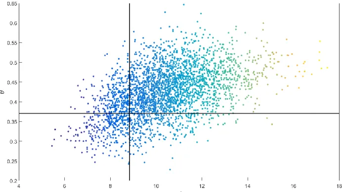
θ for a specific point in phase space describe the local behaviour of the segments of the trajectory that pass close to that point. A scatter plot of d versus θ is shown in Figure S1. A derivation of the two metrics, based upon (8, 19-21), is provided in the supporting information. d is closely linked to the
density of the trajectories (and hence to the local Lyapunov exponents), and provides a measure of the maximum divergence of the trajectories. In simple terms, a given atmospheric state with a low d is more likely to evolve in a similar way to all its neighbouring states than a case with high d. θ is the inverse of the average persistence time of trajectories around a given point, and it takes values in [0, 1]. Atmospheric states with a low θ are persistent and will therefore evolve—and diverge from neighbouring states—slowly. Both quantities are therefore closely linked to the predictability afforded by a given atmospheric state. Figure 1a provides an idealised illustration of the above for trajectories with low instantaneous dimension (blue trajectories) and high persistence (red trajectories).
We focus here on atmospheric configurations which have both low d and low θ, namely the states that should provide the maximum predictability of the trajectories’ forward paths. Specifically, we consider days where both d and θ are in the lowest 20 percentiles of their respective distributions. For the case of several consecutive days satisfying this condition, we select the first day in the series. The rationale behind this choice is to extract the maximum forward predictability from the metrics. This is also the most practical option for use in operational contexts. Say, for example, that we opted to select the local minimum of each threshold exceedance rather than the first day. For a series of several days continuously exceeding the threshold, the local minimum could only be determined at the end
4
of the series, while the initial exceedance can be spotted on the day it occurs.We do not simply select all days below the chosen percentile threshold because we wish to avoid double-counting when computing lagged composites. We term the selected events dynamical extremes. These account for ~4.4% of the time steps, or roughly 4 days every winter. The choice of the 20th percentile as threshold
is a compromise between the competing demands of selecting states that can be qualified as dynamical extremes and having a sufficiently large number of events. In fact, our aim is to identify a pathway for predictability which could be applied in an operational forecasting context. A result which, for example, were only to apply to 1 day every winter would have a limited value. Reasonable variations in this threshold were tested (22.5, 17.5, 12.5 percentiles) and were found not to qualitatively alter our conclusions (not shown).
The 2-m temperature extremes at each grid point are defined as all days exceeding the 10th and 90th
percentiles of the local distribution of deseasonalised anomalies. These are standard thresholds used in the literature (e.g. 22); repeating the analysis with the 5th and 95th percentiles (not shown) yields
qualitatively similar results. The anomalies are defined as departures from the long term daily average. For example, the climatological value for the 1st December is given by the mean of all 1st Decembers
in the dataset. We do not apply the same procedure as for the dynamical extremes to select temperature extremes because these are chosen based on their societal and economic impact rather than on considerations based on atmospheric configurations. It would indeed make little sense to only consider the first in a series of very cold or very warm winter days.
3. A Dynamical Systems Predictability Pathway
We now analyse the dynamical extremes as defined in Section 2 above. Figure 1b shows the compo-site 500 hPa geopotential height anomaly patterns for the selected events. These correspond to an anomaly dipole which is reminiscent of a positive NAO phase, albeit shifted to the east. In principle, two points with similar d and θ could represent very different flow configurations. We find this not be the case: the vast majority of the composite members agree on the sign of the anomalies suggesting that, at least for dynamical extremes, similar flow configurations generally correspond to similar re-gions in d – θ space. Coherent large-scale features are retained at positive lags, up to ~6-7 days fol-lowing the selected extremes (Figure S2 a, c, e, g), beyond which sign agreement is largely lost. Consistently with our interpretation of d and θ, the atmospheric patterns associated with the largest instantaneous dimension and lowest persistence diverge quickly at positive lags, and the geopotential height anomaly composites largely lose coherence by lag +3 (Figure S2 b, d, f, h).
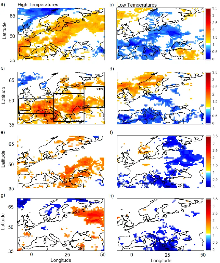
Climate or weather extremes are, by their very definition, rare. They should therefore generally be associated with similarly unusual large-scale atmospheric flow patterns (e.g. 23). While there is no guarantee that dynamical extremes correspond to weather extremes at a specific location, it is there-fore plausible to expect some correspondence between the two, at least at a continental scale. Figure 2 displays the changes in the frequency of two-metre temperature extremes associated with dynamical extremes, relative to the wintertime climatology. A value of 1 means that the frequency of temperature extremes is insensitive to the dynamical extremes; a value of 0 that there are no temperature extremes for the selected dynamical extremes; a value of 2 that there are twice as many temperature extremes as in the climatology. At lag 0 (2a, b) the dynamical extremes correspond to a higher frequency of warm extremes and a decreased frequency of cold extremes across large parts of Western, Continental and Northern Europe. At lag +4 days (2c, d) the pattern is similar, but now displays larger frequency changes for the warm extremes over the Mediterranean. The only regions showing an inverse pattern, with decreased warm occurrences and increased cold occurrences are northern and western Scandi-navia and the North Sea. By lag +6 days (2e, f) the largest changes in the temperature extremes have shifted eastwards and are now centred over Eastern and South-Eastern Europe. By day +8 (2g, h) there are two main regions of significant changes, with a heightened frequency of warm extremes over western Russia and a decrease in cold extremes over the Eastern Mediterranean. These changes
5
in extreme event frequency are largely consistent with the anomaly patterns shown in Figures 1b and S2. The cyclone-anticyclone dipole associated with the dynamical extremes, which displays a south-west to north-east tilt, draws warm subtropical air over most of Europe, with the exception of northern and western Scandinavia.
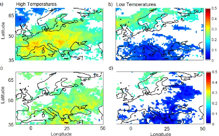
We next test the correspondence between dynamical extremes and the individual weather extremes at positive lags. Figure 3 displays the fraction of dynamical extremes which are followed within 2-4 days (3a, b) and 5-7 days (3c, d) by a temperature extreme. Note that if more than one temperature extreme falls within the lag interval for a single dynamical extreme, only one is counted. The dynam-ical extremes display significant hit rates for both warm and cold extremes across the whole continent up to 7 days. Hit rates for warm extremes locally exceed 40%, while hit rates for cold extremes reach below 4%. In other words, conditioning on a dynamical extreme significantly raises the chances of warm extremes and at the same time essentially excludes the possibility of cold extremes at a regional scale over several days. As expected, there is a good agreement between Figures 2 and 3, with the regions which show the largest positive changes in Figure 2, displaying high fractional matches in Figure 3.
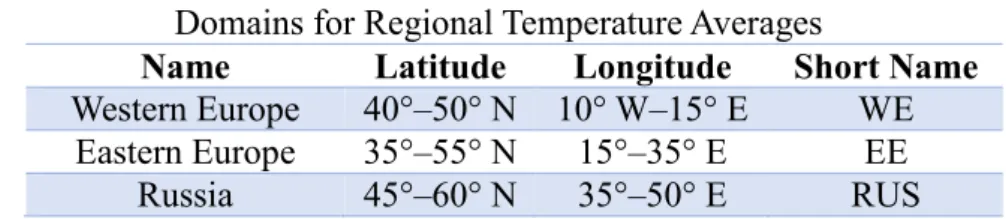
To further illuminate the predictability afforded by the dynamical extremes, we examine how the lagged distributions of regional temperature anomalies are modulated by the dynamical extremes. We focus on 3 broad domains selected to cover most of the European continent, marked by the black boxes in Figure 2c (see also Table S1). Figure 4 displays the cumulative distributions (CDFs) of land-only area-averaged temperature anomalies over these domains for the full wintertime climatology (blue) and conditional on the occurrence of a low d and θ episode (red), at lags of +2 to +4 days (4a, c, d) and +5 to +7 days (4b, d, f). In all domains, the dynamical extremes have major effects on the large-scale temperature anomalies. In Western Europe they correspond to significant increases in the 90th percentile, and associated changes in the amount of days exceeding them, at short positive lags
(4a). Over Eastern Europe a significant shift in both the 10th and 90th percentiles is seen at both lag
ranges (4c, d). Over Russia there is relatively little change at short lags, while at days +5 to +7 there is a marked shift in the 90th percentile of the distribution (4f). Finally, we note that all medians of the
distributions for dynamical extremes are statistically different from their climatological counterparts under a Wilcoxon rank sum test (24) at the 1% significance level. This is fully consistent with the reduction in cold extremes and increase in warm extremes shown in Figure 2.
4. Relation with the NAO
Temperatures extremes over Europe are often discussed in the context of the NAO (e.g. 22, 25). The two phases of the NAO are also the initialisation states that afford the best predictability in ensemble forecasts (13). Since the dynamical extremes should capture the atmospheric configurations offering the best predictability, it is not surprising that they resemble an NAO dipole. At the same time, it is important to highlight that these metrics provide complementary information to NAO-based analysis. We define a daily NAO index (NAOI) as the difference in average area-weighted 500 hPa height anomalies over the domains (70°W −10°W, 35°N−45°N) and (70°W −10°W, 55°N−70°N). This fol-lows the definition adopted by the National Oceanic and Atmospheric Administration’s Physical
Sci-ences Division of the Earth System Research Laboratory
(http://www.esrl.noaa.gov/psd/data/timeseries/daily/NAO/). The mean NAOI value for the dynam-ical extremes is -0.10 at lag -4, 0.22 at lag 0 and 0.15 at lag +4 days. One can further repeat the analysis presented in Figures 2 and 3 selecting NAO+ extremes with the same procedure used for dynamical extremes. We now use the 80th percentile as threshold, so as to obtain a similar number of events to the dynamical extremes (~4.1% instead of ~4.4%). Only ~5.1 % of the selected NAO+ extremes matches a dynamical extreme; similarly, roughly 25% of days above the NAO+ threshold match days below the dynamical extremes threshold. Consistently with this, the changes in the oc-currence of temperature extremes associated with the NAO display some important differences from
6
those seen for the dynamical extremes (cf. Figures 2 and S3). We further note that, while at lags 0 and 4 the NAO has a stronger impact on the temperature extremes than the dynamical extremes, the two become comparable around lag +6 and by lag +8 the dynamical extremes display a stronger regional footprint. This is consistent with our interpretation of dynamical extremes as the atmospheric states which give the best forward predictability as opposed to states which instantaneously corre-spond to the largest temperature anomalies.
5. Discussion and Conclusions
Simple instantaneous dynamical systems metrics can provide a robust indication of the atmospheric states providing the best forward predictability. Here, we apply this technique to the North Atlantic sector. A large part of the atmospheric variability, and predictability, in this region is associated with the NAO. It is therefore reassuring that the atmospheric configuration we obtain from our dynamical system analysis resembles an NAO dipole. At the same time the high predictability days we select, termed dynamical extremes, do not systematically match NAO extremes. We therefore conclude that a dynamical systems approach provides complementary information to an NAO-based analysis. Our dynamical systems perspective further provides a definition of extreme event which differs from the standard statistical view formalized by Pickands and Pareto (26), where extremes are large or small events with respect to a certain local observable. For complex fields, the dynamical systems approach can capture the crucial link between large-scale non-static phenomena and local effects. In the context of this study, a more traditional definition of a “geopotential extreme” could be for exam-ple to compute a Euclidean distance of daily fields from the long-term mean field and define extremes as days in the top and bottom percentiles of this distribution. However, if this approach is used, se-lecting a similar number of occurrences as for the dynamical extremes, the link between the geopo-tential extremes and the predictability of temperature extremes over Europe is weak (see Figure S4 and Text S2).
On the contrary, the dynamical extremes provide a strong predictability pathway for wintertime tem-perature extremes over the European continent at timescales of up to a week. This is underscored by the significant modulation of regional temperature extremes associated with dynamical extremes. In this respect, we highlight that a forecast of a decreased probability of an extreme can be as valuable societally and economically as the forecast of an increased probability of an extreme. The link be-tween dynamical extremes and cold spells is therefore important, even though the extremes system-atically correspond to decreased occurrences of low temperatures. An additional analysis considering states with low d and low θ separately (not shown) highlights that, in general, persistence provides a better indication of predictability than instantaneous dimension. This suggests that the rapidity with which nearby trajectories diverge from a neighbourhood is typically, but not always, more relevant than their maximum spread while doing so. The insights provided by the two dynamical systems metrics can complement the information issued by deterministic and ensemble forecasts, which are currently used by many national emergency response services (e.g. 27). The same metrics could be further used as diagnostic tools to evaluate current operational ensemble forecast products.
The analysis presented in this study points to several pathways for future research. Keeping the focus on the North Atlantic, it is necessary to verify whether the low d and θ states which do not agree with the sign of the geopotential height anomaly composite actually correspond to a separate cluster in phase space relative to the ones that do. This would allow for a more accurate quantification of the predictability afforded by the dynamical extremes. More generally, the methodology we adopt could be applied to domains which, unlike the North Atlantic, might not have a clearly recognisable domi-nant mode of atmospheric variability. An obvious caveat is that there is no guarantee that dynamical extremes will be associated with a given class of weather extremes over a specific geographical do-main, meaning that this technique might not always be appropriate for targeted regional studies. At
7
the same time, we note that the dynamical systems metrics provide a general information about at-mospheric trajectories, meaning that their use can be extended to predictability problems unrelated to extreme events. On the more technical side, it will be necessary to provide a robust quantification of the typical predictability horizon afforded by the dynamical systems perspective, by performing a comprehensive analysis on the variability of d and θ and their co-variance. It would be further inter-esting to investigate the link between the predictability limit in a chaotic atmosphere as formulated by Lorenz and the magnitude of the extremes in d and θ.
Acknowledgements
During this work, G. Messori has been funded by a grant of the Department of Meteorology of Stock-holm University. ERA-Interim reanalysis data are freely available from the ECMWF at http://apps.ecmwf.int/datasets/.
References
1. Lorenz, E. N. (1980), Attractor sets and quasi-geostrophic equilibrium . J. Atmos. Sci. 37, 1685– 1699.
2. Grassberger P (1986) Do climatic attractors exist? Nature 323:609-612.
3. Lorenz EN (1991) Dimension of weather and climate attractors. Nature 353:241-244.
4. Kunkel, K. E., Pielke Jr, R. A., & Changnon, S. A. (1999). Temporal fluctuations in weather and climate extremes that cause economic and human health impacts: A review. Bull. Am. Meteorol.
Soc., 80(6), 1077.
5. Gasparrini A, Guo Y, Hashizume M, Lavigne E, Zanobetti A, Schwartz J, …, Leone M. (2015), Mortality risk attributable to high and low ambient temperature: a multicountry observational study. The Lancet, 386(9991), 369–375.
6. Herring, S. C., Hoerling, M. P., Kossin, J. P., Peterson, T. C., & Stott, P. A. (2015). Explaining extreme events of 2014 from a climate perspective. Bull. Am. Meteorol. Soc., 96(12), S1-S172. 7. Vautard, R. & Ghil, M. (1989), Singular spectrum analysis in nonlinear dynamics, with
applica-tions to paleoclimatic time series . Physica D 35, 395–424.
8. Lucarini, V. et al. Extremes and Recurrence in Dynamical Systems. Pure and Applied Mathemat-ics: A Wiley Series of Texts, Monographs and Tracts (Wiley, 2016).
9. Analitis, A., Katsouyanni, K., Biggeri, A., Baccini, M., Forsberg, B., Bisanti, L. ... & Hojs, A. (2008). Effects of cold weather on mortality: results from 15 European cities within the PHEWE project. American journal of epidemiology, 168(12), 1397-1408.
10. Gooding, M. J., Ellis, R. H., Shewry, P. R., & Schofield, J. D. (2003). Effects of restricted water availability and increased temperature on the grain filling, drying and quality of winter wheat.
Journal of Cereal Science, 37(3), 295-309.
11. Beniston, M. (2005). Warm winter spells in the Swiss Alps: Strong heat waves in a cold season? A study focusing on climate observations at the Saentis high mountain site. Geophys. Res. Lett.,
8
12. Johansson, Å. (2007). Prediction skill of the NAO and PNA from daily to seasonal time scales.
J.Clim., 20(10), 1957-1975.
13. Ferranti, L., Corti, S. and Janousek, M. (2015), Flow-dependent verification of the ECMWF en-semble over the Euro-Atlantic sector. Q.J.R. Meteorol. Soc., 141: 916–924. doi:10.1002/qj.2411 14. Dee, D. P., Uppala, S. M., Simmons, A. J., Berrisford, P., Poli, P., Kobayashi, S., ... & Bechtold, P. (2011). The ERA‐Interim reanalysis: Configuration and performance of the data assimilation system. Q.J.R. Meteorol. Soc., 137(656), 553-597.
15. Faranda D, Messori G and Yiou P. (2017) Dynamical proxies of North Atlantic predictability and extremes. Sci. Rep., in press, DOI: 10.1038/srep41278.
16. Baldwin, M. P., & Dunkerton, T. J. (2001). Stratospheric harbingers of anomalous weather re-gimes. Science, 294(5542), 581-584.
17. Michelangeli, P. A., Vautard, R., & Legras, B. (1995). Weather regimes: Recurrence and quasi stationarity. J. Atmos. Sci., 52(8), 1237-1256.
18. Davini, P., Cagnazzo, C., Gualdi, S., & Navarra, A. (2012). Bidimensional diagnostics, variability, and trends of Northern Hemisphere blocking. J. Clim., 25(19), 6496-6509.
19. Freitas, A. C. M., Freitas, J. M. & Todd, M. (2010), Hitting time statistics and extreme value theory. Probab. Theory Rel. 147, 675–710.
20. Faranda D, Lucarini V, Turchetti G, Vaienti S (2011) Numerical convergence of the block-max-ima approach to the generalized extreme value distribution. J. Stat. Phys. 145:1156-1180.
21. Lucarini, V., Faranda, D. & Wouters, J. (2012), Universal behaviour of extreme value statistics for selected observables of dynamical systems. J. Stat. Phys. 147, 63–73.
22. Yiou, P., and M. Nogaj (2004). Extreme climatic events and weather regimes over the North At-lantic: When and where? Geophys. Res. Lett., 31, L07202.
23. Grotjahn, R., Black, R., Leung, R., Wehner, M. F., Barlow, M., Bosilovich, M., ... & Lee, Y. Y. (2016). North American extreme temperature events and related large scale meteorological pat-terns: a review of statistical methods, dynamics, modeling, and trends. Clim. Dyn., 46(3-4), 1151-1184.
24. Mann, H. B., Whitney, D. R. (1947). On a Test of Whether one of Two Random Variables is Stochastically Larger than the Other. Annals Mat. Stat., 18 (1): 50–60. doi:10.1214/aoms/1177730491.
25. Cassou, C. (2008). Intraseasonal interaction between the Madden–Julian oscillation and the North Atlantic oscillation. Nature, 455(7212), 523-527.
26. Pickands III, J. (1975). Statistical inference using extreme order statistics. Ann. Stat., 119-131. 27. Sene, K. (2008). Flood warning, forecasting and emergency response. Springer Science &
9
Figure Captions
Figure 1. a) Example of trajectories evolving from neighbourhoods (marked by the green spheres)
with low instantaneous dimension (blue trajectories) and high persistence (red trajectories) in an ide-alised 3-dimensional phase space. The low dimension implies that the maximum divergence of the blue trajectories is small, but gives no information on how rapidly they leave the neighbourhood. The high persistence implies that the trajectories are slow in leaving the neighbourhood, but gives no information on their maximum divergence. Composite 500 hPa geopotential height anomalies (m) for days corresponding to low d and θ (b). The grey shading marks regions where more than 60% of the members of the composite agree on the sign of the anomalies. The chance of this happening randomly is well below 1%.
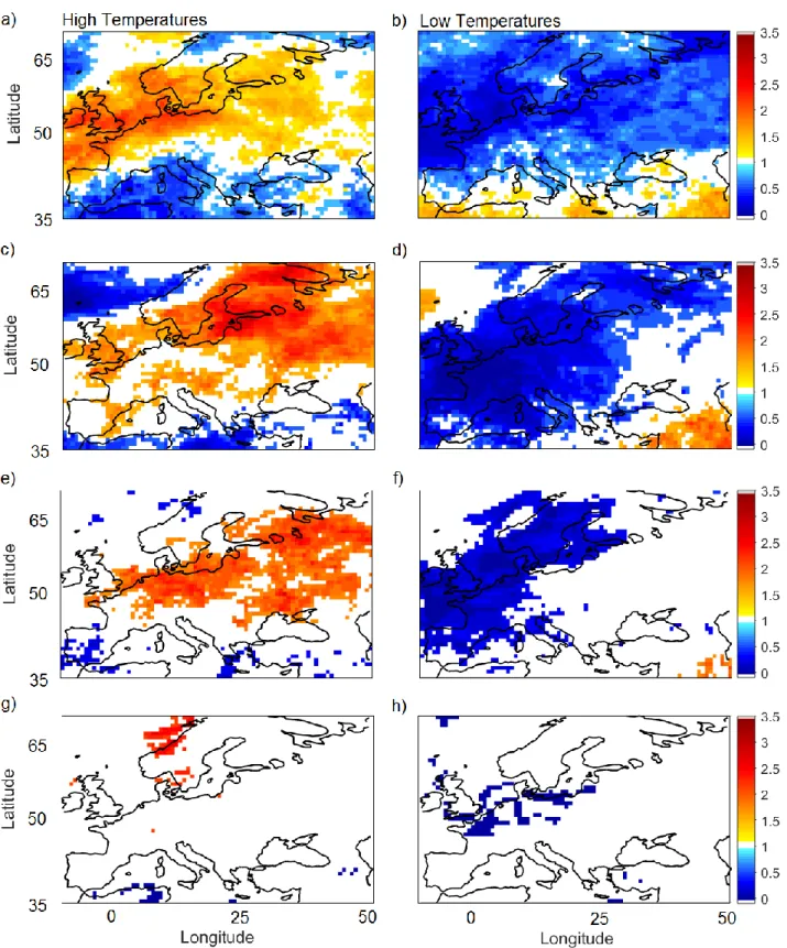
Figure 2. Fractional changes in the frequency of wintertime hot (a, c, e, g) and cold (b, d, f, h) surface
temperature extremes conditional on low instantaneous dimension and high persistence events rela-tive to the climatology, at (a, b) lag 0; (c, d) lag +4, (e, f) lag +6 and (g, h) lag +8 days. The black boxes in panel (c) mark the domains used in Figure 4 (see also Table S1). Only values exceeding the 5% significance level, computed using a Monte Carlo procedure with 1000 random samples are shown.
Figure 3. Fraction of low instantaneous dimension and high persistence extremes associated with hot (a, c) and cold (b, d) wintertime surface temperature extremes at a given location, at (a) lags +2 to +4 and (b) lags +5 to +7 days. Only values exceeding the 5% significance level, computed using a Monte Carlo procedure with 1000 random samples (see Methods), are shown.
Figure 4. Empirical cumulative distributions of land-only area-averaged 2-metre temperature
anom-alies (K). The blue curves correspond to the wintertime climatology; the red are conditional on the occurrence of a dynamical extreme 2 to 4 days (a, c, e) and 5 to 7 days (b, d, f) before. The dashed vertical lines mark the climatological 10th and 90th percentiles. The continuous vertical lines mark the medians of the two distributions. The blue crosses mark the statistical significance for the shift in the percentiles (horizontal bars) and the change in the number of events above/below the climatological percentiles (vertical bars). The edges of the bars correspond to the 5% significance level, computed using a Monte Carlo procedure with 1000 random samples (see Methods). See Table S1 for the do-main boundaries.
Figure S1. Scatter plot of d versus θ for 500 hPa geopotential height anomalies. The black lines mark
the thresholds used to define the dynamical extremes (see Methods).
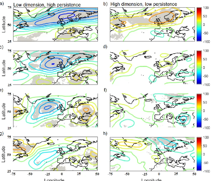
Figure S2. Composite 500 hPa geopotential height anomalies (m) for days corresponding to low
instantaneous dimension and high persistence (a, c, d, g) and days corresponding to high instantane-ous dimension and low persistence (b, d, f, h) at lags of (a, b) 0, (c, d) +4, (e, f) +6 and (g, h) +8 days. The grey contours mark regions where more than 60% of the members of the composite agree on the sign of the anomalies. The chance of this happening randomly is below 1% (see Methods).
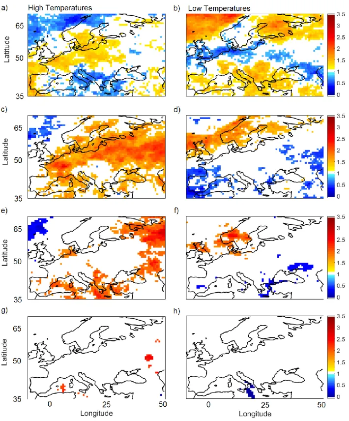
Figure S3. Fractional changes in the frequency of wintertime hot (a, c, e, g) and cold (b, d, f, h)
surface temperature extremes conditional on high NAO events relative to the climatology, at (a, b) lag 0; (c, d) lag +4, (e, f) lag +6 and (g, h) lag +8 days. Only values exceeding the 5% significance level, computed using a Monte Carlo procedure with 1000 random samples are shown.
Figure S4. Fractional changes in the frequency of wintertime hot (a, c, e, g) and cold (b, d, f, h)
surface temperature extremes conditional on geopotential extremes as defined in Text S2, at (a, b) lag 0; (c, d) lag +4, (e, f) lag +6 and (g, h) lag +8 days. Only values exceeding the 5% significance level,
10
11
Figures
Figure 1. a) Example of trajectories evolving from neighbourhoods (marked by the green spheres)
with low instantaneous dimension (blue trajectories) and high persistence (red trajectories) in an ide-alised 3-dimensional phase space. The low dimension implies that the maximum divergence of the blue trajectories is small, but gives no information on how rapidly they leave the neighbourhood. The high persistence implies that the trajectories are slow in leaving the neighbourhood, but gives no information on their maximum divergence. Composite 500 hPa geopotential height anomalies (m) for days corresponding to low d and θ (b). The grey shading marks regions where more than 60% of the members of the composite agree on the sign of the anomalies. The chance of this happening randomly is well below 1%.
12
Figure 2. Fractional changes in the frequency of wintertime hot (a, c, e, g) and cold (b, d, f, h) surface
temperature extremes conditional on low instantaneous dimension and high persistence events rela-tive to the climatology, at (a, b) lag 0; (c, d) lag +4, (e, f) lag +6 and (g, h) lag +8 days. The black boxes in panel (c) mark the domains used in Figure 4 (see also Table S1). Only values exceeding the 5% significance level, computed using a Monte Carlo procedure with 1000 random samples are shown.
13
Figure 3. Fraction of low instantaneous dimension and high persistence extremes associated with hot (a, c) and cold (b, d) wintertime surface temperature extremes at a given location, at (a) lags +2 to +4 and (b) lags +5 to +7 days. Only values exceeding the 5% significance level, computed using a Monte Carlo procedure with 1000 random samples (see Methods), are shown.
14
Figure 4. Empirical cumulative distributions of land-only area-averaged 2-metre temperature
anom-alies (K). The blue curves correspond to the wintertime climatology; the red are conditional on the occurrence of a dynamical extreme 2 to 4 days (a, c, e) and 5 to 7 days (b, d, f) before. The dashed vertical lines mark the climatological 10th and 90th percentiles. The continuous vertical lines mark the
medians of the two distributions. The blue crosses mark the statistical significance for the shift in the percentiles (horizontal bars) and the change in the number of events above/below the climatological percentiles (vertical bars). The edges of the bars correspond to the 5% significance level, computed using a Monte Carlo procedure with 1000 random samples (see Methods). See Table S1 for the do-main boundaries.
15
Supporting Information for
A Dynamical Systems Approach to studying
Mid-Latitude Weather Extremes
Gabriele Messori1*, Rodrigo Caballero1, Davide Faranda2
1Department of Meteorology and Bolin Centre for Climate Research, Stockholm University, 114 18, Stockholm, Sweden. 2Laboratoire des Sciences du Climat et de l’Environnement, LSCE/IPSL, CEA-CNRS-UVSQ, Université Paris-Saclay,
F-91191, Gif-sur-Yvette, France.
* Correspondence to Gabriele Messori: Department of Meteorology, Svante Arrhenius Väg 16c, 114 18, Stockholm, Sweden; e-mail: [email protected]; tel.: 0046 81610812.
Contents of this file
Texts S1 and S2 Table S1
Figures S1 to S4
Introduction
The present Supporting Information includes a brief description of how instantaneous dimension and persistence are computed (Text S1); a discussion of an alternative definition for atmospheric extremes based on Euclidean distance; a definition of geographical domains used for Figure 4 (Table S1); a scatterplot of instantaneous dimension versus persistence (Figure S1); an overview of the geopotential height anomalies associated to atmospheric states with high and low instantaneous dimension and persistence (Figure S2) and the equivalent of Figure 2 computed based on extreme NAO+ events (Figure S3) and maximum Euclidean distance of geopotential maps from the climatology (Figure S4) rather than dynamical extremes.
Text S1
In order to compute the instantaneous dimension and persistence of the geopotential height field, we treat each timestep in the dataset as a point along a single trajectory ξ(t). At each time t, we define the instantaneous properties of the state ξ. The properties change with time, and are therefore instantane-ous. We further note that states which are close in phase space will have similar instantaneous prop-erties, although the converse is not necessarily true.
To compute our two metrics for a point ξ(t1), we consider theprobability P associated with the
trajec-tory returning within a radius r of said point. We define the distance between ξ(t1) and all other
ob-servations along the trajectory as:
𝑔(𝜉(𝑡)) = −log (𝜍(𝜉(𝑡), 𝜉(𝑡1)))
Where 𝜍 is a distance function (in our case the euclidean distance between the geopotential height maps) and the logarithm increases the discrimination of small separations. We then apply the Freitas-Freitas-Todd theorem (19, 21) to express this probability as a generalised Pareto distribution:
𝑃 (𝑔(𝜉(𝑡)) > 𝑞, 𝜉(𝑡1)) ≃ 𝑒(
𝑥+𝜇(𝜉(𝑡1))
𝜎(𝜉(𝑡1)) )
16 𝑑(𝜉(𝑡1)) =
1 𝜎(𝜉(𝑡1))
The threshold q in (2) above can be expressed as: 𝑞 = 𝑒−𝑟
Imposing that 𝑔(𝜉(𝑡)) > 𝑞 is therefore equivalent to the condition that the trajectory returns within a radius r of the point ξ(t1). q can therefore simply be set as a percentile of 𝑔(𝜉(𝑡)).
In the present paper we use q = 0.98. Its appropriateness is determined by ensuring that more than 95% of the observations along our trajectory satisfy the Anderson-Darling test at the 0.05 significance level.
We can further compute a measure of the residence time of ξ(t) within a radius r of ξ(t1), by adding
an extremal index parameter θ to (2):
𝑃 (𝑔(𝜉(𝑡)) > 𝑞, 𝜉(𝑡1)) ≃ 𝑒(𝜃(
𝑥+𝜇(𝜉(𝑡1))
𝜎(𝜉(𝑡1)) ))
θ-1 is then the mean residence time of the trajectory within the neighbourhood defined by r.
By applying the above procedure, we therefore obtain a value of d and θ for every timestep in our dataset.
The only requirement of our methodology is that ξ(t) must be sampled from an underlying ergodic system. For further theoretical details, the reader is referred to (8, 15).
Text S2
As discussed in Section 5 in the main paper, we define geopotential extremes by first computing the Euclidean distance of daily 500 hPa geopotential height maps from the long-term winter climatology. We then apply exactly the same procedure as for the dynamical extremes (except that we now select events above the 80th percentile). This yields a similar number of events (~4.6% of winter days instead of ~4.4%). Finally, we produce maps of the fractional changes in the frequency of wintertime hot and cold surface temperature extremes over Europe (Figure S4), which can be compared to those shown in Figures 2 and S3.
The geopotential extremes show a strong footprint on the European temperature extremes at short lead times (0-4 days), but have a weak link with the temperatures beyond this timescale. By lag +8 the signal has completely disappeared. This is fully consistent with the physical interpretation of the geopotential extremes, which represent unusual instantaneous atmospheric configurations but a priori contain no information on the evolution of these states.
17
Domains for Regional Temperature Averages
Name Latitude Longitude Short Name
Western Europe 40°–50° N 10° W–15° E WE Eastern Europe 35°–55° N 15°–35° E EE
Russia 45°–60° N 35°–50° E RUS
18
Figure S1. Scatter plot of d versus θ for 500 hPa geopotential height anomalies. The black lines mark
19
Figure S2. Composite 500 hPa geopotential height anomalies (m) for days corresponding to low
instantaneous dimension and high persistence (a, c, d, g) and days corresponding to high instantane-ous dimension and low persistence (b, d, f, h) at lags of (a, b) 0, (c, d) +4, (e, f) +6 and (g, h) +8 days. The grey contours mark regions where more than 60% of the members of the composite agree on the sign of the anomalies. The chance of this happening randomly is below 1% (see Methods).
20
Figure S3. Fractional changes in the frequency of wintertime hot (a, c, e, g) and cold (b, d, f, h)
surface temperature extremes conditional on high NAO events relative to the climatology, at (a, b) lag 0; (c, d) lag +4, (e, f) lag +6 and (g, h) lag +8 days. Only values exceeding the 5% significance level, computed using a Monte Carlo procedure with 1000 random samples are shown.
21
Figure S4. Fractional changes in the frequency of wintertime hot (a, c, e, g) and cold (b, d, f, h)
surface temperature extremes conditional on geopotential extremes as defined in Text S2, at (a, b) lag 0; (c, d) lag +4, (e, f) lag +6 and (g, h) lag +8 days. Only values exceeding the 5% significance level, computed using a Monte Carlo procedure with 1000 random samples are shown.