HAL Id: halshs-01254475
https://halshs.archives-ouvertes.fr/halshs-01254475
Preprint submitted on 12 Jan 2016
HAL is a multi-disciplinary open access
archive for the deposit and dissemination of sci-entific research documents, whether they are pub-lished or not. The documents may come from teaching and research institutions in France or abroad, or from public or private research centers.
L’archive ouverte pluridisciplinaire HAL, est destinée au dépôt et à la diffusion de documents scientifiques de niveau recherche, publiés ou non, émanant des établissements d’enseignement et de recherche français ou étrangers, des laboratoires publics ou privés.
Bank output calculation in the case of France: what do
new methods tell about the financial intermediation
services in the aftermath of the crisis?
Groslambert Bertrand, Raphaël Chiappini, Olivier Bruno
To cite this version:
Groslambert Bertrand, Raphaël Chiappini, Olivier Bruno. Bank output calculation in the case of France: what do new methods tell about the financial intermediation services in the aftermath of the crisis?. 2016. �halshs-01254475�
Bank Output CalCulatiOn in the Case
Of franCe: What DO neW MethODs tell
aBOut the finanCial interMeDiatiOn
serviCes in the afterMath Of the
Crisis?
Documents de travail GREDEG
GREDEG Working Papers Series
Bertrand Groslambert
Raphaël Chiappini
Olivier Bruno
GREDEG WP No. 2015-32
http://www.gredeg.cnrs.fr/working-papers.html
Les opinions exprimées dans la série des Documents de travail GREDEG sont celles des auteurs et ne reflèlent pas nécessairement celles de l’institution. Les documents n’ont pas été soumis à un rapport formel et sont donc inclus dans cette série pour obtenir des commentaires et encourager la discussion. Les droits sur les documents appartiennent aux auteurs.
The views expressed in the GREDEG Working Paper Series are those of the author(s) and do not necessarily reflect those of the institution. The Working Papers have not undergone formal review and approval. Such papers are included in this series to elicit feedback and to encourage debate. Copyright belongs to the author(s).
1
Bank output calculation in the case of France: what do
new methods tell about the financial intermediation
services in the aftermath of the crisis?
Bertrand GROSLAMBERT*, Raphaël CHIAPPINI#, Olivier BRUNOǂGREDEG Working Paper No. 2015-32
Abstract: Since the onset of financial crisis, the System of National Accounts method for
measuring the value added in the banking sector has become subject to criticism. Some authors argue that the value added by banks should be the residual net interest income after subtracting the required term and risk premiums on loans and deposits. For the first time, we apply this method to evaluate bank output for France for the period 2003 to 2012. First, we show that on average, using the traditional method, bank output is overestimated by between 31% and 74%. This overestimation is especially pronounced in times of financial stress. Second, we establish that the proposed new method is robust to the choice of various reference rates. Third, we find negative FISIM (Financial Intermediation Services Indirectly Measured) on deposits from 2009. Finally, we check the existence of a single or multiple structural unknown breaks in the long run relationship between retail interest rates and driving market reference rates. We find existence of break dates that are coincident with negative FISIM on deposits. We explain this result by a change in banking behavior that may result from the new banking regulation on liquidity and from banks' adaptation to "near" zero interest rate policy.
Keywords: FISIM, interest rate pass-through, structural break JEL: E43, G21
* SKEMA Business School – Université de Lille, ECCCS Research Center, bertrand.groslambert@skema.edu
# Université Nice Sophia Antipolis, GREDEG-CNRS, raphaël.chiappini@gredeg.cnrs.fr
ǂ Corresponding author. Université Nice Sophia Antipolis, GREDEG-CNRS, SKEMA Business School and
2
1. Introduction
Measuring the output of the banking system is challenging since many of the services provided by banks are not charged directly to customers. The System of National Accounts (SNA 1993) has developed a methodology based on a "single reference" rate. Deposits provide banks with funds at below the rates they would pay were they obtaining finance in the market. Symmetrically, banks lend at higher rates than they would receive if they chose to invest those funds in the market. The difference between the rates of interest payable and receivable on loans and deposits is used to measure bank output.
The problem with this method relies on the "single reference" rate defined as the average rate at which banks lend money to each other, and which is used to measure the cost of funds for all types of activities (loans and deposits). Consequently, it does not tackle the difference in maturity and risk among the various types of loans and deposits made by banks. It means that compensations for term and risk premiums are treated as productive services offered by the bank. Authors such as Wang (2003), Basu, Inklaar and Wang (2011), Colangelo and Inklaar (2012), Wang and Basu (2011) consider that the remuneration related to risk-taking and term premiums does not fall within the productive activities of banks since these risks ultimately are supported by the providers of bank capital. Consequently, only the portion of interest income related to monitoring and controlling borrowers should be recorded. Colangelo and Inklaar (2012) propose a new method to compute bank output, using interest rate pass-through in order to choose the interest rate exclusive of term and risk premiums.1
However, the relevance of this new method is still open to question. The main problem lies in the reliability and stability of their results. The choice of a reference rate using interest rate pass-through is very sensitive to time period and to the country considered. Sorensen and Werner (2006) show there is a large heterogeneity in the pass-through of market to bank rates among euro area countries. Furthermore, as suggested by De Bondt (2005), there are many factors that can influence the interest rate pass-through. Thus, both the financial and the euro area debt crises could have affected the pass-through of retail bank interest rates, and thus, the calculation of bank output.
In this paper, we propose to apply the new method to French data for the period 2003 to 2012. We chose France since, unlike the USA for example, it had experienced a declining share of finance in its GDP since the mid-1980s (Philippon and Reshef, 2013). Also, it allows us to test the reproducibility of the new method for a specific country, its robustness to the choice of reference rate, and its sensitivity to the financial crisis.
Our results are the following. First, we find that the value added of French banks computed using the traditional method is overestimated in average by 31-74% for the period 2003 – 2012. This outcome is in line with previous studies on the U.S. and the Eurozone and we establish that this result is robust to the choice of various reference market rates retained using the pass-through methodology. However, we show that there is a high degree of heterogeneity in FISIM measurement from year to year. In particular, we find that the results obtained using the traditional and the new method are widely divergent during times of financial stress. Second, we find negative FISIM on deposits from 2009 in France. In order to explain this result, we search for a structural break in the interest pass-through and we find that there is a change in
1 The new method shows that bank output is overestimated by the traditional method, respectively by 21% for the USA and on average by 24% to 40% for the Eurozone (Basu, Inklaar and Wang, 2011; Colangelo and Inklaar, 2012).
3
bank behavior around 2007 and 2009. We provide two complementary explanations to this result. The first one is linked to the "near" zero interest-rate policy conducted by the European central bank. As margin behavior is less important on deposits than on loans, banks decide not to pass all the decrease in interest rate on deposit rate. The second explanation is linked with the new regulatory requirement on liquidity that will be imposed by Basel III. It means that deposits are now a vital stable resource of liquidity for banks that seems to be ready to pay for it.
The rest of the paper is organized as follow. Section 2 presents the analytical framework that found the new measurement of FISIM whereas section 3 describes our database and methodology. Our main results are exposed in section 4. Section 5 concludes.
2. The analytical framework: from the current to the new methodology for computing Financial Intermediation Services Indirectly Measured (FISIM)
Debates about how estimating the level of bank production has existed as early as 1952 when the very first standardized System of National Accounts was implemented (OECD, 1998). The 1968 SNA and then the 1993 SNA tried to improve the method but have been inconclusive.2 First, as noted in the 2008 System of National Accounts (UN, 2008), “the way in which financial institutions charge for the services they provide is not always as evident as the way in which charges are made for most goods and services.” Banks do not explicitly charge for some of their services. Instead, a significant part of their outcome is implicitly derived from the interest rate margin between deposits and loans. The second challenge is to disentangle the part of the spread that is due to the cost of funds and the one that corresponds to the services offered by the bank.
Circumventing these difficulties for computing the amount of FISIM, the System of National Accounts (SNA 1993, ESA 1995 and SNA 2008), suggests using an arbitrary reference rate, such as the interbank rate. Under this rule of thumb, one can calculate FISIM on deposits d
Y and FISIM on loans l
Y . FISIM on deposits come from the difference between the reference rate f
r and the rate actually paid to depositors d
r times the deposit amounts. FISIM on loans are given by the difference between the rate paid to banks by borrowers l
r and the reference rate f
r times the loan amount. We obtain
(
)
deposits
loans (
)
d f d l l fY
r
r
Y
r
r
=
×
−
=
×
−
Adding explicitly charged services to the FISIM and deducting intermediate consumption gives the value added of the banking industry.
FISIM
+ Explicitly charged services – Intermediate consumption = Value added
4
This method has been adopted since 1993. However, the 2008 financial crisis caused great volatility in the FISIM output and has raised a series of questions about its relevance and reliability. Results generated during this period have been found implausible (Davies, 2010). In some occasions, negative FISIM occurred, whereas in other cases, FISIM output grew at surprisingly high rate. The reason is that, paradoxically in times of rising risk, when banks increase their rates to cover against possible default, the current method automatically generates additional output for banks. That’s why, in the wake of the 2008 crisis, the widening of interest rate spreads has mechanically inflated the FISIM, increasing significantly the contribution of the banking sector to GDP (Mink, 2008). Referring to the Japanese economic situation, Sakuma (2013) has made the same observation, especially during the years 2002-2004.3 In order to address these questions, two working groups were created in 2010.4 Their final report was published in May 2013 (ISWGNA, 2013). However, they have not been able to reach a consensus on a method for calculating FISIM (Ahmad, 2013).
Mink (2010), Diewert et al. (2012) or Zieschang (2013) review the different approaches. The main issue opposing researchers is whether the remuneration related to the management of liquidity risk and the compensation related to the risk of default must be recorded in the production account. As Schreyer (2009) or Zieschang (2013) explain, the key question is who bears the risk and consequently how should the financial risk management activities be dealt with. Answering this question determines the choice of the reference rate used for calculating the FISIM.
Some authors such as Ruggles (1983), argue that banks’ role is to directly provide finance to borrowers as opposed to those who consider banks as providers of financial services. For these researchers, banks bear the risk themselves and their output should include the compensation for taking that risk. Their margin must include a risk premium and therefore the reference rate should be a risk-free rate as explained in Fixler et al. (2010). For them, the reference rate represents the opportunity cost of deposits, which is the return that the bank would get if it was invested in assets liquid and stable enough for allowing fund withdrawal at any time. Meanwhile, the reference rate also represents the opportunity cost of the bank’s loans. It is the return that the bank foregoes by lending to its customers rather than investing into liquid assets with no credit risk. This approach corresponds to the existing System of National Accounts (SNA 1993, ESA 1995, SNA 2008). It is currently implemented in the European Union and in the United States, who respectively use an interbank rate and a government risk-free rate as reference rate. Alternative ways to compute the reference rate exist. The Australian Bureau of Statistics uses a midpoint of weighted average borrowing and lending rates (Cullen, 2011). Others such as Diewert, Fixler and Zieschang (2012), or Zieschang (2013) suggest taking the cost of funds or the cost raising financial capital as reference rate. All these methods have a common characteristic: they rely on a single reference rate which means that they incorporate a certain amount of term and risk premium in the calculation of the FISIM.
Another stream of research made of Wang (2003), Wang, Basu and Fernald (2009), Basu, Inklaar and Wang (2011), Colangelo and Inklaar (2012), Inklaar and Wang (2013) and Wang and Basu (2013) considers that the output of banks does not depend on the amount of risk they
3 Sakuma (2013) reviews the various methods that have been implemented to evaluate the production of the financial sector since 1953. According to the author, the economic situation in Japan and its impact on the estimation of the Japanese banking production revealed well before 2008, the shortcomings of the method used by the System of National Accounts.
4 These are the "ISWGNA Task Force on FISIM" for the United Nations and the "European task Force on FISIM" for the European Union.
5
take. Those researchers, called the Wang camp by Diewert (2013), think that the compensation for taking risk must be removed from the calculation of bank production. For these authors, as for Schreyer and Stauffer (2011), banks are simply producers of financial services, whose role and purpose is to reduce information asymmetry between investors and borrowers through controlling and monitoring. For Wang (2003), the remuneration related to risk-taking does not fall within the productive activities of banks since risk is ultimately supported by providers of capital. This remuneration should be recorded as an allocation of income account as the System of National Accounts recommends for any property income. Only the portion of interest income related to the monitoring and controlling of borrowers should be recorded in the FISIM. To illustrate this point and highlight the shortcomings of the current method, Wang et al. (2009) propose to consider the hypothetical case of a "bank that does nothing". This bank has the only function to serve as a pipeline between savers and borrowers, without performing any controlling or monitoring. This bank would finance on short-term market and would simply record loans in its balance sheet. It would strictly do nothing, providing no service and not creating any wealth. If the economic cycle is favorable, such a bank could generate substantial profits by pocketing the term premium and the credit risk premium. Under the current System of National Accounts, this bank would also generate some value added, even though it has no activity at all.
For Wang (2003), credit risk is not borne by banks but rather by the providers of capital. The activity of financial intermediaries only consists in delivering financial services. Consequently, their value added must not comprise any risk premium. Reference rates must be based on the cost of funds and exclude those premia. Therefore, Basu, Fernald, Inklaar and Wang (BFIW)5 suggest, for each type of loan, the interest rate of a market debt security with the same risk profile and maturity but with no service attached in order to calculate bank output generated by lending activities. This removes the credit risk premium as well as any term premium from the calculation of FISIM on loans. Regarding depositor services and assuming that deposits are all insured, BFIW recommend using different risk-free rates according to the maturity of each type of deposits. In contrast to loan services, depositor services include a term premium and the reference rate should be chosen accordingly. In that respect, Colangelo and Inklaar (2012) note that the current European national accounts system underestimates the value of depositor services since the reference rate is only a short term maturity, which removes the term premium from the calculation of FISIM on deposits.
Figure 1 summarizes the differences between the usual SNA, and the BFIW methodology. We assume that:
l
r , the average interest rate received on loans
m
r , the expected rate of return required on market securities with the same systematic risk characteristics as the loans
'
f
r , the risk-free interest rate on government securities
f
r , the risk-free rate on money market
d
r , the average interest rate paid on deposits
l
Y , the nominal output of bank services to borrowers
d
Y , the nominal output of bank services to depositors
5 See Wang, Basu and Fernald (2009), Inklaar and Wang (2013), Basu, Inklaar and Wang (2011), Wang and Basu (2011), and Colangelo and Inklaar (2012).
6
Figure 1: The calculation of banks FISIM
In the paper, we adopt the method proposed by Colangelo and Inklaar (2012) and compute FISIM for France excluding term and risk premium from 2003 to 2012.
3. Data and methodology
This part presents the methodology for computing FISIM under the alternative approach and the data used for this calculus.
3.1. Data description
We exploit mainly the Webstat Banque de France database augmented by the European Central Bank (ECB) Statistical Data Warehouse for series on loans and deposits.6 Interest rates on market debt security come from the ECB database, Bloomberg, Markit Iboxx and Merrill Lynch Bank of America. In the case of France, the Webstat Banque de France statistical series do not exactly correspond to the ECB Statistical Data Warehouse series used in Colangelo and Inklaar (2012). Although the ECB website provides data on a per country basis, we cannot use them since they refer to services delivered to all euro area residents, and not to only the resident of the financial institution’s country. Our objective here is to test the alternative method at the national level.
6 http://webstat.banque-france.fr/en/ and http://sdw.ecb.europa.eu/ BFIW
: Asset loan balance
SNA BFIW
Risk premium Term premium
SNA
: Deposit balance
7
First, one must define for each type of loans and deposits the quantity and the price of the financial intermediation services. The quantity of financial intermediation generated by banks over the period depends on the nature of the financial services provided. Some services like screening are only performed once at the origination of the deal, but other services do occur regularly until the termination of the contract. This suggests using the outstanding amounts of loans and deposits rather than the amounts of new business as a measure of quantity.
The price is represented by the spreads between some reference rates and the actual interest rates on loans and deposits. For each type of loan and deposit, a corresponding reference rate is selected based on the same systematic risk and maturity profiles. Regarding the actual interest rate, one must chose “new business” (NB) rates and “outstanding amounts” (OA) rates.7 Since the spread between the reference rate and the actual interest rate applies to the stock of deposits and loans in the relevant instrument category, this suggests using the OA rates. This is the option retained by the current methodology. However, Colangelo and Inklaar (2012) argue for using “new business” rates. The reason is that NB loans and OA rates are not categorized in the same way by the European central banks. Rates on NB are classified according to the initial period of rate fixation. On the contrary, rates on OA are categorized according to the original time to maturity of the security, even though their rates can be renegotiated during the life of the product. Therefore, it is more consistent to use NB rates for comparing with maturity-matched reference rates.8
Consequently, in order to implement the alternative FISIM calculation method, one must get for each institutional sector, for each type of deposit/loan and for each maturity the following series: outstanding amounts, new business amounts, outstanding amount rates, new business rates and the matched reference rates. Using the Banque de France database, it is possible to categorize the following statistical series on deposits and loans (Table 1).9
Loans and deposits for non-financial corporations (S11) and for households and non-profit institutions serving households (S14+S15) represent in average almost 80% of the total outstanding amounts. Government (S13), insurance corporations (S128) and pension funds (S129) make about 8% and the rest of the world (S2) around 13%. Information for these latter institutional sectors are not as detailed and cannot be categorized so precisely as for sectors S11 and S14+S15. For government, insurance corporations and pension funds, breakdowns of outstanding amounts of loans and deposits by type or maturity are available. However, the Banque de France does not provide data about new business amounts or on interest rates on loans and deposits. Consequently, since the new methodology cannot be applied directly to these sectors, we follow Colangelo and Inklaar (2012) and assume that the interest rate margin is the same as for non-financial corporations. One can reasonably think that the work required and the services provided are of the same magnitude and complexity for insurance corporations and pension funds. This may be not fully correct for the government sector that probably necessitates less monitoring and controlling. For the rest of the world (S2), the ECB database provides information about the members of the euro area. But for countries outside the monetary union, statistical series only distinguish between banks and non-banks. Therefore, we use the weights of the different sectors within the euro area for approximating to the rest of the world.
7 See the Manual on MFI interest rate statistics ECB (2003) for detailed definitions.
8 We tested alternatively OA and NB rates options and found similar results when compared with the current methodology.
8
Table 1: Characteristics of deposits and loans Deposits
Sector Category Maturity
Non-financial corporations (S11)
Overnight N/R
With agreed maturity Less than two years More than two years Households and NPISH
(S14+S15)
Overnight N/R
With agreed maturity Less than two years More than two years Redeemable at notice Less than three months10
Loans
Sector Category Maturity
Non-financial corporations (S11)
Loans Less than one year
Between one and five years More than five years
Households and NPISH (S14+S15)
Loans for house purchases Less than one year
Between one and five years More than five years
Consumer credit Less than one year
Between one and five years More than five years
Other loans Less than one year
Between one and five years More than five years
3.2. Interest rate pass-thought methodology
To study the interest rate pass-through (IRPT) and choose the reference rate for the computation of bank value added, we apply an ECM framework, as in Colangelo and Inklaar (2012), following the Engle and Granger (1987) two step method. Indeed, as Maddala and Kim (1998) demonstrate, this method is more robust to misspecification and reduced sample size than the Johansen procedure. Let us consider the long-run relationship (or the cointegrated relation) between market and lending (or deposit) interest rates. If both variables are integrated of order 1 (I(1)), we have the following equilibrium equation which represents the long-run pass-through:
t t t
r
= +
α
β
mr
+
ε
(1)With
r
t represents the bank interest rate andmr
t the relevant driving market interest rate. The long-run full pass-through is given by the coefficient β . The residuals( )
ε of equation (1) t must be stationary (I(0)) and captures the error correction relationship by capturing the degree to which the bank interest rate and the relevant market interest rate are out of equilibrium. In the second step of the Engle and Granger (1987) method, short-terms dynamics could be modeled as an ECM:
9 * * 1 1 1 1 k n t i t i t i t i t t t i i r δ r− ϕ− mr− ϕ mr γECT− u = = ∆ =
∑
∆ +∑
∆ + ∆ + + (2) t t tECT
= −
r
β
mr
−
α
where ECTt is the error correction term. As we consider an univariate ECM with k* and n*
set to zero, we can re-write equation (2) as follows (see De Bondt, 2005):
1 2 1 1
(
1 2 1)
t t t t t
r
α
α
mr
−β
r
−β
mr
−u
∆ =
+ ∆
−
−
+
(3)In equation (3), the parameter
α
2 reflects the immediate (or short-term) pass-through,β
2 captures the long-term pass-through andβ
1 represents the speed of adjustment. The existence of a cointegration relationship between the market and lending (or deposit) interest rates can be tested directly through the significance of the coefficientβ
1. Note that a complete long-term pass-through will be reflected by a coefficientβ
2 which does not differ significantly from one.In a first step, we apply the Augmented Dickey-Fuller (ADF) to test the order of integration of each interest rate retain in the analysis. For robustness check, we complement this test by the stationarity test developed by Kwiatkowski, Phillips, Schmidt and Shin (1992). The results are shown in Tables A-1 to A-3 of the appendix. Both tests clearly indicate that most loans, deposits and interbank interest rates are I(1) over the full sample. In a second step, we apply the methodology developed by Colangelo and Inklaar (2012) for the selection of the relevant market interest rate for the calculation of the bank FISIM. Therefore, we estimate the equation (3) for each interest rate on deposits and loans in order to match them with the relevant market interest rate. So, each interest rate is regressed on several market rates reflecting a maturity corresponding to the spectrum of maturity or period of rate fixation. Finally, the choice of the reference market rate is made using the Schwartz Information Criterion (SIC) for the different versions of equation (3). The results of the selection process are summarized in the Table A-4 of the appendix. We also present results of the IRPT for the selected models in Tables A-5 and A-6 of the appendix.
Our calculations of FISIM are done in two steps. For the FISIM on deposits, we follow ISWGNA's (2013) recommendations and choose matched-maturity rates, so as to reintegrate the maturity premium in the calculation of the FISIM on deposits. This corresponds to selecting
'
f
r instead of rf Figure 1. For the FISIM on loans, we use two alternative approaches. In the
first, we use term premium adjusted reference rates and remove only the term premium from the FISIM on loans. In the second, we use term premium and risk premium adjusted reference rates. This removes from the calculations both the term premium and the credit default risk. We turn to market bond indices for credit risk matched reference rates, and use the Markit Iboxx indices for non-financial corporations and the Merrill Lynch ABS/MBS index for households. We adjust for the pure default risk for each loan maturity by taking the relevant bond indices less the risk-free rate with the closest maturity. We adjust for the term premium by taking the risk-free rates that were determined with the pass-through equations.
10
4. Results
4.1. Main results on the FISIM computation
Table 2 shows the average FISIM (2003Q1-2012Q4) for France obtained using the traditional and the new method with term only and term/risk adjustments. We could first note that, as in the previous studies of Basu, Inklaar and Wang (2011) and Colangelo and Inklaar (2012), compared to current regulation, the new method would lower French bank output by 31%-74% on average, for the period 2003-2012.
Table 2: Imputed banking sector output (FISIM) and interest margin in France by sector,
current regulation and modified approaches (average Jan 2003 - Dec 2012) Current
regulation
Adjusted for term premium
Adjusted for term premium and default
risk premium FISIM (€ million)
Total 34 416 23 899 9 093
Non-financial corporations 10 533 10 623 1 772
Households 23 883 13 276 7 322
Thus, even if the share of FISIM has decrease from 50% to only 30% of the total of the production of financial service in 15 years in France (Fournier and Marrionet, 2010), these FISIM are still over evaluated by the usual method retained in the System of National Accounts. One of the main criticisms of the new method for computing FISIM is linked to its potential sensitivity to the retained market reference rate. Thus, in order to test the robustness of our results to the choice of reference market rate, we apply the same calculation using the second best rate given by the SIC information criterion for the different versions of equation (3) and the rate retained by Colangelo and Inklaar (2012). The results, presented in Table 3, show that the order of magnitude of the over evaluation of the FISIM calculation using the current method is not greatly affected by the choice of reference rate.
Table 3: Imputed banking sector output (FISIM) and interest margin in France by sector,
sensitivity analysis (average Jan 2003 - Dec 2012) Adjusted for term
premium
Adjusted for term premium and default
risk premium First best Rate Second best Rate Rates from Colangelo and Inklaar (2012) First best Rate Second best Rate Rates from Colangelo and Inklaar (2012) FISIM (€ million) Total 23 899 20 982 23 995 9 093 6 731 9 711 Non-financial corporations 10 623 10 327 10 291 1 772 1 288 2 153 Households 13 276 10 655 13 704 7 322 5 443 7 558
We can see that using for the calculation the second best reference rate based on SIC, the current method lowers bank value added by 40%-80% on average, and using the reference rates
11
retained by Colangelo and Inklaar (2012) lowers it by 30%-72% on average. This suggests that the method is robust to the choice of these reference rates.
These aggregate results do not reflect the high level of heterogeneity in the annual FISIM both with current and new methods. First, figure 2 which depicts annual mean output confirms that the current method over evaluates the value added generated by banks especially in the context of an external shocks such as the 2008 financial crisis and the 2009-2010 euro area debt crisis. Figure 2 shows also that total bank output increased in France in the period 2003 to 2007 according to both term premium and term and default risk premiums adjusted measures. However, the new method in contrast to the current method shows that the financial crisis strongly affected bank output. These results may be explained by a huge rise in the risk premium after 2009, following the Lehman Brothers filing for bankruptcy. Due to the specificity of the euro zone and the debt crisis, this risk premium will remain large until the end of 2011, which might explain the very low value of the default risk premium adjusted FISIM measures. At the same time, ECB monetary policy leads to a flattening of the yield curve from 2010, which may explain the rise in the value of FISIM computed according the term premium at that time.
Figure 2: Annual mean of total FISIM in France
In a second step, we also distinguish results concerning FISIM on banks deposits and FISIM on banks loans. Figure 3 summarizes our main results.
-1 0 ,0 0 0 0 1 0 ,0 0 0 2 0 ,0 0 0 3 0 ,0 0 0 4 0 ,0 0 0 2003 2004 2005 2006 2007 2008 2009 2010 2011 2012
Total FISIM
Current method Adjusted for term premium Adjusted for term and default risk premiums
12
Figure 3: Mean of FISIM on deposits and loans in France
-1 0 ,0 0 0 0 1 0 ,0 0 0 2 0 ,0 0 0 3 0 ,0 0 0 2003 2004 2005 2006 2007 2008 2009 2010 2011 2012 FISIM on deposits
Current method Adjusted for term premium
-1 0 ,0 0 0 0 1 0 ,0 0 0 2 0 ,0 0 0 3 0 ,0 0 0 4 0 ,0 0 0 2003 2004 2005 2006 2007 2008 2009 2010 2011 2012 FISIM on loans
Current method Adjusted for term premium
13
If we focus on deposits, we can see that before the financial crisis of 2007, both current and new methods give very similar outcomes in terms of the increase of FISIM in France. This conclusion no longer holds after 2007. Indeed, the adjusted measure for term premium provides evidence of negative banks FISIM on deposits in France since 2009. Furthermore, this finding is robust to the choice of the driving market reference rates as shown in the sensitivity analysis depicted in figure A.1 of the appendix.
The results concerning banks FISIM on loans also tend to give very similar conclusions in terms of the evolution of FISIM until 2007. However, as for FISIM on deposits, the new method provides negative FISIM on loans in 2008 and 2009. We can also remark the strong differences in terms of intensity in banks FISIM in these two years, according to the method under scrutiny. While, the current and the term premium adjusted measures11 gives strong positive values for FISIM on loans in 2009, the new method, adjusted also for risk default premium provides evidence of strong negative value for banks FISIM. We assess that the huge difference lies in the strong increase of the risk premium after the financial crisis. Finally, we can also notice that contrary to FISIM on deposits, FISIM on loans are rising since 2009 and exhibit a strong positive values whatever the measure retained in 2012.
4.2. Structural break and parameter stability in IRPT on deposits
We find that, whatever the retained reference market rate, FISIM on deposit are negative from 2009 and that these negative values are increasing with time.12 In order to understand this "counter-intuitive" result, we check the existence of a single or multiple structural unknown breaks in the long run relationship between retail interest rates and driving market reference rates. Thus, we investigate the stability of the long run pass-through coefficients in the estimation of equation (1) for each bank deposit rate. We estimate the long run retail interest rate pass-through using Newey-West heteroskedasticity and autocorrelation consistent (HAC) standard errors and the Bartlett kernel.
First, we apply the test developed by Andrews (1993) which allows for unknown breakpoints contrary to the standard Chow (1960) test. In practice, a Chow breakpoint test is performed for every observation over a determined interval and computes the supremum F statistics (sup-F). Usually, the algorithm developed by Hansen (1997) is used to calculate asymptotic critical values for this test. However, as we work with I(1) variables, we rely on the critical asymptotic values proposed by Hansen (1992).
We also use a second approach, developed by Bai and Perron (1998, 2003a), to test for multiple unknown structural breaks in the long run relationship estimated for the different retail interest rates. The Bai-Perron testing procedure begins with two double-maximum tests (UDMAX and WDMAX tests) of the null hypothesis of no structural breaks against the alternative hypothesis of an unspecified number of breaks using F-tests. If these two tests reject the null hypothesis of no structural break, Bai and Perron (1998, 2003a) propose the use of a sequential procedure to determine the number of breaks. In practice, it begins with a test of the null hypothesis of no
11 We also test the sensitivity of the term premium adjusted measure to the choice of the market reference rate. As we can see in figure A-2 of the appendix, this choice does not significantly change the FISIM computed, indicating that the method is robust to the choice of this reference rate.
12 Colangelo (2012) underlines that such a result is common after the financial crisis: "The discussion should not
aim at a methodology that excludes negative margins, but rather at a method which can explain negative margins. Such negatives may well reflect the economic reality".
14
breaks against the alternative hypothesis of one break using a sup-F test. If the null hypothesis is rejected, then a second test of one break vs. two is implemented. The procedure stops when the null hypothesis of no further breaks is accepted.
Note that originally the procedure developed by Bai and Perron (1998, 2003a) concerns only stationary variables. However, as pointed out by Beckmann et al. (2011), in the particular case of I(1) variables, the method can be performed. Keijriwal and Perron (2010) argue that if the intercept is allowed to change across segments, the Bai-Perron still hold even in case of I(1) variables in regressions. Several studies rely on this methodology to investigate structural breaks in a long-run relationship with I(1) variables13. Table 4 reports the results of the one-time structural break test developed by Andrews (1993).
Table 4: Andrews (1993)’s test for unknown breakpoint in the cointegration relationship
(deposits)
Bank rate Sup F-stat 1 % critical value Break date
Non-Financial Corporations (NFC)
Overnight 108.746*** 16.2 07/2005
With agreed maturity < 2 years
66.906*** 16.2 11/2011
With agreed maturity > 2 years
56.53*** 16.2 12/2007
Households
Overnight 24.201*** 16.2 11/2009
With agreed maturity < 2years
203.120*** 16.2 01/2009
With agreed maturity > 2 years
17.55*** 16.2 11/2004
Redeemable at notice < 3 months
23.90*** 16.2 02/2008
Note: Critical asymptotic value of the SupF with I(1) variables at the 1 % significance level is taken from the Table 1 in Hansen (1992).
We find that the null hypothesis of no structural break is rejected for every category of interest rate on deposits. It is clear that the subprime crisis (end of 2007) have both entailed a structural change in the long run pass-through of interest rate on deposits to enterprises with agreed maturity more than two years and on deposits to households redeemable at notice less than 3 months. We can also see that the euro area debt crisis (2009) has significantly impacted the long run pass-through of interest rate on deposits to households with agreed maturity less than 2 years, on overnights deposits to households and on deposits to non-financial corporations with agreed maturity less than two years. These results confirm that the IRPT can be affected by external shocks.
To test the robustness of these conclusions and investigate the possibility of more than one break in the long run IRPT, we apply the procedure of Bai and Perron (1998, 2003a). Table 5 shows that both the UDMAX and the WDMAX tests are highly significant for each long run pass-through tested suggesting the presence of at least one break. Next, the sequential Bai-Perron tests suggest two breaks for all the interest rate on deposits examined, except for the long run IRPT on deposits to households with agreed maturity more than 2 years and for the long run IRPT on deposits to households redeemable at notice less than 3 months, for which only one
15
break is detected. Results of the Bai-Perron procedure confirm breaks dates found using the Andrews test (1993). Furthermore, it provides evidence of a change in bank behavior on deposits around 2008, 2009 and 2011. Indeed breaks dates for most of IRPT on deposits concerns the end of 2007, the beginning of 2008, mid-2009 and end of 2011.
The break dates detected are coincident with negative FISIM on deposits. As demonstrated previously, since 2009, FISIM on deposits in France are negative according to the calculating method proposed by Colangelo and Inklaar (2012).
Table 5: Bai-Perron tests (1996, 2003a) for breaks in the cointegration relationship (deposits)
Bank rate Test Statistic 1 % critical
value
Conclusion Date of breaks
Non-Financial Corporations Overnight UDMAX 136.73 15.41 N breaks ∈ {1, 2, 3, 4, 5} 07/2005 and 07/2011 WDMAX 231.92 17.01 N breaks ∈ {1, 2, 3, 4, 5}
Sup-F(1|0) 110.01 15.37 At least 1 break
Sup-F(2|1) 78.73 16.84 A least 2 breaks
Sup-F(3|2) 5.90 17.72 2 breaks With agreed maturity < 2 years UDMAX 87.05 15.41 N breaks ∈ {1, 2, 3, 4, 5} 11/2008 and 11/2011 WDMAX 154.67 17.01 N breaks ∈ {1, 2, 3, 4, 5}
Sup-F(1|0) 43.026 15.37 At least 1 break
Sup-F(2|1) 23.60 16.84 A least 2 breaks
Sup-F(3|2) 14.10 17.72 2 breaks With agreed maturity > 2 years UDMAX 53.61 15.41 N breaks ∈ {1, 2, 3, 4, 5} 02/2005 and 12/2007 WDMAX 105.40 17.01 N breaks ∈ {1, 2, 3, 4, 5}
Sup-F(1|0) 17.14 15.37 At least 1 break
Sup-F(2|1) 20.28 16.84 A least 2 breaks
Sup-F(3|2) 13.84 17.72 2 breaks Households Overnight UDMAX 113.09 15.41 N breaks ∈ {1, 2, 3, 4, 5} 11/2009 and 01/2013 WDMAX 248.32 17.01 N breaks ∈ {1, 2, 3, 4, 5}
Sup-F(1|0) 41.91 15.37 At least 1 break
Sup-F(2|1) 33.74 16.84 A least 2 breaks
Sup-F(3|2) 13.92 17.72 2 breaks With agreed maturity < 2 years UDMAX 472.29 15.41 N breaks ∈ {1, 2, 3, 4, 5} 01/2009 and 01/2012 WDMAX 1037.01 17.01 N breaks ∈ {1, 2, 3, 4, 5}
Sup-F(1|0) 177.45 15.37 At least 1 break
Sup-F(2|1) 52.33 16.84 A leats 2 breaks
Sup-F(3|2) 1.47 17.72 2 breaks With agreed maturity > 2 years UDMAX 53.92 15.41 N breaks ∈ {1, 2, 3, 4, 5} 10/2004 WDMAX 67.45 17.01 N breaks ∈ {1, 2, 3, 4, 5}
Sup-F(1|0) 53.92 15.37 At least 1 break
Sup-F(2|1) 8.59 16.84 1 break
RAN < 3 months
UDMAX 62.69 15.41 N breaks ∈ {1, 2, 3, 4, 5} No break (or
02/2008 according to UDMAX)
WDMAX 93.81 17.01 N breaks ∈ {1, 2, 3, 4, 5}
Sup-F(1|0) 4.41 15.37 No break
Note: Maximum number of breaks set to five and minimum regime size to 15 % of sample. Newey-West standard errors with AR(1) prewhitening used for all tests. The critical values at the 1 % level are taken from Bai and Perron (2003b, table 1).
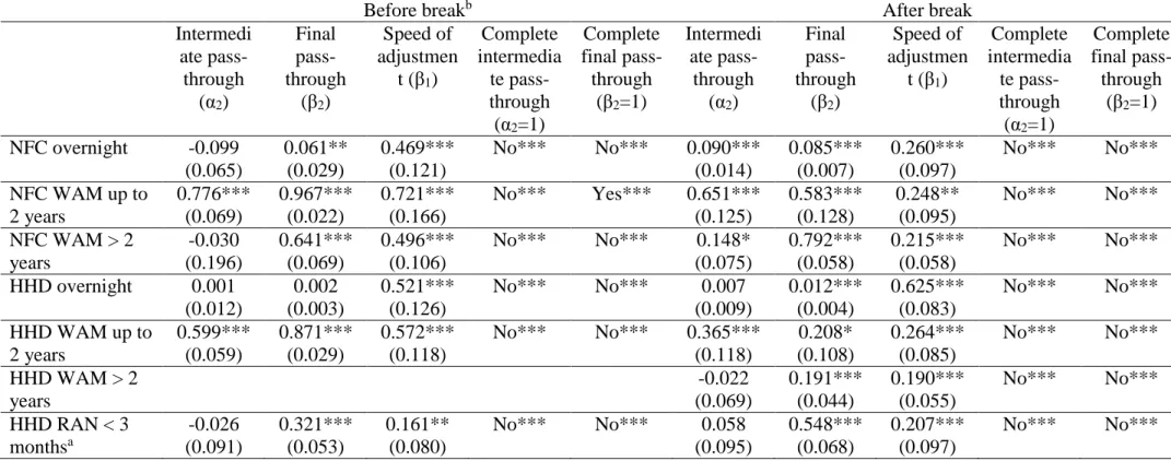
To investigate the change in bank behavior before and after the breaks founded, we split the sample period into two sub-periods using the break date endogenously detected by the test of Andrews (1993). We, therefore, only assume one break in the IRPT since our sample only counts 140 observations which is too small for a division into three subsamples. Note that for
16
the same reason, we choose November 2008 as the break date for interest rate on deposits to enterprises with agreed maturity less than two years. Results of estimation of equation (3) before and after the breaks detected are summarized in Table 6.
As we can remark, the long run pass-through are lower for deposits to firms with agreed maturity more than two years and to households up to two years. Furthermore, we can see that the speed of adjustment is lower after the break in most of regressions, suggesting that banks take more time to adjust their interest rates to driving market reference rates.
We propose two interpretations of these results. The first one is linked with the "near" zero rate interest policy conduct by the European Central Bank (ECB) since the end of 2009. It seems that banks behavior change at that time and that banks decide not to pass all the decrease in interest rate on deposit rates. The second interpretation is linked with the new regulatory requirement on liquidity that will be imposed by Basel III. According to these liquidity requirements, it appears that deposits are now a vital stable resource of liquidity for banks that may be ready to pay for it.
17
Table 6: Retail interest rate on deposits pass-through process based on a univariate error-correction model before and after the detected break
Before breakb After break
Intermedi ate pass-through (α2) Final pass-through (β2) Speed of adjustmen t (β1) Complete intermedia te pass-through (α2=1) Complete final pass-through (β2=1) Intermedi ate pass-through (α2) Final pass-through (β2) Speed of adjustmen t (β1) Complete intermedia te pass-through (α2=1) Complete final pass-through (β2=1) NFC overnight -0.099 (0.065) 0.061** (0.029) 0.469*** (0.121) No*** No*** 0.090*** (0.014) 0.085*** (0.007) 0.260*** (0.097) No*** No*** NFC WAM up to 2 years 0.776*** (0.069) 0.967*** (0.022) 0.721*** (0.166) No*** Yes*** 0.651*** (0.125) 0.583*** (0.128) 0.248** (0.095) No*** No*** NFC WAM > 2 years -0.030 (0.196) 0.641*** (0.069) 0.496*** (0.106) No*** No*** 0.148* (0.075) 0.792*** (0.058) 0.215*** (0.058) No*** No*** HHD overnight 0.001 (0.012) 0.002 (0.003) 0.521*** (0.126) No*** No*** 0.007 (0.009) 0.012*** (0.004) 0.625*** (0.083) No*** No*** HHD WAM up to 2 years 0.599*** (0.059) 0.871*** (0.029) 0.572*** (0.118) No*** No*** 0.365*** (0.118) 0.208* (0.108) 0.264*** (0.085) No*** No*** HHD WAM > 2 years -0.022 (0.069) 0.191*** (0.044) 0.190*** (0.055) No*** No*** HHD RAN < 3 monthsa -0.026 (0.091) 0.321*** (0.053) 0.161** (0.080) No*** No*** 0.058 (0.095) 0.548*** (0.068) 0.207*** (0.097) No*** No***
Note: NFC: Non-Financial Corporations; HHD: Households; WAM: with agreed maturity; RAN: redeemable at notice. *, **, *** denote significance at the 10 %, 5 % and 1 % levels, respectively.
The figures in parentheses are Newey–West HAC standard errors.
18
5. Conclusion
The main contributions of our paper consists of applying the new method for calculating bank output proposed by Wang and Basu (2011) and Colangelo and Inklaar (2012) for a specific country, during a period that includes financial distress, to test its robustness and relevance compared to the method currently used by the SNA and trying to find explanations for negative values found using the new method on FISIM on deposits since 2009.
In line with previous studies on the U.S. and on the Eurozone, we find that the traditional SNA method leads to an overestimation of the value of FISIM for France, especially in a time of financial crisis. The magnitude of this overestimation depends on the values of the term and the risk premium. We show that the proposed new method is robust to the reference rate chosen to compute the term premium, and to periods of market stress. Finally, we obtain negative FISIM on deposit from 2009. Using structural break methodology, we show that these negative FISIM may be explained by a change in interest rate pass-through after the crisis. Especially, it seems that banks offered (and still do) deposit rates higher than money market rates to improve their liquidity positions.
19
Appendix
Table A-1: Results of ADF and KPSS stationarity tests for reference market rates
ADF test KPSS test
Level Trend Level Trend
Constant Trend Constant Trend Constant Trend Constant Trend Eonia -1.61 -2.70 -4.86*** -4.83*** 1.15*** 0.11 0.08 0.06 Euribor 1 month -1.14 -2.17 -7.28*** -7.26*** 1.07*** 0.13* 0.08 0.06 Euribor 2 months -1.53 -2.52 -5.68*** -5.66*** 1.03*** 0.13* 0.08 0.06 Euribor 3 months -1.57 -2.51 -5.53*** -5.51*** 0.99*** 0.14* 0.08 0.06 Euribor 4 months -1.78 -2.92 -4.94*** -5.03*** 0.78*** 0.14* 0.10 0.05 Euribor 5 months -1.61 -2.62 -5.00*** -5.10*** 0.77*** 0.14* 0.10 0.06 Euribor 6 months -1.71 -2.60 -5.34*** -5.32*** 0.94*** 0.15** 0.08 0.06 Euribor 7 months -1.62 -2.62 -5.63*** -5.66*** 0.74** 0.14** 0.10 0.05 Euribor 8 months -1.61 -2.61 -5.72*** -5.76*** 0.73** 0.14** 0.10 0.05 Euribor 9 months -1.75 -2.59 -5.49*** -5.47*** 0.92*** 0.15** 0.07 0.06 Euribor 10 months -1.62 -2.60 -5.89*** -5.92*** 0.71** 0.14* 0.10 0.05 Euribor 11 months -1.63 -2.60 -5.96*** -6.00*** 0.71** 0.13* 0.10 0.05 Euribor 12 months -1.77 -2.59 -5.68*** -5.67*** 0.91*** 0.15** 0.07 0.06 GB 1 year -1.43 -2.16 -7.35*** -7.30*** 1.18*** 0.13* 0.07 0.06 GB 2 years -1.19 -2.22 -9.36*** -9.34*** 1.26*** 0.15** 0.06 0.05 GB 3 years -1.22 -2.38 -9.70*** -9.67*** 1.33*** 0.17** 0.06 0.05 GB 4 years -1.11 -2.47 -9.87*** -9.84*** 1.37*** 0.19** 0.07 0.05 GB 5 years -1.07 -2.61 -9.85*** -9.82*** 1.38*** 0.19** 0.09 0.06 GB 6 years -1.04 -2.59 -9.64*** -9.62*** 1.35*** 0.22*** 0.07 0.06 GB 7 years -0.90 -2.64 -10.30*** -10.28*** 1.44*** 0.20** 0.08 0.05 GB 8 years -0.82 -2.59 -9.91*** -9.90*** 1.37*** 0.21** 0.09 0.06 GB 9 years -0.76 -2.75 -9.26*** -9.26*** 1.38*** 0.20** 0.10 0.06 GB 10 years -0.26 -2.57 -9.62*** -9.63*** 1.45*** 0.18** 0.12 0.08 GB 15 years -0.51 -2.35 -10.83*** -10.83*** 1.42*** 0.17** 0.12 0.06 GB 20 years -0.47 -1.91 -11.51*** -11.50*** 1.42*** 0.16** 0.10 0.08 GB 30 years -0.738 -2.317 -11.800*** -11.779*** 1.480*** 0.135* 0.079 0.082
Note: *, **, *** denotes significance at 10 % level, 5 % level and 1 % level, respectively. The lag parameters for ADF tests are selected based on the Schwartz information criteria. Critical values for the null hypothesis of stationarity (KPSS test) are taken from Kwiatkowski et al. (1992, table 1).
20
Table A-2: Results of ADF and KPSS stationarity tests for bank loan rates
ADF test KPSS test
Level First difference Level First difference Constant Trend Constant Trend Constant Trend Constant Trend NFC < 1 year -1.49 -2.45 -5.77*** -5.79*** 0.54** 0.19** 0.09 0.07 NFC 1-5 years -0.95 -2.05 -14.40*** -14.46*** 0.82*** 0.19** 0.15 0.05 NFC > 5 years -1.40 -2.11 -3.85*** -3.86*** 0.66** 0.14* 0.09 0.08 HHD_HP < 1 year -1.25 -1.64 -4.87*** -4.87*** 0.50** 0.21** 0.11 0.08 HHD_HP 1-5 years -1.85 -2.08 -3.91*** -3.90** 0.41* 0.17** 0.11 0.11 HHD_HP 5-10 years -1.72 -1.85 -3.04** -3.01** 0.73** 0.20** 0.11 0.12* HHD_HP > 10 years -1.83 -2.26 -3.48*** -3.47** 0.63** 0.17** 0.11 0.10 HHD_CC < 1 year -1.64 -1.632 -15.09*** -15.05*** 0.16 0.16** 0.11 0.11* HHD_CC 1-5 years -1.05 -2.15 -14.39*** -14.36*** 1.17*** 0.17** 0.07 0.07 HHD_CC > 5 years -0.28 -2.25 -7.03*** -7.05*** 1.01*** 0.12* 0.11 0.08 HHD_OP < 1 year -0.88 -1.99 -14.80*** -14.74*** 1.11*** 0.15** 0.08 0.06 HHD_OP 1-5 years -0.53 -1.91 -11.65*** -11.62*** 1.20*** 0.10 0.08 0.06 HHD_OP > 5 years -0.90 -1.38 -14.43*** -14.38*** 0.64** 0.22*** 0.19 0.16**
Note: NFC: Non-Financial Corporations; HHD: Households; HP: for house purchase; CC: for consumer credits; OP: for other purposes. *, **, *** denotes significance at 10 % level, 5 % level and 1 % level, respectively. The lag parameters for ADF tests are selected based on the Schwartz information criteria. Critical values for the null hypothesis of stationarity (KPSS test) are taken from Kwiatkowski et al. (1992, table 1).
Table A-3: Results of ADF and KPSS stationarity tests for bank deposits rates
ADF test KPSS test
Level First difference Level First difference Constant Trend Constant Trend Constant Trend Constant Trend NFC Overnight -1.445 -1.616 -13.658*** -13.629*** 0.325 0.180** 0.142 0.114 NFC WAM < 2 years -1.843 -2.415 -3.921*** -3.926** 0.614** 0.183** 0.091 0.070 NFC WAM > 2 years -1.469 -1.828 -14.604*** -14.534*** 0.463** 0.243*** 0.119 0.063 HHD Overnight -2.077 -3.338* -13.211*** -13.198*** 0.904*** 0.211** 0.207 0.137* HHD WAM < 2 years -2.146 -2.274 -4.521*** -4.509*** 0.297 0.173** 0.080 0.072 HHD WAM > 2 years -3.105** -3.118 -13.867*** -13.854*** 0.359* 0.086 0.107 0.079 HHD RAN < 3 months -1.904 -3.031 -5.177*** -5.242*** 0.714** 0.113 0.121 0.042
Note: NFC: Non-Financial Corporations; HHD: Households; WAM: with agreed maturity; RAN: redeemable at notice. *, **, *** denotes significance at 10 % level, 5 % level and 1 % level, respectively. The lag parameters for ADF tests are selected based on the Schwartz information criteria. Critical values for the null hypothesis of stationarity (KPSS test) are taken from Kwiatkowski et al. (1992, table 1).
21
Table A-4: Value of the Schwartz information criterion (BIC) from the error correction estimations (model selection)
LOANS
Non-financial corporations Households for house purchases Households for consumer credit Households other purposes <1 year 1-5 years >5 years <1 year 1-5 years 5-10 years >10 years <1 year 1-5 years >5 years <1 year 1-5 years >5 years
Eonia -119,1 -276,6 -11,73 -8,471 euribor1m -163,9 -284,7 -15,01 -4,108 euribor2m -167,1 -288,4 -16,04 -2,039 euribor3m -175,7 -293,3 -17,59 -0,029 euribor4m -56,75 -236,1 -10,34 20,89 euribor5m -56,75 -236,3 -10,54 20,81 euribor6m -170,8 -303 -17,99 1,285 euribor7m -56,78 -236,8 -10,97 20,92 euribor8m -56,76 -237 -10,88 20,97 euribor9m -164,7 -308,4 -17,98 1,69 euribor10m -56,72 -237,4 -11,03 21,1 euribor11m -56,73 -237,6 -11,13 21,15 euribor12m -157,5 -312,7 -17,7 2,342 gb1y -40,02 -307,8 -161,3 -124,7 gb2y -41,36 -307,6 -166,5 -126,4 gb3y -39,66 -301,3 -166,9 -127,6 gb4y -38,65 -299,1 -168 -128,1 gb5y -37,36 -211,5 -298,5 -294,1 -168,2 -228,2 -128,8 -185 gb6y -206,3 -287,9 -213,2 -185,4 gb7y -204,6 -284,7 -229,8 -185,8 gb8y -202 -279,9 -213,8 -185,5 gb9y -200,3 -276,4 -214,6 -185,3 gb10y -199,7 -274,4 -358,6 -230,4 -185,5 gb15y -195,8 -353,9 -226,6 -186,1 gb20y -190 -343,4 -229,1 -183,6 gb30y -189,4 -336,3 -226 -179,5
22
DEPOSITS Non-financial corporations Households Overnights WAM <2 years WAM >2 years Overnight WAM <2years
WAM> 2 years RAN <3 months Eonia -579,6 -155,9 -682,5 -124,8 -208,8 euribor1m -207 -155,8 -212,9 euribor2m -195,3 -147,8 -213,1 euribor3m -205 -154,2 -213,7 euribor4m -70,41 -79,82 euribor5m -70,33 -79,84 euribor6m -197,8 -150,7 euribor7m -70,19 -79,94 euribor8m -70,1 -79,97 euribor9m -188 -145,3 euribor10m -69,98 -80,03 euribor11m -69,93 -80,07 euribor12m -179,2 -140,7 gb1y -121,4 -99,47 gb2y -102,3 -17,14 -92,53 -152,1 gb3y -15,96 -152 gb4y -15,84 -152,1 gb5y -15,25 -151,4 gb6y -13,42 -151,2 gb7y -12,09 -151 gb8y -10,82 -150,5 gb9y -9,434 -150,3 gb10y -8,65 -150 gb15y -6,173 -149,6 gb20y -3,638 -149,2 gb30y -2,35 -147,8
23
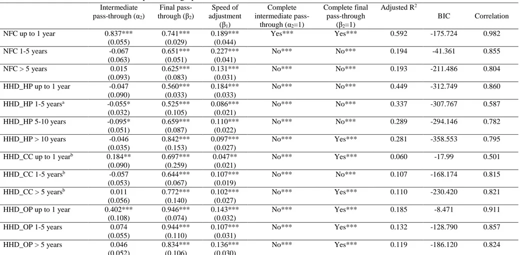
Table A-5: Retail interest rate on loans pass-through process based on a univariate error-correction model
Intermediate pass-through (α2) Final pass-through (β2) Speed of adjustment (β1) Complete intermediate pass-through (α2=1) Complete final pass-through (β2=1) Adjusted R2 BIC Correlation NFC up to 1 year 0.837*** (0.055) 0.741*** (0.029) 0.189*** (0.044) Yes*** Yes*** 0.592 -175.724 0.982 NFC 1-5 years -0.067 (0.063) 0.651*** (0.051) 0.227*** (0.041) No*** No*** 0.194 -41.361 0.855 NFC > 5 years 0.015 (0.093) 0.625*** (0.083) 0.131*** (0.031) No*** No*** 0.193 -211.486 0.804 HHD_HP up to 1 year -0.047 (0.090) 0.560*** (0.033) 0.184*** (0.033) No*** No*** 0.449 -312.749 0.860 HHD_HP 1-5 yearsa -0.055* (0.032) 0.525*** (0.105) 0.086*** (0.021) No*** No*** 0.337 -307.767 0.587 HHD_HP 5-10 years -0.095* (0.051) 0.659*** (0.087) 0.110*** (0.022) No*** No*** 0.289 -294.146 0.782 HHD_HP > 10 years -0.046 (0.035) 0.842*** (0.153) 0.097*** (0.027) No*** Yes*** 0.281 -358.553 0.795 HHD_CC up to 1 yearb 0.184** (0.090) 0.697*** (0.259) 0.047** (0.021) No*** Yes*** 0.060 -17.99 0.501 HHD_CC 1-5 yearsb -0.057 (0.053) 0.644*** (0.067) 0.107*** (0.019) No*** No*** 0.107 -168.174 0.815 HHD_CC > 5 yearsb 0.011 (0.056) 0.772*** (0.140) 0.102*** (0.027) No*** Yes*** 0.110 -230.420 0.821 HHD_OP up to 1 year 0.402*** (0.108) 0.946*** (0.074) 0.143*** (0.032) No*** Yes*** 0.185 -8.471 0.911 HHD_OP 1-5 years 0.074 (0.055) 0.944*** (0.110) 0.107*** (0.031) No*** Yes*** 0.132 -128.790 0.857 HHD_OP > 5 years 0.046 (0.052) 0.834*** (0.106) 0.136*** (0.030) No*** Yes*** 0.119 -186.120 0.824
Note: NFC: Non-Financial Corporations; HHD: Households; HP: for house purchase; CC: for consumer credits; OP: for other purposes. *, **, *** denote significance at the 10 %, 5 % and 1 % levels, respectively. The figures in parentheses are Newey–West HAC standard errors. The sample period is January 2003 to September 2014 unless otherwise specified. Model selection is performed on the basis of the Schwartz criterion (BIC).
24
Table A-6: Retail interest rate on deposits pass-through process based on a univariate error-correction model
Intermediate pass-through (α2) Final pass-through (β2) Speed of adjustment (β1) Complete intermediate pass-through (α2=1) Complete final pass-through (β2=1) Adjusted R2 BIC Correlation NFC overnight 0.079*** (0.014) 0.079*** (0.012) 0.116** (0.049) No*** No*** 0.170 -579.65 0.864 NFC WAM up to 2 years 0.784*** (0.073) 0.785*** (0.036) 0.169*** (0.054) No*** No*** 0.643 -207.007 0.985 NFC WAM > 2 years 0.055 (0.093) 0.601*** (0.086) 0.162*** (0.041) No*** No*** 0.136 -17.14 0.773 HHD overnight -0.003 (0.010) 0.015*** (0.003) 0.391*** (0.092) No*** No*** 0.182 -682.455 0.630 HHD WAM up to 2 years 0.608*** (0.067) 0.520*** (0.091) 0.065*** (0.026) No*** No*** 0.432 -155.755 0.894 HHD WAM > 2 years -0.035 (0.063) 0.201*** (0.049) 0.162*** (0.049) No*** No*** 0.104 -152.115 0.484 HHD RAN < 3 monthsa 0.034 (0.066) 0.459*** (0.057) 0.152** (0.060) No*** No*** 0.188 -213.481 0.838
Note: NFC: Non-Financial Corporations; HHD: Households; WAM: with agreed maturity; RAN: redeemable at notice. *, **, *** denote significance at the 10 %, 5 % and 1 % levels, respectively. The figures in parentheses are Newey–West HAC standard errors. The sample period is January 2003 to September 2014 unless otherwise specified. Model selection is performed on the basis of the Schwartz criterion (BIC).
25
Figure A-1: Sensitivity analysis of the computation of FISIM on deposits
Figure A-2: Sensitivity analysis of the computation of FISIM on loans
-1 0 ,0 0 0 0 1 0 ,0 0 0 2 0 ,0 0 0 2003 2004 2005 2006 2007 2008 2009 2010 2011 2012
FISIM on deposits adjusted from term premium
First best reference rate (SIC) Second best reference rates (SIC)
Reference rates from C&I (2012) Outstanding amount rates
0 1 0 ,0 0 0 2 0 ,0 0 0 3 0 ,0 0 0 4 0 ,0 0 0 2003 2004 2005 2006 2007 2008 2009 2010 2011 2012
FISIM on loans adjusted for term premium
First best reference rates (SIC) Reference rates from C&I (2012)
26
References
Ahmad, N. (2013), FISIM, document presented at presented at the 8th Meeting of the Advisory Expert Group on National Accounts, Luxembourg.
Andrews, D.W.K. (1993), Tests for parameter instability and structural change with an unknown change point, Econometrica 61(4), pp. 821-856.
Bai, J. and Perron, P. (1998), Testing and estimating linear models with multiple structural changes, Econometrica 66(1), pp. 47-78.
Bai, J. and Perrron, P. (2003a), Computation and analysis of multiple structural change models, Journal of Applied Econometrics 18(1), pp. 1-22.
Bai, J. and Perrron, P. (2003b), Critical values for multiple structural change tests, Econometrics Journal 6(1), pp. 72-78.
Bajo-Rubio, O. Diaz-Roldan, C. and Esteve, C. (2008), US deficit sustainability revisited: A multiple structural change approach, Applied Economics 40(12), pp. 1609-1613.
Basu, S., Inklaar, R. and Wang, J. C. (2011). The value of risk: measuring the service output of US commercial banks. Economic Inquiry, 49(1), pp. 226-245.
Beckmann, J., Belke, A. and Kühl, M. (2011), The dollar-euro exchange rate and macroeconomic fundamentals: a time-varying coefficient approach, Review of World Economics 147(1), pp. 11-40.
Chow, G. (1960), Tests of equality Between sets of coefficients in two linear
regressions, Econometrica 28(3), pp. 591–605.
Colangelo, A (2012), Measuring FISIM in the euro area under various choices of reference rate, Joint National Accounts Meeting, ECB.
Colangelo, A. and Inklaar, R. (2012), Bank output measurement in the Euro area: A modified approach, Review of Income and Wealth 58(1), pp. 142-165.
Cullen, D. (2011), A Progress Report on ABS Investigations Into FISIM in the National Accounts, the Consumer Price Index and Balance of Payments. Document presented at the Meeting of the Task Force on Financial Intermediation Services Indirectly Measured (FISIM), IMF, Washington D.C.
Davies, M. (2010), The measurement of financial services in the national accounts and the financial crisis, IFC Bulletin chapters, 33, pp. 350-357.
De Bondt, G.J. (2002), Retail bank interest rate pass-through: New evidence at the Euro area level, ECB Working paper 136, European central bank, Frankfurt.
De Bondt, G.J. (2005), Interest rate pass-through: Empirical results for the Euro area, German Economic Review 6(1), pp. 37-78.
27
De Bondt, G.J., Mojon, B. and Valla, N. (2005), Term structure and the sluggishness of retail bank rates in Euro area countries, ECB Working paper 518, European central bank, Frankfurt. Diewert, W. E., Fixler, D. and Zieschang, K. (2012), Problems with the Measurement of Banking Services in a National Accounting Framework. UNSW Australian School of Business Research Paper No. 2012-25.
Diewert, W. E. (2013). Voyage Accounting, User Costs and the Treatment of Financial Transactions in the Theory of the Firm, Discussion Paper 13-03.
Engle, R.F. and Granger, C.W.J. (1987), Cointegration and error correction: representation, estimation, and testing, Econometrica 55(2), pp. 251-276.
European Central Bank (2003), Manual on MFI Interest Rate Statistics. Frankfurt
Fixler, D.J., Reinsdorf, M.B. and Villones S. (2010), Measuring the services of commercial banks in the NIPA, Bank for International Settlements, IFC Bulletin, n°33, July, 346-348. Fournier J.M. and Marionnet D. (2010), L'activité bancaire mesurée par les banques et la comptabilité nationale : des différences riches d'enseignements, Insee première, 1285.
Hansen, B.E. (1992), Tests for parameter instability in regressions with I(1) processes, Journal of Business & Economic Statistics 10(3), pp. 321-335.
Hansen, B.E. (1997), Approximate asymptotic p values for structural-change tests, Journal of Business & Economic Statistics 15(1), pp. 60-67.
Hofmann, B. and Mizen, P. (2004), Interest rate pass-through and monetary transmission: Evidence from individual financial institution’s retail rates, Economica 71(281), pp. 99-124. Inklaar, R. and Wang, J. C. (2013), Real Output of Bank Services: What Counts is What Banks Do, Not What They Own. Economica, 80, pp. 96–117.
Intersecretariat Working Group on National Accounts (ISWGNA) (2013), ISWGNA Task Force on FISIM, final report presented at the 8th Meeting of the Advisory Expert Group on National Accounts, Luxembourg.
Kejriwal, M. and Perron, P. (2010), Testing for multiple structural changes in cointegrated regression models, Journal of Business & Economic Statistics 28(4), pp. 503-522.
Kwiatkowski, D., Phillips, P.C.B., Schmidt, P. and Shin, Y. (1992), Testing the null hypothesis of stationarity against the alternative of a unit root: How sure are we that economic time series have a unit root?, Journal of Econometrics 54(1-3), pp. 159-178.
Maddala, G.S. and Kim, I.M. (1998), Unit roots, cointegration, and structural change. Cambridge University Press: Cambridge, UK.
Marotta, G. (2009), Structural breaks in the lending interest rate pass-through and the euro, Economic Modelling 26(1), pp. 191-205.
28
Mink, R (2008), An Enhanced Methodology of Compiling Financial Intermediation Services Indirectly Measured (FISIM), paper presented at OECD Working Party on National Accounts, Paris.
Mink, R. (2010), Mesure et enregistrement des services financiers, document presented at Colloque de l’Association de comptabilité nationale, Paris.
Organization for Economic Cooperation and Development (1998), FISIM. In Joint OECD/ESCAP Meeting on National Accounts.
Philippon, T., & Reshef, A., 2013. An international look at the growth of modern finance. The Journal of Economic Perspectives, pp. 73-96.
Ruggles, R. (1983), The United States National Income Accounts, 1947-77: Their Conceptual Basis and Evolution, in The U.S. National Income and Product Accounts: Selected Topics, Murray F. Foss, ed., University of Chicago Press, Chicago and London, pp. 15-104.
Sakuma, I. (2013), A note on FISIM, forthcoming in Price and Productivity Measurement: Volume 3—Services, W. Erwin Diewert, Bert M. Balk, Dennis Fixler, Kevin J. Fox and Alice O. Nakamura (eds.), Trafford Press .
Sander, H. and Kleimeier, S. (2004), Convergence in euro-zone retail banking? What interest rate pass-through tells us about monetary policy transmission, competition and integration, Journal of International Money and Finance 23(3), pp. 461-492.
Schreyer, P. (2009), Comment on "A General-Equilibrium Asset-Pricing Approach to the Measurement of Nominal and Real Bank Output", Chapter in Price Index Concepts and Measurement, ed. by E. Diewert, J. Greenlees, and C. Hulten. Chicago: University of Chicago Press for NBER, pp. 320-328.
Schreyer, P. and Stauffer, P. (2011), Measuring the Production of Financial Corporations, forthcoming in Price and Productivity Measurement: Volume 3; Services, W.E. Diewert, B.M. Balk, D. Fixler, K.J. Fox and A.O. Nakamura (eds.).
Sørensen, C. K. and Werner, T. (2006). Bank interest rate pass-through in the euro area: a cross country comparison. ECB Working paper 580, European central bank, Frankfurt.
United Nations, Eurostat, International Monetary Fund, Organization for Economic Cooperation and Development and World Bank (1993), System of National Accounts 1993, United Nations, New York.
United Nations, Eurostat, International Monetary Fund, Organization for Economic Cooperation and Development and World Bank (2008), System of National Accounts 2008, United Nations, New York.
Vanoli A. (2005), A History of National Accounting. IOS Press: Amsterdam.
Wang, J. C. (2003), Loanable Funds, Risk, and Bank Service Output, Federal Reserve Bank of Boston, Working Paper Series, No. 03-4.