Modeling the variability of electrical activity in the brain

HAL Id: tel-01175851

https://tel.archives-ouvertes.fr/tel-01175851

HAL is a multi-disciplinary open access archive for the deposit and dissemination of sci-entific research documents, whether they are pub-lished or not. The documents may come from teaching and research institutions in France or

L’archive ouverte pluridisciplinaire HAL, est destinée au dépôt et à la diffusion de documents scientifiques de niveau recherche, publiés ou non, émanant des établissements d’enseignement et de recherche français ou étrangers, des laboratoires

Sebastian Hitziger

To cite this version:

Sebastian Hitziger. Modeling the variability of electrical activity in the brain. Other. Université Nice Sophia Antipolis, 2015. English. �NNT : 2015NICE4015�. �tel-01175851�

PhD THESIS

prepared at

Inria Sophia Antipolis

and presented at the

University of Nice-Sophia Antipolis

Graduate School of Information and Communication

Sciences

A dissertation submitted in partial fulfillment

of the requirements for the degree of

DOCTOR OF SCIENCE

Specialized in Control, Signal and Image Processing

Modeling the Variability of

Electrical Activity in the Brain

Sebastian HITZIGER

Advisors Th´eodore Papadopoulo Inria Sophia Antipolis, France Maureen Clerc Inria Sophia Antipolis, France Reviewers Bruno Torr´esani University of Aix-Marseille, France

Alain Rakotomamonjy University of Rouen, France Examiners Laure Blanc-F´eraud Inria Sophia Antipolis, France

Christian G. B´enar University of Aix-Marseille, France Invited Jean-Louis Divoux Axonic, Vallauris, France

UNIVERSIT´

E DE NICE-SOPHIA ANTIPOLIS

´

ECOLE DOCTORALE STIC

Sciences et Technologies de l’Information et de la Communication

TH`

ESE

pour l’obtention du grade de

DOCTEUR EN SCIENCES

de l’Universit´e de Nice-Sophia Antipolis

Discipline: Automatique, Traitement du Signal et des Images

pr´esent´ee et soutenue par

Sebastian HITZIGER

Mod´

elisation de la variabilit´

e de

l’activit´

e ´

electrique dans le cerveau

Date de soutenance : 14 avril 2014

Composition du jury:

Directeurs Th´eodore Papadopoulo Inria Sophia Antipolis, France Maureen Clerc Inria Sophia Antipolis, France Rapporteurs Bruno Torr´esani Universit´e d’Aix-Marseille, France

Alain Rakotomamonjy Universit´e de Rouen, France Examinateurs Laure Blanc-F´eraud Inria Sophia Antipolis, France

Christian G. B´enar Universit´e d’Aix-Marseille, France Invit´e Jean-Louis Divoux Axonic, Vallauris, France

Abstract

This thesis investigates the analysis of brain electrical activity. An impor-tant challenge is the presence of large variability in neuroelectrical record-ings, both across different subjects and within a single subject, for example across experimental trials. We propose a new method called adaptive wave-form learning (AWL). It is general enough to include all types of relevant variability empirically found in neuroelectric recordings, but it can be spe-cialized for different concrete settings to prevent from overfitting irrelevant structures in the data.

The first part of this work gives an introduction into the electrophysiol-ogy of the brain, presents frequently used recording modalities, and describes state-of-the-art methods for neuroelectrical signal processing.

The main contribution of the thesis consists in three chapters introduc-ing and evaluatintroduc-ing the AWL method. We first provide a general signal decomposition model that explicitly includes different forms of variability across signal components. This model is then specialized for two concrete applications: processing a set of segmented experimental trials and learn-ing repeatlearn-ing structures across a slearn-ingle recorded signal. Two algorithms are developed to solve these models. Their efficient implementations, based on alternate minimization and sparse coding techniques, allow the processing of large datasets.

The proposed algorithms are evaluated on both synthetic data and real data containing epileptiform spikes. Their performances are compared to those of PCA, ICA, and template matching for spike detection.

Keywords: electroencephalography (EEG), event-related poten-tials (ERP), epileptiform spikes, signal variability, dictionary learn-ing, sparse coding

R´esum´e

Cette th`ese explore l’analyse de l’activit´e ´electrique du cerveau. Un d´efi im-portant de ces signaux est leur grande variabilit´e `a travers diff´erents essais et/ou diff´erents sujets. Nous proposons une nouvelle m´ethode appel´ee adap-tive waveform learning (AWL). Cette m´ethode est suffisamment g´en´erale pour permettre la prise en compte de la variabilit´e empiriquement rencon-tr´ee dans les signaux neuro´electriques, mais peut ˆetre sp´ecialis´ee afin de pr´evenir l’overfitting du bruit.

La premi`ere partie de ce travail donne une introduction sur l’´electrophy-siologie du cerveau, pr´esente les modalit´es d’enregistrement fr´equemment utilis´ees et d´ecrit l’´etat de l’art du traitement de signal neuro´electrique.

La principale contribution de cette th`ese consiste en 3 chapitres intro-duisant et ´evaluant la m´ethode AWL. Nous proposons d’abord un mod`ele de d´ecomposition de signal g´en´eral qui inclut explicitement diff´erentes formes de variabilit´e entre les composantes de signal. Ce mod`ele est ensuite sp´e-cialis´e pour deux applications concr`etes: le traitement d’une s´erie d’essais exp´erimentaux segment´es et l’apprentissage de structures r´ep´et´ees dans un seul signal. Deux algorithmes sont d´evelopp´es pour r´esoudre ces probl`emes de d´ecomposition. Leur impl´ementation efficace bas´ee sur des techniques de minimisation altern´ee et de codage parcimonieux permet le traitement de grands jeux de donn´ees.

Les algorithmes propos´es sont ´evalu´es sur des donn´ees synth´etiques et r´eelles contenant des pointes ´epileptiformes. Leurs performances sont com-par´ees `a celles de l’ACP, l’ICA, et du template-matching pour la d´etection des pointes.

Mots cl´es : ´electroencephalographie (EEG), potentiels ´evoqu´es (ERP), pointes ´epileptiformes, variabilit´e du signal, apprentissage de dictionnaires, codage parcimonieux

Acknowledgements

First of all, I would like to express my deep gratitude towards my supervisors Th´eo Papadopoulo and Maureen Clerc for accompanying me throughout the past three years with their expertise, thoughtful advice, and encouraging support. I would also like to thank Rachid Deriche and the Athena team at Inria for welcoming me and giving me such an inspiring environment.

I am very grateful to Alain Rakotomamonjy and Bruno Torr´esani for taking a significant amount of their time to review this thesis and share with me their insightful suggestions and remarks. Furthermore, I would like to thank Laure Blanc-F´eraud and Christian B´enar for their participation in the jury.

Much of the present work grew out of ideas coming from the fruitful exchange with the members of the two ANR1 _{projects Coadapt and}

Multi-model. In particular, I would like to thank: Christian B´enar for his great enthusiasm which encouraged me to pursue the detailed investigation of neurovascular coupling; Sandrine Saillet and the experimentalists for the great and rich datasets which allowed us to obtain many interesting find-ings; Bruno Torr´esani for inspiring discussions on various signal processing topics; Alexandre Gramfort for his helpful suggestions on dictionary learn-ing.

I am extremely grateful to all my friends and colleagues in the Athena and Neuromathcomp team who made this PhD a wonderful time: Emmanuel O., Emmanuel C., Sylvain, Anne-Charlotte, Joan, Auro, Dieter, Eoin, Has-san, Romain, James R., James I., Antoine, Gabriel and Sara, Elodie, Gon-zalo, Kartheek, Li, Nathan¨el, Rutger, Marco, Demian, Lola. Very special thanks go to Christos for discussing multi-channel dictionary learning and sharing his results; to Jaime, Brahim, and Asya for putting up with me as an office mate; to Claire for kindly helping me through all those administrative issues; to James M. for those deep philosophical discussions and being the best flatmate one could imagine; and to my dear friend Rodrigo for sharing with me the pleasant bike rides to the office.

Finally, I would like to thank my family for all their love and support throughout this thesis.

1

Contents

Introduction en fran¸cais 1

Contributions . . . 3 Sommaire . . . 4 Notations . . . 8 1 Introduction 9 1.1 Contributions . . . 10 1.2 Outline . . . 12 1.3 Notation . . . 14

2 Analyzing Brain Electrical Activity 15 2.1 Introduction . . . 16

2.2 Electrophysiology of the brain . . . 16

2.3 Recording electromagnetic activity . . . 18

2.3.1 Electroencephalography (EEG) . . . 18

2.3.2 Intracranial recordings . . . 19

2.3.3 Magnetoencephalography (MEG) . . . 21

2.3.4 Complementary measurements of EEG and MEG . . . 21

2.4 Recording metabolism and hemodynamics . . . 22

2.5 Neuroelectrical signals . . . 23

2.5.1 Event-related potentials (ERPs) . . . 24

2.5.2 Spontaneously repeating activity (SRA) . . . 25

2.6 Signal analysis: goals and challenges . . . 27

2.6.1 Assessing variability . . . 27

2.6.2 Compact and interpretable representation . . . 28

2.6.3 Flexible algorithm . . . 29

2.7 Example dataset: multi-modal recordings . . . 29

3 Neuroelectrical Signal Processing 33 3.1 Introduction and overview . . . 34

3.3 Models with temporal variability . . . 37

3.3.1 Woody’s method . . . 37

3.3.2 Dynamic time warping . . . 38

3.3.3 Variable response times . . . 40

3.4 Linear multi-component models . . . 40

3.4.1 Principal component analysis (PCA) . . . 41

3.4.2 Independent component analysis (ICA) . . . 42

3.5 Combined approaches . . . 45

3.5.1 Differentially variable component analysis (dVCA) . . 45

3.6 Sparse representations . . . 46

3.6.1 Sparse coding and time-frequency representations . . . 46

3.6.2 Dictionary learning . . . 50

3.6.3 Translation-invariant dictionary learning . . . 50

3.7 Conclusion and outlook . . . 52

4 Adaptive Waveform Learning (AWL) 53 4.1 Introduction . . . 54

4.2 Modeling variability . . . 54

4.2.1 Linear operations on signal components . . . 55

4.2.1.1 Translations . . . 56 4.2.1.2 Dilations . . . 57 4.3 AWL model . . . 57 4.3.1 General model . . . 57 4.3.2 Sparse coefficients . . . 58 4.3.3 Minimization problem . . . 59 4.3.4 Explicit representation . . . 59 4.4 Algorithm AWL . . . 60 4.4.1 Initialization . . . 60 4.4.2 Coefficient updates . . . 61 4.4.3 Waveform updates . . . 62 4.4.4 Waveform centering . . . 63

4.5 Relation to previous methods . . . 64

4.6 Hyperparameters and hierarchical AWL . . . 65

5 Epoched AWL 67 5.1 Introduction . . . 68 5.2 Model specifications . . . 68 5.2.1 Explicit representation . . . 69 5.3 Algorithm E-AWL . . . 70 5.3.1 Coefficient updates . . . 70 5.3.2 Waveform updates . . . 71 5.3.3 Waveform centering . . . 71

5.3.4 Discrete shifts and boundary issues . . . 72

CONTENTS

5.4.1 Influence of varying amplitudes . . . 76

5.4.2 Influence of varying latencies . . . 76

5.4.3 Robustness to noise . . . 78

5.4.4 Qualitative comparison . . . 78

5.5 Evaluation on LFP recording . . . 79

5.5.1 Preprocessing and epoching . . . 80

5.5.2 Hierarchical representations with epoched AWL . . . . 80

5.5.3 Comparison of PCA, ICA, and AWL . . . 82

6 Contiguous AWL 85 6.1 Introduction . . . 86 6.2 Model specifications . . . 86 6.3 Algorithm C-AWL . . . 88 6.3.1 Coefficient updates . . . 88 6.3.2 Waveform updates . . . 89 6.3.3 Waveform centering . . . 90

6.4 C-AWL for spike learning . . . 91

6.4.1 Multi-class spike learning (MC-Spike) . . . 92

6.4.1.1 Handling overlapping spikes . . . 94

6.4.1.2 Initializing new spikes . . . 94

6.4.1.3 Performance measures . . . 95

6.4.1.4 Experiments . . . 97

6.4.2 Adaptive duration spike learning (AD-Spike) . . . 100

6.4.3 Comparing detection performance . . . 102

6.5 Exploring neuro-vascular coupling . . . 105

7 Conclusion 109 7.1 Strengths and weaknesses of AWL . . . 110

7.2 Future work . . . 111

Conclusion en fran¸cais) 115 Points forts et faibles de AWL . . . 116

Travail futur . . . 117

A Implementation of MP and LARS 121

List of Figures

1 Structure du document et d´ependances entre les chapitres. . . 5

1.1 Document structure and dependencies between chapters . . . 12

2.1 Electrochemical communication between two neurons . . . 16

2.2 Pyramidal neuron assemblies generate electromagnetic field . 17 2.3 First recording of a human EEG . . . 18

2.4 EEG recording session and visualization on the scalp . . . 19

2.5 EEG recording during epileptic seizure . . . 20

2.6 Conoluted arrangement of the cerebral cortex . . . 21

2.7 Spatial and temporal resolution of brain imaging techniques . 23 2.8 Generation of a P300 event-related potential . . . 25

2.9 Brain activity during different sleep stages . . . 26

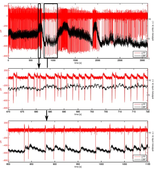
2.10 Simultaneous LFP and CBF recording . . . 30

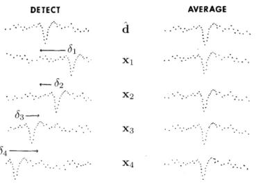
3.1 Averaging over waveforms with latency jitter . . . 36

3.2 Illustration of Woody’s method . . . 38

3.3 Dynamic time warping: illustration of the path . . . 39

3.4 Dynamic time warping applied to auditory evoked responses . 40 3.5 Artifact identification through ICA . . . 44

3.6 Illustration of Gabor atoms . . . 47

3.7 Enhancing induced activity through averaging in time-frequency 49 3.8 Algorithm scheme for dictionary learning . . . 51

5.1 Illustration of waveform shifts on bounded domain . . . 72

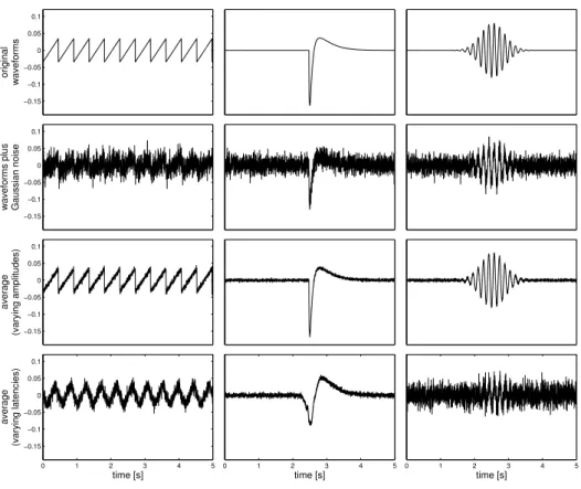
5.2 Simulated waveforms for synthetic experiment . . . 73

5.3 Illustration of simulated noisy trials . . . 74

5.4 Error curves for PCA, ICA, and E-AWL . . . 77

5.5 Waveforms recoverd with PCA, ICA, and E-AWL . . . 79

5.6 Illustration of epoched spikes from original dataset . . . 80

5.7 Hierarchical waveform representation learned with E-AWL . . 81

6.1 Illustration of waveform shifts in a long signal . . . 87

6.2 Two time windows of a typical spike . . . 93

6.3 Subtracting overlapping spikes with matching pursuit . . . . 94

6.4 Spike representations learned with MC-Spike on LFP dataset 96

6.5 Spike representation with MC-Spike (five spike classes) . . . . 98

6.6 Dilatable spike representation learned with AD-Spike . . . 101

6.7 Qualitative comparison between MC-Spike and AD-Spike . . 102

6.8 Detection accuracies: MC-Spike, AD-Spike, template matching104

6.9 Epileptiform spikes synchronizing with CBF activity . . . 106

7.1 Multi-channel extension . . . 112

List of Algorithms

List of Acronyms

AD-Spike Adaptive Duration Spike Learning

ANR L’Agence Nationale de la Recherche

AP Action Potential

AWL Adaptive Waveform Learning

BCI Brain Computer Interface

BOLD Blood Oxygenation Level Dependent

BP Bereitschaftspotential

BSS Blind Source Separation

C-AWL Contiguous AWL

CBF Cerebral Blood Flow

DL Dictionary Learning

DTW Dynamic Time Warping

dVCA Differentially Variable Component Analysis

E-AWL Epoched AWL

ECoG Electrocorticography

EEG Electroencephalography

ERP Event-Related Potential

FFT Fast Fourier Transform

fMRI functional Magnetic Resonance Imaging

GOF Goodness of Fit

ICA Independent Component Analysis

JADE Joint Approximate Diagonalization of Eigenmatrices

LARS Least Angle Regression

Lasso Least Absolute Shrinkage and Selection Operator

LDF Laser Doppler Flowmetry

LFP Local Field Potential

LSR Local Spiking Rate

MC-Spike Multiclass Spike Learning

MEG Magnetoencephalography

MP Matching Pursuit

MUA Multiple-Unit Spike Activity

NIRS Near-Infrared Spectroscopy

OMP Orthogonal Matching Pursuit

PCA Principal Component Analysis

PET Positron Emission Tomography

PSP Postsynaptic Potential

sEEG Stereoelectroencephalography

SNR Signal-to-Noise Ratio

SPECT Single Photon Emission Computed Tomography SQUID Superconducting Quantum Interference Device

SRA Spontaneously Repeating Activity

SSVEP Steady-State Visual-Evoked Potential

SVD Singular Value Decomposition

Introduction en fran¸cais

En 2013, deux projets de recherche d’une dure´e de 10 ans avec plus d’un milliard d’euros de budget chacun, le Human Brain Project et le BRAIN Initivative, ont ´et´e lanc´es respectivement par l’UE et les Etats-Unis. Visant `

a simuler le cerveau humain `a l’aide de supercalculateurs, ces projets t´e-moignent du grand int´erˆet scientifique `a une meilleure compr´ehension des m´ecanismes sous-jacents au cerveau.

Les avanc´ees r´esultant du progr`es dans la recherche en neurosciences ont ´et´e nombreuses. Outre l’am´elioration constante du traitement des trou-bles mentaux ´etudi´es depuis longtemps comme l’´epilepsie, la d´emence, la maladie de Parkinson ou la d´epression, le d´eveloppement technologique a conduit `a de nombreuses nouvelles applications des neurosciences. `A titre d’exemple, les interfaces cerveau-ordinateur (BCI) permettent d’utiliser les ondes c´er´ebrales d’un utilisateur pour communiquer avec un dispositif ex-terne. Le BCI peut ainsi aider les personnes handicap´ees ou non dans l’ex´ecution de diverses tˆaches cognitives ou sensori-motrices.

`

A bien des ´egards, ces progr`es sont dˆus `a la large gamme de modalit´es d’imagerie c´er´ebrale qui sont aujourd’hui disponibles, comprenant (parmi plusieurs autres) l’´electro- et la magn´etoenc´ephalographie (EEG / MEG), l’imagerie par r´esonance magn´etique fonctionnelle (IRMf), la tomographie par ´emission des positons (TEP), la tomographie d’´emission monophotonique (TEMP), et la spectroscopie proche infrarouge (NIRS). Avec la possibilit´e d’acqu´erir `a haute r´esolution des enregistrements multimodaux vient aussi le d´efi de l’interpr´etation de ces donn´ees de mani`ere ad´equate. Cela n´ecessite tout d’abord la conception de mod`eles physiologiques expliquant la g´en´era-tion de ces signaux. Des m´ethodes sophistiqu´ees de traitement du signal sont ensuite n´ecessaires pour, sur la base de ces mod`eles, repr´esenter des signaux avec des informations significatives et statistiquement pertinentes.

Le pr´esent travail se concentre sur l’analyse des enregistrements neu-ro´electriques. L’une des techniques fondamentales de traitement de ces sig-naux se base sur la moyenne d’un grand nombre de sigsig-naux enregistr´es dans des conditions similaires. Cette m´ethode, introduite par George D.

Daw-son (Dawson,1954), s’est montr´ee utile pour d´etecter les potentiels ´evoqu´es (ERP) de petites amplitudes, qui seraient cach´es sous le bruit et l’activit´e de fond des neurones avec un seul enregistrement. Bien que cette technique soit encore souvent utilis´ee pour analyser les ERPs, les hypoth`eses sous-jacentes au calcul de la moyenne ont ´et´e contest´ees et montr´ees inexactes dans de nombreux contextes (Coppola et al., 1978; Horvath, 1969; Truccolo et al.,

2002).

Un probl`eme principal est l’observation que les r´eponses neurales ont tendance `a varier en amplitude, en latence et mˆeme en forme (Jung et al.,

2001; Kisley and Gerstein, 1999). Cette variabilit´e existe entre diff´erents sujets, mais aussi pour un mˆeme sujet entre diff´erents essais exp´erimentaux. Compenser la variabilit´e des signaux du cerveau peut permettre une meilleure caract´erisation de la r´eponse neurale st´er´eotype `a un ph´enom`ene sous-jacent. En outre, la description et la quantification de la variabil-it´e, inter ou intra-sujet, sont des sources pr´ecieuses d’information. Par exemple, la diminution des amplitudes de la r´eponse `a travers une session d’enregistrement peut ˆetre un signe d’effets de fatigue ou d’accoutumance du sujet. Une des premi`eres extensions de l’approche de Dawson est la m´ethode de Woody (Woody,1967) qui prend en compte diff´erentes latences pendant le calcul de la moyenne. Ces derni`eres d´ecennies, un large ´eventail de mod-`eles et de techniques a ´et´e propos´e pour tenir compte des diff´erents aspects de variabilit´e. Les techniques de d´ecomposition lin´eaire comme l’ACP et l’ICA peuvent compenser des changements en amplitude alors que d’autres techniques comme le dynamic time warping consid´erent des d´eformations plus g´en´erales de la forme du signal.

Outre la comptabilisation ad´equate de la variabilit´e, il y a plusieurs autres caract´eristiques qu’un outil id´eal de traitement de signal neuro´elec-trique devrait poss´eder. Les enregistrements, qui sont souvent acquis dans plusieurs dimensions (par exemple, de multiples essais exp´erimentaux, ca-naux ou modalit´es), n´ecessitent l’extraction efficace d’informations perti-nentes dans une repr´esentation compacte qui permet une interpr´etation facile. Il est indespensable d’incorporer dans le mod`ele toutes les informa-tions pr´ealables afin d’´eviter l’extraction de structures de signaux non per-tinentes. D’un autre cˆot´e, les formes exactes des r´eponses neurales sont sou-vent inconnues, ce qui rend n´ecessaire l’apprentissage de ces formes d’onde aussi aveugl´ement (c’est-`a-dire, sans a priori) que possible. En raison de ces diff´erentes exigences compl´ementaires, la conception d’une m´ethode op-timale est une tˆache difficile.

L’objectif de cette th`ese est de fournir un cadre de d´ecomposition des signaux mod´elisant explicitement la variabilit´e rencontr´ee dans les enregis-trements neuro´electriques. Grˆace `a sa formulation g´en´erale, ce cadre peut ˆetre adapt´e `a une vari´et´e de diff´erentes tˆaches de traitement du signal.

INTRODUCTION EN FRAN ¸CAIS

Contributions

Le r´esultat principal de cette th`ese est la conception d’une m´ethode, ap-pel´e adaptive waveform learning (AWL), pour traiter des signaux neuro´elec-triques. La nouveaut´e de cette approche est la mod´elisation explicite de la variabilit´e des composantes des signaux par des transformations math´ema-tiques.

La m´ethode AWL est tout d’abord pr´esent´ee au Chapitre 4 de fa¸on th´eorique. On consid`ere un mod`ele tr`es g´en´eral de d´ecomposition o`u la variabilit´e est repr´esent´ee par des transformations lin´eaires arbitraires. Ce mod`ele sert de cadre g´en´eral pour diff´erentes applications neuro´electriques et peut ˆetre vu comme une g´en´eralisation de diff´erents mod`eles existants. Dans ce cadre, nous ne fournissons pas d’impl´ementation concr`ete. Cependant, nous pr´esentons un algorithme g´en´erique qui peut ˆetre utilis´e comme une re-cette pour impl´ementer de telles applications concr`etes. Comme AWL repose sur un mod`ele parcimonieux, l’algorithme g´en´erique peut ˆetre efficacement impl´ement´e par minimisation altern´ee.

AWL est ensuite sp´ecialis´e dans les chapitres 5 et 6 pour deux appli-cations fr´equemment rencontr´ees dans l’analyse du signal neuro´electrique : le traitement des signaux epoqu´es (c’est-`a-dire segment´es, par exemple les potentiels ´evoqu´es) et le traitement des signaux contigus (c’est-`a-dire non segment´es, par exemple des pointes ´epileptiformes). Les deux impl´ementa-tions r´esultantes, E-AWL et C-AWL, sont ´evalu´ees sur des donn´ees simul´ees et r´eelles et compar´ees `a l’APC et l’ICA. Les exp´eriences montrent l’utilit´e de E-AWL et C-AWL comme des outils robustes de traitement du signal qui sont capables d’apprendre des repr´esentations int´eressantes et originales `a partir des donn´ees.

Les deux sp´ecialisations sont seulement des exemples d’impl´ementations possibles de AWL. Diff´erentes variantes, comme une extension pour le traite-ment des enregistretraite-ments sur multiples canaux, peuvent aussi ˆetre d´eriv´ees en faisant des ajustements appropri´es au cadre g´en´eral. Cette question sera abord´ee dans le Chapitre7.

En r´esum´e, cette th`ese propose les contributions suivantes :

• Chapitre 4: Introduction de la nouvelle m`ethode AWL dans un cadre g´en´eral et conception d’un algorithm g´en´erique.

• Chapitre 5: Sp´ecialisation de AWL pour traiter des enregistrements epoqu´es (E-AWL) et implementation `a l’aide d’une modification de least angle regression (LARS). En particulier, E-AWL compense des diff´erences de latences ainsi que des diff´erences de phases `a travers les ´epoques et peut s´eparer les diff´erentes composantes du signal en exploitant cette variabilit´e.

contigus (C-AWL) et implementation efficace `a l’aide de l’algorithme matching pursuit (MP). C-AWL est utilis´e pour d´eriver deux tech-niques d’apprentisage de pointes ´epileptiformes : MC-Spike, qui fait l’hypoth`ese de diff´erentes classes de pointes avec des formes immuables, et AD-Spike, qui repr´esente les pointes au travers d’une seule forme de pointe de dur´ee adaptative. Ces techniques permettent la d´etection des pointes ainsi que l’apprentisage de leurs formes et leurs variabilit´es `a travers des donn´ees.

• D´ecouvertes int´eressantes dans le couplage de l’activit´e de pointes et des rythmes dans l’h´emodynamique (Section 6.5). Ces d´ecouvertes resultent des repr´esentations apprises avec MC-Spike et AD-Spike.

• Disponibilit´e du code pour les diff´erentes methodes et les exp´eriences en ligne : https://github.com/hitziger/AWL.

Sommaire

Le contenu de cette th`ese est structur´e en trois parties : une partie introduc-tive (chapitres2 et3), la partie principale (chapitres 4 - 6) et la conclusion (Chapitre 7). Le contenu de chacun des ces chapitres est r´esum´e dans les paragraphes suivants. Afin de donner une meilleure orientation au lecteur, nous illustrons la structure du pr´esent document dans l’organigramme Fig-ure1qui montre les d´ependances entre les chapitres.

Chapitre 2

Ce chapitre donne une introduction `a l’analyse de l’activit´e ´electrique dans le cerveau. Nous commen¸cons par expliquer des concepts fondamentaux de la g´en´eration des signaux ´electromagnetiques par des ensembles de neurones, qui sont mesurables `a diff´erents niveaux du cerveau. Plusieurs modaliti´es pour enregistrer l’´electromagnetisme, le m´etabolisme et l’h´emodynamique dans le cerveau sont present´ees. Nous donnons ensuite un aper¸cu des dif-f´erentes caract´eristiques des enregistrements neuro´electriques et d´efinissons des d´efis et objectifs pour traiter ces signaux. Le chapitre conclut par la pr´esentation d’une ´etude multimodale, conduite sur des rats anesth´esi´es et visant `a l’exploration du couplage entre l’activit´e neuro´electrique et h´emo-dynamique. Ce jeu de donn´ees est analys´e plus finement ult´erieurement (chapitres5et6) avec la nouvelle m´ethode AWL.

Chapitre 3

Ce chapitre pr´esente une revue des techniques de traitement du signal neu-ro´electrique, avec une attention particuli`ere sur la variabilit´e `a travers les signaux. Le chapitre commence en pr´esentant une m´ethode de moyennage

INTRODUCTION EN FRAN ¸CAIS

dépend faiblement Chapitre 2: Analyse de l'activité neuroélectrique

- Introduction aux enregistrements électrophysiologiques - Objectifs de l'analyse des signaux neuroélectriques

Chapitre 3: Traitement du signal neuroélectrique

- Revue des méthodes de traitement du signal - Focus sur la variabilité des signaux

Chapitre 4: Adaptive Wavform Learning (AWL)

- Modélisation de la variabilité par transformations - Introduction du modèle AWL

- Présentation de l'algorithme générique AWL Chapitre 5: Epoched AWL

- Spécialisation aux signaux segmentés - Implémentation par LARS

- Évaluation sur des données synthétiques et réelles - Comparaison avec ACP et ICA

Chapitre 6: Contiguous AWL

- Spécialisation aux signaux non segmentés - Implémentation par matching pursuit - Dérivation de MC-Spike et AD-Spike - Évaluation sur des données réelles - Comparaison avec template matching

Légende: contenu introductif

contenu principal

dépend fortement

Figure 1: Structure du document et d´ependances entre des chapitres. Le materiel introductif (vert) fournit les bases physiologiques et m´ethodologiques pour le traitement du signal neuro´electrique. La contribution principale de cette th`ese, la m´ethode AWL,

est introduite dans le chapitre4et sp´ecialis´ee pour des signaux ´epoqu´es et non ´epoqu´es

pour les potentiels ´evoqu´es introduite dans Dawson (1954). Nous pr´esen-tons ensuite diff´erentes extensions de cette m´ethode qui prennent en compte diff´erents types de variabilit´e temporelle, telles que la compensation de dif-f´erences de latences dans la m´ethode de Woody (Woody,1967). Une autre approche utilise des mod`eles lin´eaires avec diff´erentes composantes des sig-naux et m`ene aux m´ethodes ACP et ICA. Un autre groupe d’outils pour le traitement des signaux neuro´electriques consiste en repr´esentations parci-monieuses, souvent en domaine temps-fr´equence. Enfin, quelques approches int´egratives sont pr´esent´ees. Celles-ci permettent de prendre en compte dif-f´erents types de variabilit´e dans les donn´ees multicanaux.

Chapitre 4

Ce chapitre est le premier des trois chapitres principaux qui pr´esentent la nouvelle m´ethode adaptive waveform learning (AWL). Le mod`ele sous-jacent comprend explicitement des types g´en´eraux de variabilit´e des signaux. Cette variabilit´e est d´ecrite par une famille d’op´erateurs lin´eaires {φp} agissant sur

les composantes des signaux. Concr`etement, chaque signal xm est mod´elis´e

comme combinaison lin´eaire de formes d’onde dk modifi´ees par les

transfor-mations lin´eaires φp et s’´ecrit

xm= X k X p akpmφp(dk) + ǫm,

avec un bruit additif ǫm. L’apprentissage des quantit´es inconnues s’effectue

par la minimisation d’un terme d’attache aux donn´ees quadratique plus un a priori de parcimonie, sous la forme

minX m   xm− X k X p akpmφp(dk) 2 + λX k,p |akpm|  .

De plus, nous consid´erons diverses autres contraintes de parcimonie qui doivent ˆetre adapt´ees au contexte consid´er´e. Nous proposons un algorithme g´en´erique qui proc`ede par minimisation altern´ee sur les formes d’onde dk et

des coefficients de la regression akpm. Grˆace aux hypoth`eses de parcimonie,

l’estimation des coefficients peut ˆetre effectu´e efficacement par des techniques de codage parcimonieux. Apr`es avoir introduit l’algorithme g´en´erique, nous examinons en d´etail ses diff´erentes ´etapes. Celles-ci comprennent aussi l’initialisation des formes d’onde et l’estimation de l’ordre du mod`ele.

Le chapitre demeure dans un cadre g´en´eral de sorte que AWL peut ˆetre consid´er´e comme un m´etamod`ele pour plusieurs des m´ethodes pr´esent´ees dans le Chapitre3. Cette g´en´eralit´e permet de d´eriver diff´erents algorithmes concrets pour des applications sp´ecifiques, telles que celles pr´esent´ees dans les chapitres5 et6.

INTRODUCTION EN FRAN ¸CAIS

Chapitre 5

Ce chapitre aborde le traitement des signaux ´epoqu´es (c’est-`a-dire des sig-naux segment´es) qui contiennent des potentiels evoqu´es (ERPs) ou de l’ac-tivit´e r´ep´et´ee. `A cette fin, l’algorithme g´en´eral AWL du chapitre pr´ec´edent est sp´ecialis´e pour calculer les composantes du signal aux latences variables `a travers les ´epoques. L’algorithme r´esultant, appel´e E-AWL, est impl´ement´e en adaptant le cadre it´eratif de AWL : `a partir d’un ensemble de formes d’onde {dk} initalis´ees par du bruit gaussien, ces formes et leurs

ampli-tudes akpmet latences δkpmsont mises `a jour efficacement `a chaque ´etape de

l’algorithme par la technique du block coordinate descent et LARS (d´ecrit en annexe), respectivement.

E-AWL est d’abord ´evalu´e sur des donn´ees synth´etiques pour diff´erentes magnitudes de variabilit´e des amplitudes et des latences ainsi que pour dif-f´erents niveaux de bruit. Les r´esultats sont compar´es `a ceux de l’analyse en composantes principales (ACP) et de l’analyse en composantes ind´epen-dantes (ICA). Comme attendu, E-AWL est capable de d´etecter et compenser la variabilit´e de latence, bien mieux que les deux autres approches.

Nous illustrons ensuite la capacit´e de E-AWL `a produire des repr´esen-tations pertinentes sur les donn´ees r´eelles pr´esent´ees dans le Chapitre 2. `A cette fin, nous proposons une version hi´erarchique de E-AWL qui apprend un nombre croissant de formes d’onde. Compar´e `a ACP et ICA, E-AWL montre des r´esultats sup´erieurs en ce qui concerne la s´eparation des pointes ´epileptiformes et des formes d’onde oscillantes.

Chapitre 6

Ce chapitre d´ecrit une approche alternative `a celle de E-AWL en traitant des signaux contigus, c’est-`a-dire sans les ´epoquer. L’algorithme correspondant, appel´e AWL contigu (C-AWL), peut lui aussi ˆetre d´eriv´e de AWL en faisant des sp´ecialisations appropri´ees.

Le traitement sans ´epoquage pr´ealable est plus difficile, car les latences des signaux d’int´erˆet sont inconnues et doivent ˆetre d´etect´ees `a travers le signal entier. Ceci est abord´e au travers d’une impl´ementation efficace bas´ee sur matching pursuit (MP). Dans le cas pr´esent, l’initialisation des formes d’onde est extrˆemement importante afin d’´eviter la d´etection de composantes non pertinentes.

L’impl´ementation concr`ete est illustr´ee sur l’exemple de deux mod`eles de pointes ´epileptiformes : MC-Spike, bas´e sur diff´erentes classes de formes de pointes, et AD-Spike, qui consiste en un seul template de pointe de dur´ee variable. Ces deux algorithmes sont appliqu´es aux pointes ´epileptiformes trait´ees dans le Chapitre5, cette fois sans les ´epoquer a priori. Un avantage d’´eviter l’´epoquage est la possibilit´e de traiter des pointes superpos´ees, qui ´etaient rejet´ees dans l’approche E-AWL. Ceci permet d’avoir une

repr´esenta-tion des donn´ees plus compl`ete. Les r´esultats produits par les deux m´ethodes sont assez comparables. Dans le cas de MC-Spike, il se pose le probl`eme du choix du nombre de formes d’onde, qui est abord´e par une repr´esentation hi´erarchique. Ce probl`eme ne se pose pas pour AD-Spike.

AD-Spike et MC-Spike sont ensuite compar´es au template matching en ce qui concerne la pr´ecision de d´etection dans les donn´ees bruit´ees. Dans la majorit´e des cas consid´er´es les deux nouvelles methodes donnent de meilleurs r´esultats que template matching, et AD-Spike est l´eg`erement sup´erieur `a MC-Spike.

Enfin, la repr´esentation apprise avec MC-Spike est utilis´ee pour r´ev´eler des informations sur le couplage avec les donn´ees h´emodynamiques, qui avaient ´et´e enregistr´ees simultan´ement aux d´echarges ´electriques.

Chapitre 7

Ce chapitre fait un bilan des m´ethodes d´evelopp´ees et des r´esultats obtenus. Dans une section de futurs travaux, nous d´ecrivons d’autres possibilit´es pour des applications de la m´ethode AWL et des extensions, telles qu’une version multicanaux.

Notations

Dans cette th`ese, nous allons utiliser des caract`eres minuscules et gras pour repr´esenter des vecteurs (par exemple x, y, d) et des caract`eres majuscules et gras pour repr´esenter des matrices (par exemple A, D). Sauf mention particuli`ere, les vecteurs sont toujours consid´er´es comme vecteurs colonnes. Les caract`eres minuscules non gras repr´esentent des scalaires, par exemple, les ´el´ements d’un vecteur x = (x1, . . . , xN) ou d’une matrice A = (aij). Une

exception `a ces conventions est faite dans le Chapitre 4 o`u les caract`eres minuscules et gras x, y, d d´enotent des signaux temporels d´efinis sur les nombres r´eels R.

Chapter

1

Introduction

In 2013, two 10-year research projects with over one billion Euros budget each, the Human Brain Project and the BRAIN Initivative, were launched by the EU and the USA, respectively. Aimed at simulating the human brain with the use of supercomputers, these projects are testimony of the great scientific interest in a better understanding of the mechanisms underlying the brain.

In fact, the benefits arising from advances in neuroscientific research have shown to be tremendous. Besides constantly improving treatment options for long-studied mental disorders such as epilepsy, dementia, Parkinson’s desease, or depression, recent technological and software development has led to many new neuroscientific applications. As an example, brain computer interfaces (BCIs) allow to establish a direct communication pathway from the user’s brain waves to an external device and can assist both abled and disabled persons with various cognitive or sensory-motor tasks.

To a large degree, these advances are owed to the broad range of brain recording and imaging modalities that are nowadays available, including (among many others) electro- and magnetoencephalography (EEG/MEG), functional magnetic resonance imaging (fMRI), positron emission tomogra-phy (PET), single photon emission tomogratomogra-phy (SPECT), and near-infrared spectroscopy (NIRS). Along with the possibility of acquiring high-resolution multi-modal recordings also comes the challenge of adequately interpreting this data. First, this requires to design appropriate physiological models explaining the generation of these signals. Then, sophisticated signal pro-cessing techniques are needed, which, based on these models, can provide signal representations with meaningful and statistically relevant information. The present work focusses on the analysis of neuroelectrical recordings. One of the fundamental processing techniques for these signals consists in averaging over a large number of recorded signals acquired under similar conditions. This method was introduced by George D. Dawson (Dawson,

1954) and proved useful in detecting event-related potentials (ERPs) of small amplitudes, which, in a single recording, would be burried in noise and neural background activity. Although still widely used to enhance event-related potentials up to present days, the assumptions underlying the process of averaging have been challenged and shown inaccurate in many settings (Coppola et al.,1978;Horvath,1969;Truccolo et al.,2002).

A principal problem is the observation that the neural responses tend to vary in amplitude, latency, and even shape (Jung et al., 2001; Kisley and Gerstein,1999). This variability is found across different subjects, but also within a single subject across repeated experimental trials.

Compensating for variability in brain signals has shown to lead to an improved characterization of the stereotypic neural response to some under-lying phenomenon. Moreover, the description and quantification of variabil-ity, inter- or intra-subject, is a precious source of information. For example, decreasing response amplitudes across a recording session can be a sign of fatigue or habituation effects in the subject. Among the first extensions to Dawson’s approach is Woody’s method (Woody,1967), which accounts for different latencies during averaging. The past decades produced a wide spec-trum of models and techniques that consider different aspects of waveform variability, ranging from linear amplitude changes of different signal compo-nents (e.g., PCA, ICA) to very general shape deformations (e.g., dynamic time warping).

Besides adequately accounting for variability, there are many other re-quirements that an ideal neuroelectrical signal processing tool should meet. The often complex and multi-variate recordings (e.g., multiple experimental trials, channels, or modalities) make it necessary to efficiently extract the relevant information into a compact signal representation that can easily be interpreted. While all prior information should be incorporated in order to avoid fitting irrelevant signal structures, the exact shape of the brain re-sponses are often unknown, making it necessary to learn the relevant wave-shapes as blindly as possible. Due to these different and complementary requirements, the design of an optimal method is a challenging task.

The aim of this thesis is to provide a signal decomposition framework which explicitly models and compensates for variability encountered in neu-roelectrical recordings. Due to its general formulation, this framework can be adapted to a variety of different signal processing tasks, by making the task-specific specializations in the algorithm.

1.1

Contributions

The main result of this thesis is the design of a method, called adaptive wave-form learning (AWL), for processing neuroelectrical signals. The novelty of the approach is the explicit modeling of waveform variability through

math-1.1. CONTRIBUTIONS

ematical transformations. The AWL method is developed on two different levels:

The first level, presented in Chapter4, is an analytical framework, which considers a very general signal decomposition model with variability repre-sented through arbitary linear transformations. This model provides a com-mon framework to different neuroelectrical processing applications and can be seen as a generalization of different exisiting models. For this analytical setting, we do not provide a concrete implementation. However, we present a generic algorithm that can be used as a recipe in order to implement con-crete settings. Thanks to the formulation of AWL as a sparse model, the generic algorithm can be efficiently implemented through alternate mini-mization based on sparse coding.

On the second level, presented in chapters 5 and 6, general AWL is then specialized to two settings frequently encountered in neuroelectrical signal analysis: processing epoched (i.e., segmented) neuroelectrical signals (e.g., event-related potentials) opposed to processing contiguous (i.e., non-segmented) signals (e.g., epileptiform spikes). Both resulting implementa-tions, E-AWL and C-AWL, are evaluated on simulated and real data and compared to PCA, ICA, and template matching. The experiments give proof of the utility of E-AWL and C-AWL as robust signal processing tools that can learn interesting data representations. The two specializations are only examples for possible implementations of AWL. Different variants, such as an extension to multiple recording channels, may be derived in future works by making the appropriate adjustments to the general framework. This will be discussed in the concluding remarks in Chapter7. In summary, this thesis makes the following contributions:

• Introduction of the novel method AWL in an analytical setting and design of a generic algorithm. See Chapter4.

• Specialization of AWL to process epoched datasets (E-AWL) and its efficient implementation using a modification of least angle regression (LARS). In particular, E-AWL compensates for latency shifts as well as phase differences across data epochs and can separate different signal components by exploiting this variability. See Chapter 5.

• Specialization of AWL to process contiguous datasets (C-AWL) and its efficient implementation using matching pursuit. C-AWL is used to derive two spike learning techniques: MC-Spike, which assumes dif-ferent spike classes of constant shapes, and AD-Spike, which models spikes through a single template of adaptive duration. These tech-niques allow for both spike detection and the learning of interesting representations of the spike shapes and their variability across the data. See Chapter6.

depends loosely on Chapter 2: Analyzing Brain Electrical Activity

- Introduction to electrophysiolical recordings - Goals of neuroelectrical signal analysis

Chapter 3: Neuroelectrical Signal Processing

- Review of processing techniques - Focus on signal variability

Chapter 4: Adaptive Wavform Learning (AWL)

- Modeling of variability through transformations - Introduction of AWL signal model

- Presentation of generic AWL algorithm Chapter 5: Epoched AWL

- Specialization to epoched signals - Efficient implementation through LARS - Evaluation on synthetic and real data - Comparison to PCA and ICA

Chapter 6: Contiguous AWL - Specialization to non-epoched signals - Implementation through matching pursuit - Derivation of methods for spike learning - Evaluation on real and semi-realistic data - Comparison to template matching

Legend: _{Introductory content}

Main content

depends strongly on

Figure 1.1: Illustration of the structure of the document and the dependencies between chapters. The introductory material (green) provides the physiological and methodolog-ical basics to neuroelectrmethodolog-ical signal processing. The main contribution of this thesis, the

method AWL, is introduced in Chapter4and specialized to an epoched (i.e., segmented)

and a non-epoched signal setting in Chapter5and Chapter6, respectively.

• Interesting findings in the coupling of neuroelectrical spiking activ-ity and rhythms in the hemodynamics (Section 6.5). These findings resulted from the spike representations learned with MC-Spike and AD-Spike.

• Availability of the code for the different methods and the conducted ex-periments online for reproducibility: https://github.com/hitziger/ AWL.

1.2

Outline

The content of this thesis is structured into an introductory part (chapters

2 and 3), the main part (chapters 4 - 6), and the conclusion (Chapter 7). The content of each of these chapters is briefly summarized in the following paragraphs. In order to provide an orientation to the reader, we illustrate the structure of this document in the dependency chart in Figure1.1.

1.2. OUTLINE

Chapter 2 gives an introduction to the analysis of brain electrical ac-tivity. We start by explaining fundamental concepts of the generation of electromagnetic signals by neuronal assemblies, which are measurable at different levels of the brain. Several modalities for recording the brain’s electromagnetism, metabolism, and hemodynamics are presented. We then provide an overview over different characteristics of neuroelectrical record-ings and define challenges and objectives for processing these signals. The chapter concludes by presenting an exemplary multi-modal study, conducted in anesthetized rats and aimed at exploring the relationships between neu-roelectrical and hemodynamic changes. This dataset is later analyzed in detail (chapters 5and 6) with the novel method AWL.

Chapter 3 provides a review of neuroelectrical signal processing tech-niques, with a main focus on signal variability. The chapter starts with a common averaging technique for event-related potentials introduced in Daw-son(1954). It then shows different extensions to this technique that account for different types of temporal variability, such as latency compensation by Woody’s method (Woody, 1967). A different approach uses linear models with different signal components and leads to the techniques PCA and ICA. Sparse representation techniques, often in time-frequency domain, form an-other group of popular tools for neuroelectrical signal processing. Finally, some recent integrative approaches are presented that allow to account for different types of variability in multi-variate data models.

Chapter 4is the first of the three core chapters of this thesis presenting the novel method adaptive waveform learning (AWL). The underlying model explicitly includes general forms of signal variability which are described through mathematical operations on the signal components. A generic algo-rithm is proposed to compute the shapes of the waveforms and the variable parameters (i.e., amplitudes, latencies, and general morphological deforma-tions) used in the model. This algorithm is based on sparsity assumptions about waveform occurrences and integrates sparse coding techniques in an alternate minimization framework. This means that waveform shapes and variability parameters are iteratively updated in subsequent steps. The chapter is kept in a very general setting, such that AWL can be seen as a metamodel for many of the techniques presented in Chapter3. This gen-erality allows to derive different concrete algorithms for specific applications, such as the ones presented in the following chapters5 and6.

Chapter 5addresses the processing of a set of epoched (i.e., segmented) signals, containing event-related potentials (ERPs) or spontaneously repeat-ing activity (SRA). For this purpose, the generic AWL algorithm from the preceding chapter is specialized to compute signal components occurring at variable latencies across epochs. The resulting E-AWL method is im-plemented by adapting the iterative AWL framework: starting with a set of waveforms initialized with white Gaussian noise, these waveforms and their amplitudes and latencies are efficiently updated in each algorithm step

through block coordinate descent and least angle regression (LARS), respec-tively. E-AWL is first evaluated on synthetic data for different amplitude and latency variability as well as different noise levels. We then illustrate the ability of E-AWL to produce meaningful representations of epoched epilep-tiform discharges (spikes) from the real data presented in Chapter 2. The results of both experiments are compared to those of principal component analysis (PCA) and independent component analysis (ICA).

Chapter 6 describes an alternative approach to E-AWL by process-ing contiguous signals, that is, without epochprocess-ing. Again, the correspondprocess-ing algorithm, C-AWL, can be derived from general AWL by making the appro-priate specializations. This problem is more difficult compared to E-AWL in the sense that the time instants of the waveform occurrences are now completely unknown and have to be detected at arbitrary latencies through-out the entire signal. This is tackled through an efficient implementation based on matching pursuit. In addition, the initialization of waveforms is ex-tremely important in order to avoid detecting irrelevant signal components. The concrete implementation is demonstrated for the example of two spike models: MC-Spike, which assumes spike shapes from different classes, and AD-Spike, consisting of single spike template with variable duration. These algorithms are applied to the epileptiform spikes processed in Chapter 5, however, now without prior epoching. This results in a more complete rep-resentation of the dataset, as overlapping spikes which had been discarded in the epoched setting, are now also taken into account. AD-Spike and MC-Spike are then compared to template matching in terms of detection accuracies in noisy data. Finally, the learned spike representations are used to reveal interesting insights into coupling with hemodynamic data, which had been recorded simultanously with the electrical discharges.

1.3

Notation

Throughout this thesis, we will use bold lower case letters to denote vec-tors (e.g., x, y, d), and bold upper case letters to denote matrices (e.g., A, D). If not specified otherwise, vectors are always understood as column vectors. Non-bold lower case letters denote scalars, e.g., entries in vectors x = (x1, . . . , xN) or matrices A = (aij). An exception to this convention is

made in Chapter4where the bold lower case letters x, y, d denote temporal signals defined on the real numbers R.

Chapter

2

Analyzing Brain Electrical Activity

This chapter provides an introduction to

electrophysiologi-cal brain activity and related recording modalities. We discuss

the characteristics of neuroelectrical signals and define goals

for their analysis. The chapter is concluded by an exemplary

study investigating the coupling of hemodynamic and electrical

brain activity.

Contents

2.1 Introduction . . . 16

2.2 Electrophysiology of the brain . . . 16

2.3 Recording electromagnetic activity . . . 18

2.3.1 Electroencephalography (EEG) . . . 18

2.3.2 Intracranial recordings . . . 19

2.3.3 Magnetoencephalography (MEG) . . . 21

2.3.4 Complementary measurements of EEG and MEG . 21

2.4 Recording metabolism and hemodynamics . . . 22

2.5 Neuroelectrical signals . . . 23

2.5.1 Event-related potentials (ERPs) . . . 24

2.5.2 Spontaneously repeating activity (SRA) . . . 25

2.6 Signal analysis: goals and challenges . . . 27

2.6.1 Assessing variability . . . 27

2.6.2 Compact and interpretable representation . . . 28

2.6.3 Flexible algorithm . . . 29

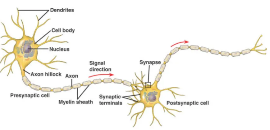
Figure 2.1: Elecotrochemical communication between two neurons. The left (presy-naptic) neuron generates an electric action potential (AP) that travels along its axon. Through the synpase, a chemical interneural connection, the signal contin-ues as postsynaptic potential (PSP) in the dendrites of the right neuron. Source:

http://www.kurzweilai.net/images/neuron_structure.jpg.

2.1

Introduction

Understanding the mechanisms underlying the functioning of the human brain remains a great challenge in modern neuroscience. Sophisticated non-invasive modalities capable of recording electromagnetic, metabolic, and hemodynamic changes related to neuronal activity have enabled large-scale studies on living human subjects. Despite the technological advances, non-invasiveness produces significant limitations regarding signal quality, tem-poral and spatial resolution, as well as information on single cell activity. Invasive techniques mostly used in animal experiments provide important complementary information. There has been growing interest in simultae-nous recordings with different modalities and studying how their underlying phenomena are related.

In this chapter, we focus on the electrophysiology of the brain and com-monly used recording modalities. We also briefly describe modalities ex-ploring the brain’s hemodynamics and metabolism and give examples for simultaneous multi-modal recordings. We then discuss current challenges concerning the signal analysis and outline some general goals for successful neuroelectic signal processing. These will serve as a guideline for the com-parison of existing techniques and the design of new methods in the following chapters. We conclude this chapter by discussing an exemplary multi-modal study in an animal model of epilepsy.

2.2

Electrophysiology of the brain

The human brain is estimated to contain around 100 billion neurons (Azevedo et al.,2009) which are permanently exchanging information along interneural

2.2. ELECTROPHYSIOLOGY OF THE BRAIN

Figure 2.2: Large assemblies of cortical pyramidal neurons generate electromagnetic fields of sufficient magnitudes to be measured on the scalp level. Left: Postsynaptic potentials (PSPs) travel along the apical dendrites of pyramidal cells in the cortex, directed perpendicular to the cortical surface. They generate primary (intracellular) and secondary (extracellular) currents. Center: Thanks to the parallel arrangement of the apical dendrites, the electromagnetic fields produced by a synchronously active neural assembly sum up. The accumulated field can be modeled as a dipole with normal orientation with respect to the cortical surface. Right: If the assembly is sufficiently large, the resulting electromagnetic cortical source can be detected at thescalp level.

Source: Baillet et al.(2001).

connections. This exchange is driven by electrochemical processes, through which neurons excite or inhibit other neurons to which they are connected through synapses, as depicted in Figure 2.1. When a neuron receives a large amount of excitatory signals in a short time interval, sufficient to sum above a certain threshold, the neuron fires: voltage-gated ion channels open, causing a transient depolarization in the neuron’s membrane. This so called action potential (AP) travels along the neuron’s axon and eventually contin-ues as a postsynaptic potential (PSP) in the dendrites of connected neurons. The respective potential differences cause primary currents to flow inside the cell. The electric circuit is closed by secondary currents through all parts of the surrounding volume conductor, including the entire brain, skull, and scalp. In addition, both primary and secondary currents cause a change in the magnetic field.

In theory, the generated potentials have an impact on the electromag-netism at all three levels: intracellular, extracellular inside the head, and on the surface of the skull (i.e., even outside the head in case of the magnetic field). However, the electromagnetic field generated by a single neuron is small and decays with the square of the distance to the field’s origin. Hence, it can only be empirically observed inside or in the immediate vicinity of the cell. In order to be measurable at the scalp level, the potentials of a synchronously firing neuron assembly need to add up.

Figure 2.3: First human EEG recorded in 1924 and published in Berger(1929). The actual recorded signal is shown on top, while the second is a sinusoidal reference signal of 10 Hz, demonstrating the oscillatory measurement to represent alpha rhythms (cf.

Section2.5).

The conditions for such an electromagnetic field superposition are prob-ably the most favorable for large assemblies of pyramidal cells in layers III and V of the cerebral cortex. These neurons have long apical dendrites per-pendicular to the cortical surface. Hence, when a large number of PSPs travel synchronously along the dendrites, the generated parallel electromag-netic fields add up. This process is shown in Figure 2.2. On the contrary, APs are believed to hardly contribute to the electromagnetic field at the scalp level. Although their relative membrane potential differences are larger (around 100 mV) than for PSPs (around 10 mV), they only last for several milliseconds (tens of milliseconds for PSPs). This makes the synchronicity constraint more stringent in order for APs to sum up.

More detailed information about the brain’s electrophysiology can be found inSpeckmann and Elger(2005).

2.3

Recording electromagnetic activity

2.3.1 Electroencephalography (EEG)

Ever since German physician Hans Berger obtained the first recordings of brain electrical activity in a human in 1924 (see Figure 2.3), electroen-cephalography (EEG) has been an extremely successful tool for studying the functioning of the brain. While Berger originally only used a single pair of electrodes to record potential differences between two locations on the scalp, a modern EEG protocol can measure up to 512 scalp potentials with sampling frequency of 10 000 Hz simultaneously. However, most setups only use less than 40 electrodes (see Figure 2.4). The equipment required for recording a modern EEG is simple and inexpensive, especially when com-pared to other brain imaging devices, and essentially consists of a set of electrodes, a signal amplifier, and a computer.

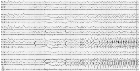
EEG almost instantaneously captures the electrical neural activity. This makes it the method of choice to study epilepsy, which is characterized by seizures involving abnormal electrical activity of neurons in the affected brain regions. A recording of such a seizure is shown in Figure2.5.

2.3. RECORDING ELECTROMAGNETIC ACTIVITY

Figure 2.4: Left: EEG recording session with multi-electrode cap at Inria Sophia

An-tipolis. Right: Visualtization of potential differences on the scalp, source: Vallagh´e

(2008).

The high temporal resolution around a millisecond provides a detailed temporal view of the brain activity. This furthermore allows direct real-time communication from the brain to an external device, known as brain-computer interface (BCI). These interfaces can help to study cognitive or sensory-motor functions and assist humans in the execution of these func-tions. A currently widely studied example is the P300 spelling device (cf. Section2.5.1), enabling text production solely through the EEG. Other ap-plications of EEG include the diagnosis of sleep disorders, encephalopathies, brain death, and the assessment of degrees of consciousness in coma.

In the past decades, much effort has been made to determine more pre-cisely the spatial locations of the active neural sources by exploiting the different electrode positions. However, despite improvements, the spatial resolution of EEG remains limited (around 20 mm), staying behind that of more recent brain imaging techniques, notably functional magnetic reso-nance imaging (fMRI). Another shortcoming of EEG is the generally high noise level in the recordings caused by neural background activity. This of-ten makes it necessary to acquire large amounts of data in order to extract useful information.

Nevertheless, EEG has hardly lost in popularity. Currently, much effort is made to maximize the usability of EEG devices through electrodes (or electrode caps) that do not require any conductive gel. These improvements could enable even more wide-spread use of EEG and the possibility of long-term monitoring outside clinics or laboratories.

2.3.2 Intracranial recordings

EEG usually refers to non-invasive recordings on the scalp. While these measurements outside of the head give a broad view of brain activity, their spatial resolution is limited. Different research studies and clinical applica-tions, however, require to record activity directly at precise locations in the

Figure 2.5: EEG recordings of a patient during epileptic seizure. The time series show potential differences between the two scalp electrodes marked on the left (e.g., Fp1-F3),

named according to standard placement conventions. Source: https://teddybrain.

wordpress.com.

brain by placing electrodes inside the skull.

In humans, the most common application of intracranial recordings is the exact localization of the cortical regions that generate epileptic seizures, often necessary prior to the treatment of epilepsy through surgery. For this purpose, single or multiple electrodes are either implanted directly onto the exposed surface of the cortex or even into deeper brain tissues. These techniques are known as electrocorticography (ECoG) and stereoelectroen-cephalography (sEEG), respectively.

In animals, intracranial recordings date back to as early as 1870 and are frequently used for research purposes. Depending on the size and impedance as well as the exact placement of the electrodes, neural activity can be mea-sured at micro- and mesoscopic levels. When placed close (within about 50 µm) to a neuron, a microelectrode can measure directly its unitary activ-ity (Harris et al.,2000). In contrast, larger electrodes that are located in a greater distance from the active sources will capture the combined activity of populations of neurons. The high frequency components above 300 Hz contain multiple-unit spike activity (MUA), while the signal filtered below 300 Hz is refered to as local field potential (LFP) (Logothetis,2003).

In order to investigate higher cognitive functions, animals with brain structures closest to humans such as non-human primates are prefered. How-ever, for the study of the basic neural mechanisms – for example for a better understanding of the origins and progress of epileptic seizures – smaller an-imals such as rats are frequently used.

2.3. RECORDING ELECTROMAGNETIC ACTIVITY

Figure 2.6: Left: A coronal slice through a human brain illustrating the cerebral cor-tex, that is, the brain’s outer layer. Its convoluted arrangement leads to ridges (gyri)

and fissures (sulci). Adapted from http://www.slideshare.net/kbteh/human-brain.

Right: The magnetic field resulting from an electric current dipole lies in a plane that

is perpendicular to the current flow. Source: Gramfort(2009).

2.3.3 Magnetoencephalography (MEG)

Magnetoelectroencephalography (MEG) is the counterpart to EEG, exploit-ing the magnetic field generated by the active neurons. Introduced in 1968 by physicist David Cohen (Cohen, 1968), MEG was able to record signals of quality similar to EEG only after the invention of the first SQUID (su-perconducting quantum interference device) detectors (Zimmerman et al.,

1970). In order to adequately measure the extremely small brain’s magnetic field in the order of 10-100 femtotesla (fT), modern MEG uses sophisticated equipment and requires a magnetically shielded room.

An advantage of MEG compared to EEG is the higher spatial resolution, due to typically larger numbers of detectors and the higher insensitivity of the magnetic field to skull and scalp. However, the complicated recording conditions and high equipment costs limit its use.

2.3.4 Complementary measurements of EEG and MEG

While electric potentials and the magnetic field measured outside of the head both originate from the electrical neural activity, there are important qualitative differences between EEG and MEG recordings. As explained in Section2.2, only large assemblies of simultaneously active pyramidal neurons are believed to significantly contribute to the electromagnetic field at scalp level. Since most electric current flows normally to the cortical surface, the direction of this field depends on the position of the source in the cortex, due to its convoluted arrangement in the brain (see Figure2.6). In cortical regions parallel to the skull (in particular the gyri), most current flows to the nearest parts of the skull and can thus be detected by EEG. The magnetic field lines, however, are located in a plane tangential to the skull, and the electric source will be hardly visible to MEG. Sources in a cortical sulcus, in turn, can be better observed through MEG than through EEG. Hence,

EEG and MEG are actually complementary in the sense that they are each optimal for differently located sources.

2.4

Recording metabolism and hemodynamics

The recording modalities presented in the previous section capture the neu-ral activity very directly, since the electromagnetic field propagates almost instantaneously. The greatest drawback is the limited spatial resolution of the non-invasive EEG and MEG.

Alternatively, neural activity can be measured indirectly through the brain’s metabolism and hemodynamics. Active brain regions require an in-creased supply of nutrients such as oxygen and glucose, which in turn results in a change of the cerebral blood flow (CBF). The metabolic and hemody-namic changes, however, typically occur with a time lag of 1 second or more after the neural events. Many different techniques are used to measure the metabolism or CBF, leading to very complementary observations compared to the electromagnetic recordings.

Functional magnetic resonance imaging (fMRI) uses the blood-oxygen-level dependent (BOLD) contrast to obtain detailed spatial maps of neural activation, with a resolution as fine as a few millimeters. Since the dis-covery of the BOLD-contrast by Seiji Ogawa in the 1990s (Ogawa et al.,

1990), the non-invasive fMRI has become the most widely-used tool for brain mapping research. The CBF and blood oxygenation can also be mea-sured through near-infrared spectroscopy (NIRS) (Gibson et al.,2005) which exploits the different optical absorption spectra of oxygenated and deoxy-genated hemoglobin. In contrast to fMRI, NIRS is more portable and can be used in infants. However, its use is limited to scan cortical tissue, whereas fMRI measures activity throughout the entire brain. Laser Doppler flowme-try (LDF), like NIRS, also involves the emission and detection of monochro-matic light to and from neural tissue. The frequency of the red or near-infrared light is shifted according to the Doppler principle when scattered back from moving blood cells. This allows to monitor changes in the CBF. As a drawback, LDF cannot be calibrated in absolute units, as noted in

Vongsavan and Matthews (1993). All three methods presented above are completely non-invasive.

In contrast, nuclear imaging, including positron emission tomography (PET) (Bailey et al.,2005) and single photon emission computed tomogra-phy (SPECT), require the injection of a radioactive tracer into the blood-stream. The tracer can be located as it produces measurable gamma rays either directly (SPECT) or indirectly through emitted positrons (PET). De-pending on the specific tracer, the recordings can measure either oxygen or glucose levels in the blood, or directly the CBF.

2.5. NEUROELECTRICAL SIGNALS

NIRS SPECT

ECoG/ sEEG

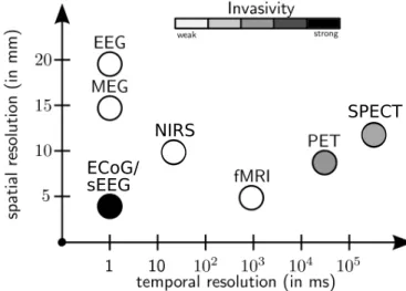
Figure 2.7: Comparison of spatial and temporal resolution of different brain imaging

techniques. Adapted fromOlivi(2011).

imaging techniques.

A comparison of the spatial and temporal resolution and the invasiveness of the presented electrophysiological and metabolic/hemodynamic recording modalities is shown in Figure2.7. We note that the presented selection is not exhaustive as their exist many other techniques for observing activity in the brain. Because of the complementary information obtained through hemo-dynamic and metabolic recordings compared to electromagnetic recordings, it has been of interest to combine two or more of these modalities for si-multaenous recordings. Such approaches can help to better understand the relationship between neural activity and blood flow changes, known as neu-rovascular coupling (Vanzetta et al.,2010).

2.5

Neuroelectrical signals

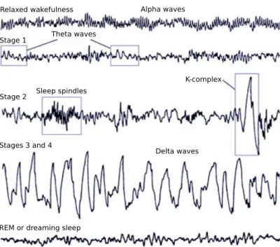
Neuroelectrical recordings can produce signals with very different character-istics. The first measured EEGs by Hans Berger showed strong oscillatory activity around 10 Hz. Oscillations of different frequencies have since been observed and divided into distinct frequency bands, associated with differ-ent types of mdiffer-ental activity: delta rhythm (< 4 Hz, e.g., deep sleep), theta rhythm (4 − 7 Hz, e.g., drowsiness), alpha rhythm (8 − 13 Hz, e.g., relaxed, eyes closed), beta rhythm (14 − 30 Hz, e.g., active thinking, certain sleep stages), and gamma rhythm (> 30 Hz, e.g., active information processing); see, for instance,S¨ornmo and Laguna(2005, chapter 2). Other than rhyth-mic activity, transient waveforms such as increases or decreases in the electric potential are observed. Different types of rhythmic and transient activity are also observed during different sleep stages (see Figure2.9).