HAL Id: hal-03051981
https://hal.archives-ouvertes.fr/hal-03051981
Submitted on 10 Dec 2020
HAL is a multi-disciplinary open access
archive for the deposit and dissemination of
sci-entific research documents, whether they are
pub-lished or not. The documents may come from
teaching and research institutions in France or
abroad, or from public or private research centers.
L’archive ouverte pluridisciplinaire HAL, est
destinée au dépôt et à la diffusion de documents
scientifiques de niveau recherche, publiés ou non,
émanant des établissements d’enseignement et de
recherche français ou étrangers, des laboratoires
publics ou privés.
Acetone variability in the upper troposphere: analysis of
CARIBIC observations and LMDz-INCA
chemistry-climate model simulations
T. Elias, S. Szopa, A. Zahn, T. Schuck, C. Brenninkmeijer, D. Sprung, F.
Slemr
To cite this version:
T. Elias, S. Szopa, A. Zahn, T. Schuck, C. Brenninkmeijer, et al.. Acetone variability in the upper
troposphere: analysis of CARIBIC observations and LMDz-INCA chemistry-climate model
simula-tions. Atmospheric Chemistry and Physics, European Geosciences Union, 2011, 11 (15), pp.8053-8074.
�10.5194/ACP-11-8053-2011�. �hal-03051981�
www.atmos-chem-phys.net/11/8053/2011/ doi:10.5194/acp-11-8053-2011
© Author(s) 2011. CC Attribution 3.0 License.
Atmospheric
Chemistry
and Physics
Acetone variability in the upper troposphere: analysis of CARIBIC
observations and LMDz-INCA chemistry-climate model simulations
T. Elias1,*,**, S. Szopa1, A. Zahn3, T. Schuck2, C. Brenninkmeijer2, D. Sprung3, and F. Slemr2
1Laboratoire des Sciences du Climat et de l’Environnement/CEA-CNRS-UVSQ-IPSL, UMR8212, L’Orme des Merisiers, 91191 Gif-sur-Yvette, France
2Atmospheric Chemistry Division, Max Planck Institute for Chemistry, Mainz, Germany
3Institute of Meteorology and Climate Research, Karlsruhe Institute of Technology (KIT), Germany *now at: HYGEOS, Euratechnolgies, 165, Avenue de Bretagne, 59000 Lille, France
**now at: Honorary research associate at CRG, GAES, University of the Witwatersrand, Johannesburg, South Africa Received: 22 December 2010 – Published in Atmos. Chem. Phys. Discuss.: 17 March 2011
Revised: 10 July 2011 – Accepted: 19 July 2011 – Published: 8 August 2011
Abstract. This paper investigates the acetone variabil-ity in the upper troposphere (UT) as sampled during the CARIBIC airborne experiment and simulated by the LMDz-INCA global chemistry climate model. The aim is to (1) de-scribe spatial distribution and temporal variability of acetone; (2) propose benchmarks deduced from the observed data set; and (3) investigate the representativeness of the observational data set.
According to the model results, South Asia (including part of the Indian Ocean, all of India, China, and the Indochi-nese peninsula) and Europe (including Mediterranean Sea) are net source regions of acetone, where nearly 25 % of North Hemispheric (NH) primary emissions and nearly 40 % of the NH chemical production of acetone take place. The im-pact of these net source regions on continental upper tro-pospheric acetone is studied by analysing CARIBIC obser-vations of 2006 and 2007 when most flight routes stretched between Frankfurt (Germany) and Manila (Philippines), and by focussing over 3 sub-regions where acetone variability is strong: Europe-Mediterranean, Central South China and South China Sea.
Important spatial variability was observed over different scales: (1) east-west positive gradient of annually averaged acetone vmr in UT over the Eurasian continent, namely a factor two increase from east to west; (2) ocean/continent contrast with 50 % enhancement over the continents; (3) the
Correspondence to: T. Elias
(te@hygeos.com)
acetone volume mixing ration (vmr) may vary in summer by more than 1000 pptv within only 5 latitulongitude de-grees; (4) the standard deviation for measurements acquired during a short flight sequence over a sub-region may reach 40 %. Temporal variability is also important: (1) the ace-tone volume mixing ratio (vmr) in the UT varies with the season, increasing from winter to summer by a factor 2 to 4; (2) a difference as large as 200 pptv may be observed be-tween successive inbound and outbound flights over the same sub-region due to different flight specifications (trajectory in relation to the plume, time of day).
A satisfactory agreement for the abundance of acetone is found between model results and observations, with e.g. only 30 % overestimation of the annual average over Central-South China and the Central-South China Sea (between 450 and 600 pptv), and an underestimation by less than 20 % over Europe-Mediterranean (around 800 pptv). Consequently, an-nual budget terms could be computed with LMDz-INCA, yielding a global atmospheric burden of 7.2 Tg acetone, a 127 Tg yr−1global source/sink strength, and a 21-day mean residence time.
Moreover the study shows that LMDz-INCA can repro-duce the impact of summer convection over China when boundary layer compounds are lifted to cruise altitude of 10– 11 km and higher. The consequent enhancement of acetone vmr during summer is reproduced by LMDz-INCA, to reach agreement on an observed maximum of 970 ± 400 pptv (av-erage during each flight sequence over the defined zone ± standard deviation). The summer enhancement of acetone is characterized by a high spatial and temporal heterogeneity,
showing the necessity to increase the airborne measurement frequency over Central-South China and the South China Sea in August and September, when the annual maximum is expected (daily average model values reaching potentially 3000 pptv). In contrast, the annual cycle in the UT over Europe-Mediterranean is not reproduced by LMDz-INCA, in particular the observed summer enhancement of acetone to 1400 ± 400 pptv after long-range transport of free tropo-spheric air masses over North Atlantic Ocean is not repro-duced. In view of the agreement on the acetone annual cy-cle at surface level, this disagreement in UT over Europe in-dicates misrepresentation of simulated transport of primary acetone or biased spatial distribution of acetone chemical sinks and secondary sources. The sink and source budget in long-range transported free tropospheric air masses may be studied by analysing atmospheric chemical composition ob-served by CARIBIC in summer flights between North Amer-ica and Europe.
1 Introduction
Hydroxyl (OH) and hydroperoxy radical (HO2) dominate background tropospheric chemistry through their oxidative roles. In fact, the oxidation of CO and hydrocarbons is the main source of tropospheric ozone (Brasseur et al., 1999). Water vapour is the main precursor of primary tropospheric OH, except in the upper troposphere (UT) where dry condi-tions prevail. Here acetone (CH3COCH3)becomes a candi-date as the main source of OH (Singh et al., 1995). Indeed, Wennberg et al. (1998) could reach near agreement between measured and simulated OH concentration in the UT by con-sidering 300 pptv acetone in a photochemical box model, un-der specific conditions. For example, OH production is more sensitive to acetone at low solar zenith angle, and differences reaching a factor 5 are still observed. The significance of ace-tone was later confirmed using Chemistry-Climate Models: for example Folberth et al. (2006) showed using the LMDz-INCA model, that acetone and methanol play a significant role in the upper troposphere/lower stratosphere budget of peroxy radicals, with an increase in OH and HOx concentra-tions of 10 to 15 % being attributed to acetone. Chatfield et al. (1987) noted that acetone can be considered an indicator of properly modelled atmospheric chemistry in the UT, for instance as a tracer of previous photochemical activity in an air parcel.
It is currently accepted that the sources of acetone consist mostly of primary terrestrial biogenic and oceanic emissions, complemented by secondary chemical production, with sinks by photolysis, oxidation, and a substantial degree of mostly dry deposition over land and oceans. Nevertheless, uncer-tainties remain in the acetone budget. For example, Jacob et al. (2002) improved the agreement between model and observational data by (1) adding an oceanic source, (2)
in-creasing the terrestrial vegetation contribution, and (3) de-creasing the contribution from vegetation decay. In line with the fairly recent revision of the acetone photolysis quantum yield in terms of a temperature dependent function (Blitz et al., 2004), Arnold et al. (2005) estimated a reduced pho-tolysis sink. Marandino et al. (2006) proposed to compen-sate for this by increasing the ocean sink in order to ac-commodate results of air/sea flux measurements over the Pacific Ocean. Consequently, for total source/sink strength of around 100 Tg yr−1, estimates of the oceanic contribu-tion currently range between a net source of 13 Tg yr−1 (Ja-cob et al., 2002) and a net sink of 33 Tg yr−1(Marandino et al., 2006). Concerning primary terrestrial biogenic emission, Potter et al. (2003) proposed a wide range of source strengths between 54 and 172 Tg yr−1for terrestrial vegetation and be-tween 7 and 22 Tg yr−1for plant decay.
Most recent budget studies have relied on data compiled by Emmons et al. (2000): (1) the ocean source was taken into account for improving agreement over the Pacific Ocean (Jacob et al., 2002; Folberth et al., 2006); (2) the terres-trial biogenic primary emissions were modified to fit lower tropospheric observations (Jacob et al., 2002); (3) the ace-tone photolysis quantum yield (with its strong impact in the UT; Arnold et al., 2004) was changed to improve agreement for the vertical column (Arnold et al., 2005), especially over the Pacific Ocean. This all shows the problem of resolving the acetone budget, which by its variability adds an addi-tional challenge. Because aircraft measurements during field campaigns are essentially “snapshots”, Emmons et al. (2000) claim that their data composite can not be regarded as clima-tology. Observation-based constraints need to be more com-plete to become applicable to all modelled source, sink and transport processes. In particular, few measurements were hitherto available in the northern mid-latitude and over con-tinents, and temporal variability in the UT has been sounded only sporadically.
The “civil aircraft” approach of the CARIBIC experiment (Civil Aircraft for Regular Investigation of the atmosphere Based on an Instrument Container) (Brenninkmeijer et al., 2007) and other projects such as MOZAIC (e.g. Marenco et al., 1998; Thouret et al., 2006) and CONTRAIL (Machida et al., 2008) provide an opportunity to more systematically sample the annual cycle and the inter-annual variability of main atmospheric trace gases on a large scale. CARIBIC, with its extensive instrument payload is suitable to help to address the acetone budget issue. Sprung and Zahn (2010) compiled three years of CARIBIC data to derive the acetone distribution around the tropopause north of 33◦N, showing
that acetone volume mixing ratio (vmr) varies by a factor of four with season.
The purpose of our work is to scrutinize model results and observations for (1) describing spatial distribution and tem-poral variability of acetone in the UT; (2) proposing bench-marks deduced from the observation data set; and (3) inves-tigating the representativeness of the observational data set.
The simulation results are provided by LMDz-INCA, which integrates a comprehensive representation of the photochem-istry of methane and volatile organic compounds from bio-genic, anthropobio-genic, and biomass-burning sources (Fol-berth et al., 2006). The CARIBIC experiment provides the acetone measurements in the UT mainly over NH continen-tal regions where major sources are located and where chem-ical activity significantly contributes to acetone sources and sinks. Main flight routes for the period considered extend between Frankfurt (Germany) and Manila (Philippines), also providing the opportunity to study the impact of rapid uplift-ing of pollutants over China and the South China Sea.
The LMDz-INCA model and the CARIBIC experiment are described in Sects. 2 and 3 respectively, together with the method used to compare the two data sets. Budget terms on global and regional scales are also provided in Sect. 2. Results of comparisons are discussed in Sect. 4. The focus is on the UT over South-Central China and the South China Sea, with impacts of pollution events, and over the Europe-Mediterranean region affected by long-range transport over the North Atlantic Ocean. Measurements of O3and CO are also used to discuss the chemical signature of air masses, with the help of computed back-trajectories.
2 Global budget of acetone according to LMDz-INCA 2.1 The LMDz-INCA set-up
LMDz-INCA consists of the INteraction Chemistry-Aerosols (INCA) module representing tropospheric chem-istry, coupled with the Global Circulation Model LMDz (Hourdin et al., 2006). Fundamentals are presented by Hauglustaine et al. (2004) and first results with the full tro-pospheric chemistry are presented by Folberth et al. (2006). This model is commonly used in international multi-model experiments to investigate climate-chemistry issues or inter-continental transport (e.g. Sanderson et al., 2008; Fiore et al., 2009). Large scale advection is nudged using ECMWF re-analysis data. Global tropospheric fields of greenhouse gases (CO2, CH4, O3, N20), aerosols, water vapour and non-methane hydrocarbons are simulated on a horizontal grid, improved since Folberth et al. (2006), from 3.75◦ longi-tude × 2.5◦ latitude to 3.75◦×1.875◦ spatial resolution in the LMDz4-INCA3 version used here. The number of re-active species in INCA has been increased from 83 (of which 58 are transported) to 89. Currently 43 photolytic, 217 thermo-chemical and 4 heterogeneous reactions are inte-grated in the INCA module. In particular, acetone is directly involved in 21 reactions, e.g. in oxidation of alkenes, alka-nes, alpha pinealka-nes, and photolysis. The quantum yield for acetone photolysis is updated in LMDz4-INCA3, according to Blitz et al. (2004).
Primary biogenic emissions of isoprene, terpenes, methanol, and acetone are prepared by the global
vegeta-tion model ORCHIDEE (ORganizing Carbon and Hydrol-ogy In Dynamic EcosystEms; Krinner et al., 2005), as de-scribed in Lathi`ere et al. (2006). Primary emission of ace-tone by biomass burning is taken from van der Werf et al. (2006) (GFED-v2). The anthropogenic contribution is based on the EDGAR v3.2 emission database (Olivier and Berdowski, 2001), except that for non-methane volatile or-ganic compounds, which is based on the EDGAR v2.0 emis-sion database (Olivier et al., 1996). The ocean source is de-rived from Jacob et al. (2002). GCM primitive equations are resolved by LMDz every 3 min, the large scale transport has a time step of 15 min, and physical processes of 30 min. INCA computes primary emissions, deposition and chemical equa-tions every 30 min.
Folberth et al. (2006) compared volatile organic com-pound fields simulated by the NMHC1.0 model version with field campaign results presented by Emmons et al. (2000) and Singh et al. (2001). Their simulated values have been sampled from the model output over the same regions and months as the airborne observational data: western North At-lantic Ocean in summer, eastern North AtAt-lantic Ocean and tropical Atlantic Ocean in early autumn, East Asian coasts in winter, Pacific Ocean in early spring. Folberth et al. (2006) show a satisfactory overall agreement, with more frequent overestimation than underestimation. CARIBIC now allows us to extend the available data set to continents and to inves-tigate the seasonal variability (Sect. 3).
2.2 Budget terms
2.2.1 Global budget, sources and sinks
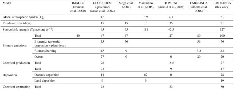
The budget terms computed with LMDz-INCA are presented in Table 1 together with literature results. Annual cycles of the global budget terms are shown in Fig. 1. Since no inter-annual trend is simulated for the inter-annual global acetone bur-den, 2007 is used as reference for budget analyses. The to-tal source in LMDz-INCA is apportioned as 60 % primary terrestrial biogenic, 16 % primary oceanic, and 20 % sec-ondary chemical production, providing total source strength of 127 Tg yr−1, which exceeds previous estimates. Indeed primary emissions are larger by 50 % than considered by Ja-cob et al. (2002), and by 25 % than Singh et al. (2004) and Folberth et al. (2006) (Table 1). The ocean source remains constant at 20 Tg yr−1 since Folberth et al. (2006), but the primary terrestrial biogenic contribution increased from 56 to 76 Tg yr−1since Folberth et al. (2006), in close agreement with 66–71 Tg yr−1presented by Lathi`ere et al. (2006). This is at the lowest range estimated by Potter et al. (2003) of 61– 194 Tg yr−1for biogenic emission (terrestrial vegetation and plant decay). Chemical production of 27 Tg yr−1of acetone estimated by LMDz-INCA is similar to estimates by Jacob et al. (2002). No values on chemical production were reported by Folberth et al. (2006).
Table 1. LMDz-INCA computation of acetone global budget terms, as well as literature results. Sources correspond to primary emission
and chemical production, sinks correspond to deposition and chemical destruction. Primary emission and deposition are further apportioned according to continental/oceanic contributions.
Model IMAGES GEOS-CHEM Singh et al. Marandino TOMCAT LMDz-INCA LMDz-INCA (Emmons a posteriori (2004) et al. (2006) (Arnold et al., 2005) (Folberth et al., (this work) et al., 2000) (Jacob et al., 2002) 2006)
Global atmospheric burden (Tg) 3.8 3.9 4.1 7.2
Residence time (days) 15 15 13 35 21
Source/sink strength (Tg acetone yr−1) 95 95 111 42.5 127
Primary emissions
Total 40 67 67 27 80 100
Biogenic: terrestrial vegetation + plant decay
35 56 56 76
Biomass burning 4.5 9 3.2 2.4
Ocean 27 0 0 20 20
Chemical production Total 28 15.5 27
Deposition
Total 23 9 47
Oceanic deposition 14 62 0 28
Land deposition 9 9 19
Chemical destruction Total 73 33 80
One third of the acetone load is deposited (mainly dry de-position), and two thirds is either oxidised or photolysed. Chemical destruction is similar to simulations by Jacob et al. (2002), but deposition computed by LMDz-INCA is in-creased to reach equilibrium of equal global source and sink strengths. The chemical budget by LMDz-INCA displays a net chemical sink of 53 Tg yr−1on a global scale (similar to 45 Tg yr−1estimated by Jacob et al., 2002). The oceans are a net sink of 8 Tg yr−1, resulting from 20 Tg yr−1emissions and 28 Tg yr−1deposition.
The mean residence time of 21 days is within the range in-ferred from previous studies (Table 1). However, similarly to the acetone source strength, our estimated atmospheric bur-den of 7.2 Tg is larger than previous estimates by Jacob et al. (2002), Arnold et al. (2005), and Marandino et al. (2006). An exact balance between source and sink is not constantly found, causing a small seasonal variability of the global at-mospheric burden of acetone. Annual cycles of the global source and sink terms are shown in Fig. 1a. Maxima of the source terms occur during boreal summer, revealing the sig-nature of the dominant biogenic source. Because the main acetone source is terrestrial, a contrast is simulated between the northern and southern hemisphere, with more acetone strength and burden in the NH, and with more intense an-nual cycles, while the residence time of 21 days is equal in both hemispheres.
On a global scale, minima of the budget terms are found in boreal winter and maxima in boreal summer. The global budget is annually balanced, but on a monthly basis accumu-lation of acetone occurs in July at a rate of 0.7 Tg month−1. Depletion occurs in December at a rate of −0.2 Tg month−1. Taking into account the acetone residence time, the annual
cycle of the atmospheric burden is delayed by one or two months, with a minimum of 6.4 Tg in February and a maxi-mum of 8.1 Tg in September/October.
2.2.2 Regional features
Budget terms were computed for continental regions enclos-ing main route sections taken by the CARIBIC experiment in 2006–2007, namely South Asia and Europe (Sect. 3). South Asia extends between 10◦ and 40◦N latitude and between 20◦and 130◦E longitude, Europe extends between 30◦and 70◦N and between 10◦W and 50◦E. The respective budget terms proportioned to those regions and monthly averages of the regional budget terms are plotted in Fig. 1b and c. Due to its sufficiently long residence time, long range transport smoothes the spatial distribution of the acetone burden com-puted on an annual basis, despite high spatial heterogeneity observed in the source pattern.
South Asia is a net source region, with 2 Tg yr−1 excess net production (around 15 % of the regional source strength of 13 Tg yr−1), which is transported to other regions of the world, as on an annual basis, the atmospheric burden of ace-tone (0.48 Tg aceace-tone) is proportional to the covered surface area (11 %). Regarding geographical differences, sources and sinks are proportionally larger over South Asia than on a hemispheric scale, with primary emission, deposition and chemical loss representing around 15 % of the NH terms, and the chemical production representing up to 23 % (with 4.8 Tg yr−1). The chemical production, in excess relatively to the other terms, may account entirely for the excess net production of acetone in South Asia. The annual cycles of the regional budget terms are similar to that of the global
T. Elias et al.: Acetone variability in the upper troposphere 8057
Figures
(a)
(b)
(c)
Figure 1. Annual cycle of the acetone budget terms (in Tg/month), computed by LMDz-INCA for (a) the world, (b) South Asia, and (c) Europe. The net budget is computed as source - sink. Sources are divided into primary emission, and chemical production, and sinks (counted negatively) into dry deposition and chemical loss.
Fig. 1. Annual cycle of the acetone budget terms (in Tg month−1), computed by LMDz-INCA for (a) the world, (b) South Asia, and
(c) Europe. The net budget is computed as source-sink. Sources are
divided into primary emission, and chemical production, and sinks (counted negatively) into dry deposition and chemical loss.
annual cycle in terms of seasonal minimum and maximum (Fig. 1b and c). However the annual cycles have larger am-plitudes with primary production increasing by a factor 2.3 and chemical loss by a factor three. The net production in the region exhibits a strong annual cycle, changing by a fac-tor 4 with the season.
As for South Asia, the atmospheric burden of acetone over Europe is proportional to the surface area covered by the re-gion (8 % with 0.35 Tg acetone) while the European rere-gion also provides excess acetone during all seasons cumulating to +1.7 Tg yr−1 (around 25 % of the regional source strength of 6.8 Tg yr−1). Concomitantly, the annual chemical production is important over Europe, reaching 13 % of the NH chemical production (which represents 8 % of the NH surface area), and even exceeds primary emission (representing 8 % the NH primary emission) during the winter (Fig. 1c). This excess regional chemical production combined with a deficit in sim-ulated regional chemical loss (accounting for only 6 % of the NH chemical loss), almost results in net regional chemical balance: from a net chemical sink of 0.2 Tg month−1in sum-mer, reversing to a net chemical source of 0.1 Tg month−1in winter, while on a global scale there is always a net chemical sink. A strong seasonal cycle is also simulated for primary production, with a factor eight change with season. Depo-sition appears to be important over the European region as its magnitude is similar to chemical loss, and even exceeds chemical loss in winter, which is inferred neither for South Asia nor on a global scale.
Because primary emissions and dry deposition occur ex-clusively at surface level, the only source/sink terms impact-ing the vertical profile of the global budget are the chemical terms. Because the chemical budget results in a net sink on a global scale, the atmosphere is expected to be a sink for ace-tone. Consequently, the lowermost atmospheric layers are simulated to be net source, with an overlaying net chemi-cal sink, all through the year. Over Europe, the net acetone sink at 238 hPa can reach 500 Mg yr−1and 100 Mg month−1 in August, and over South Asia it may reach 1500 Mg yr−1 and 200 Mg month−1 in August. Consequently, plumes of acetone at such altitude can only be observed thanks to trans-port of primary and secondary acetone from the boundary layer. The two net source regions Europe and South Asia will be discussed in Sect. 4, in terms of acetone content in the UT, as they are locations where most data is acquired by the CARIBIC experiment.
3 The strategy for comparing model data with CARIBIC measurements
3.1 CARIBIC data set
The CARIBIC project (http://www.caribic-atmospheric. com/) provides measurements of acetone volume mixing ratio (vmr) by an instrumented airfreight container oper-ated during Lufthansa’s regular long-distance flights (Bren-ninkmeijer et al., 2007). Four consecutive intercontinen-tal flights are made almost monthly, thus covering around 400 000 km annually. Acquisition is performed during all seasons, for a large range of solar insolation conditions, and along four main routes. In 2006 and 2007, most flights were to Manila, with two flights to South America (February
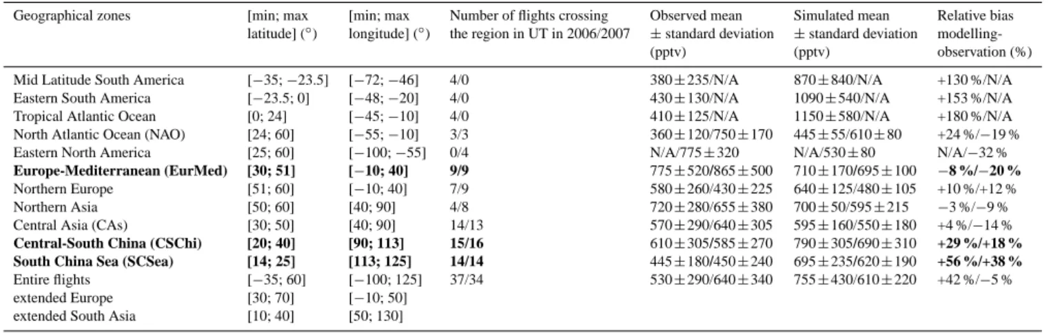
Table 2. Average and standard deviation are computed for all 2006 and 2007 flight segments included between the minimum and maximum
longitude and latitude of the 11 geographical zones, exclusively in the troposphere, for co-located modelling results and observation. Standard deviation represents here the temporal and spatial variability. Number of flights crossing the geographical zones is also given for each year. Computations are similarly made for entire flights, independently the location. Coordinates are also given for the two extended geographical regions (Europe and South Asia), where budget terms are computed in Sect. 2. Bias is computed as observation subtracted from modelling results, divided by observation. Focus regions are showed in bold face.
Geographical zones [min; max [min; max Number of flights crossing Observed mean Simulated mean Relative bias latitude] (◦) longitude] (◦) the region in UT in 2006/2007 ±standard deviation ±standard deviation
modelling-(pptv) (pptv) observation (%) Mid Latitude South America [−35; −23.5] [−72; −46] 4/0 380 ± 235/N/A 870 ± 840/N/A +130 %/N/A Eastern South America [−23.5; 0] [−48; −20] 4/0 430 ± 130/N/A 1090 ± 540/N/A +153 %/N/A Tropical Atlantic Ocean [0; 24] [−45; −10] 4/0 410 ± 125/N/A 1150 ± 580/N/A +180 %/N/A North Atlantic Ocean (NAO) [24; 60] [−55; −10] 3/3 360 ± 120/750 ± 170 445 ± 55/610 ± 80 +24 %/−19 % Eastern North America [25; 60] [−100; −55] 0/4 N/A/775 ± 320 N/A/530 ± 80 N/A/−32 %
Europe-Mediterranean (EurMed) [30; 51] [−10; 40] 9/9 775 ± 520/865 ± 500 710 ± 170/695 ± 100 −8 %/−20 %
Northern Europe [51; 60] [−10; 40] 7/9 580 ± 260/430 ± 225 640 ± 125/480 ± 105 +10 %/+12 % Northern Asia [50; 60] [40; 90] 4/8 720 ± 280/655 ± 380 700 ± 50/595 ± 215 −3 %/−9 % Central Asia (CAs) [30; 50] [40; 90] 14/13 570 ± 290/640 ± 305 595 ± 160/550 ± 180 +4 %/−14 %
Central-South China (CSChi) [20; 40] [90; 113] 15/16 610 ± 305/585 ± 270 790 ± 305/690 ± 310 +29 %/+18 % South China Sea (SCSea) [14; 25] [113; 125] 14/14 445 ± 180/450 ± 240 695 ± 235/620 ± 190 +56 %/+38 %
Entire flights [−35; 60] [−100; 125] 37/34 530 ± 290/640 ± 340 755 ± 430/610 ± 220 +42 %/−5 % extended Europe [30; 70] [−10; 50]
extended South Asia [10; 40] [50; 130]
and March 2006), and two to North America (September 2007). The measurement technique using a Proton-Transfer-Reaction quadrupole Mass Spectrometer was described by Sprung and Zahn (2010). The total uncertainty of the acetone data is ∼10 % above 200 pptv and ∼20 pptv below 200 pptv. With a 1-min temporal resolution, approximately 10 000 val-ues are available each year. The CARIBIC data set presented highly variable acetone values due to different sampled air masses (K¨oppe et al., 2009), season, and aircraft position rel-atively to the tropopause (Sprung and Zahn, 2010), and due to pollution events (Lai et al., 2010). First we briefly sum-marise some key results from these studies.
K¨oppe et al. (2009) identified five air mass types using cluster analysis applied to a data set composed of mixing ratios of cloud water, water vapour, O3, CO, acetone, ace-tonitrile, NOy and for aerosol number densities, measured exclusively on flights to Guangzhou and Manila in 2006 and 2007. The cluster analysis could not be applied if one or more measured parameters were missing. Consequently, due to incidental instrument failure and calibration intervals, air mass characteristics could be identified for only one third of all acquisitions (K¨oppe et al., 2009). Acetone vmr seems to be related with the air mass origin: e.g. acetone vmr in sum-mer was 780 pptv (±33 % standard deviation) in the cluster representing high clouds (HC) and was 1230 pptv (±31 %) in free troposphere (FT) air masses (K¨oppe et al., 2009). The seasonal dependence of acetone vmr depends on the air mass: it was strong in FT air masses where acetone vmr increased by a factor of two from winter to summer, and it was less im-portant in boundary layer air mass (BL), where acetone vmr changed by only 30 %.
Sprung and Zahn (2010) discriminated tropospheric data from stratospheric data, and also defined a (mixing-based) height above the thermal tropopause, by translating ozone concentrations measured in flight, using data collected at 12 ozonesonde stations. Data was acquired by CARIBIC mostly in the troposphere (76 % in 2006, 64 % in 2007). The loca-tion of sampling relative to the tropopause was decisive as the averaged acetone vmr in 2006 was 530±290 pptv in the up-per troposphere and 350 ± 250 pptv in the lowermost strato-sphere. Acetone decreased further down to 230 ± 150 pptv 0.5 km above the tropopause. Strong seasonality was ob-served north of 33◦N, where a maximum of ∼900 pptv was observed in summer and lowest values of ∼200 pptv in win-ter at the tropopause (Sprung and Zahn, 2010). The air mass identification techniques by K¨oppe et al. (2009) and Sprung and Zahn (2010) are complementarily used in this paper.
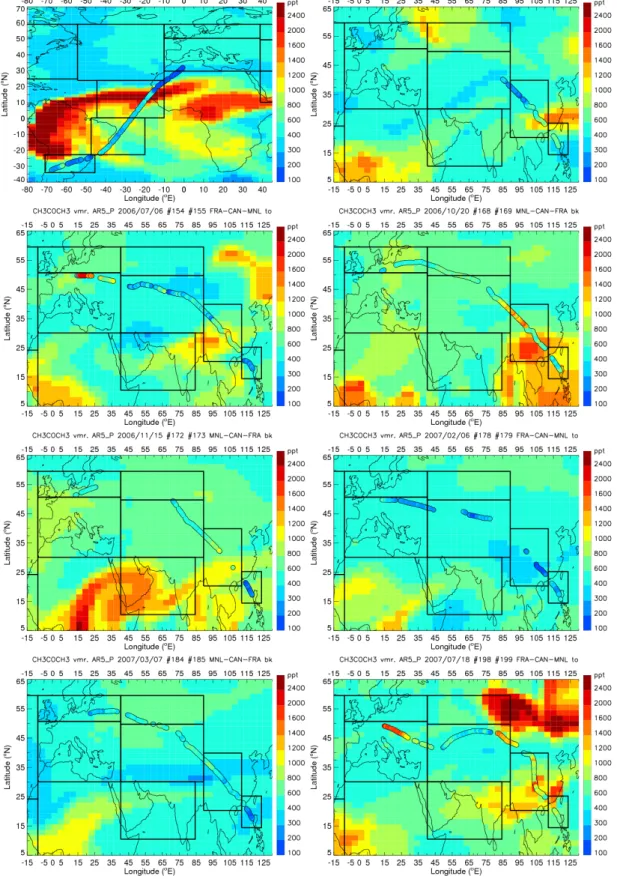
The CARIBIC data set shows large spatial and temporal variability in acetone vmr measured in the upper troposphere. This is illustrated in Fig. 2, which displays acetone vmr from several flights with values between 100 and 2600 pptv. The annual maximum acetone concentration in the UT was observed over Germany in July 2006, just after the ascent from Frankfurt airport: acetone varied between 1200 and 2600 pptv along 50◦N latitude, from 15 to 22◦E (Fig. 2)
at a constant altitude of 280 hPa. The 2007 maximum was observed in August over eastern Kazakhstan during a flight from Guangzhou to Frankfurt: acetone varied between 1000 and 2200 pptv along 50◦latitude between 50 and 60◦ longi-tude, at 240 hPa. Globally, maximal values in August 2003 were found to reach 3000 pptv between 300 and 500 hPa and to reach 2000 pptv above 200 hPa (Moore et al., 2010).
Fig. 2. Acetone vmr (pptv) along the flight track, acquired onboard the CARIBIC passenger aircraft for several flights in 2006 and 2007,
Figure 2. Acetone vmr (pptv) acquired onboard the passenger aircraft along the flight track
for several flights, superimposed on maps of daily averaged simulated acetone vmr at 238 hPa
Fig. 2. Continued.
Lai et al. (2010) showed the impact on acetone vmr of pol-lution events observed in the UT in April 2007. Polluted air masses crossing the flight trajectory over China led to en-hancements from 350 to 1800 pptv for acetone, from 70 to 150 ppbv for CO with O3remaining below 100 ppbv. Back trajectories located the air mass origin over the Indochinese Peninsula, bringing pollution from biomass/biofuel burning activities (Lai et al., 2010).
3.2 Methodology to compare observed data to model results
In this paper, besides the 2006 and 2007 routes to Asia, routes to the Americas are used for comparison, thus extending the
latitude to span 30◦S to 55◦N. Model results are co-located
to observations to allow comparison. Simulated values of acetone are spatially (vertically and horizontally) and tem-porally interpolated along the flight tracks, at the coordinates (time and space) of each data acquisition event.
To ensure consistency in the data set, small-scale variabil-ity due to changes in acquisition altitude are avoided by only using measurements when the aircraft cruises at constant al-titude, i.e. when altitude difference between two successive acquisitions made in 1 min is smaller than 1 hPa. Conse-quently, the data set is mostly composed of measurements acquired at cruising altitudes above 300 hPa. Around 70 % of the measurements were acquired at altitudes between 200 and 250 hPa and 25 % at altitudes between 250 and 300 hPa.
Because the INCA module resolves only tropospheric chemistry, the height above the tropopause defined by Sprung and Zahn (2010) is used to remove measurements acquired in the stratosphere. As measurement frequency in the strato-sphere increases with latitude, most data acquired over north-ern Asia are screened out. The data set is then composed of 7500 observed values in 2006 and 6100 values in 2007. Most values (around 60 %) of acetone fall between 200 and 600 pptv. All air masses identified as lowermost stratosphere by K¨oppe et al. (2009) are consistently localised in the strato-sphere according to Sprung and Zahn (2010). Conversely, all summer HC and winter FT and BL cluster samples are tropo-spheric. For 2006 and 2007, tropospheric air mass character-istics are identified for only 3400 data points. Moreover, as most flights started and finished in Frankfurt at night, mea-surements were chiefly made during the night (55 % in 2007, 68 % in 2006).
We define 11 geographical zones along all flight routes (Table 2) to compute regional averages of acetone vmr (one value per region and per flight), with the standard deviation as an indication of the spatial variability (the temporal vari-ability of acetone is negligible in the few hours necessary to cross the zone). This approach is used for co-located simula-tion and measurement data sets. The annual cycle of acetone is illustrated by plotting time series of zonal averages, which are analysed in the subsequent sections. During each round trip, given that the aircraft takes similar routes in both di-rections, it usually crosses a given zone twice within 24 h. Consequently, the time series for a year show commonly two points per month, reflecting short term temporal variability.
We are also interested in examining the possible effects of irregularities in the CARIBIC sampling on properly repre-senting the annual cycle. For that purpose co-located simu-lation and measurement averages are compared to averaged vmr simulated at constant altitude of 238 hPa, over the full zone for the whole month, hereafter referred to as the cli-matological value. Also considered is how well spatial vari-ability is represented by the standard deviations over all grid boxes of the different zones, as discussed in the subsequent sections.
4 Comparison of results
4.1 Impact of air mass history on geographical variability
Annual averages of measurements and co-located model re-sults for each zone are presented in Table 2. It shows that the magnitude of acetone vmr in UT can be reproduced by LMDz-INCA, but disagreements occur as a function of geo-graphical location. Averaging the whole data set (7500 data points in 2006, and 6100 in 2007) provides a mean ace-tone value of 530 ± 290 pptv observed in the UT in 2006 and 640 ± 340 pptv in 2007. Bearing in mind the high
stan-dard deviation as a result of significant temporal and spa-tial variability of acetone along the flight tracks, there is a satisfactory agreement with simulations (Table 2). Acetone vmr generally appears to be larger over the continents than over the oceans. The largest observed averages are encoun-tered over the EurMed region, of 770 ± 520 pptv in 2006 and 860 ± 500 pptv in 2007, with large standard deviation sug-gesting strong temporal variability. The smallest averages below 500 pptv are observed: (1) over the Atlantic Ocean and South America in only one season (February–March 2006); (2) over the South China Sea in 2006 and 2007, but with large standard deviation (around 50 %) due to measurements extending over several seasons. Averages over the North At-lantic Ocean (NAO) may give an indication of the seasonal impact: acetone doubles from winter 2006 to summer 2007.
Overall agreement is observed within ±30 % in most re-gions. Elsewhere, LMDz-INCA over-estimates acetne, as over the South China Sea in 2006 and 2007, and over the Tropical Atlantic Ocean and South America in winter 2006 (Table 2). Best agreement is found over EurMed, North-ern Europe, NorthNorth-ern Asia and Central Asia. The smallest simulated average is found over the North Atlantic Ocean in winter 2006, providing a satisfactory agreement with obser-vation. Largest simulated values are not found over EurMed region, but rather over South America and the Tropical At-lantic Ocean. Figure 2 shows indeed a dense plume simu-lated over tropical South America in February 2006, which is though not observed.
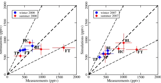
Averages are also computed for the clusters identified by K¨oppe et al. (2009) in the winter and summer troposphere in 2006 and 2007, independent on the location along the flight track between Frankfurt and Manila. A scatterplot of simu-lations and measurements is provided in Fig. 3. Agreement between observation and modelling is satisfactory for sum-mer and winter BL, for sumsum-mer HC, for FT in winter but not in summer, for TP in summer but not in winter. The model underestimates observations of the air mass maximum in FT during both 2006 and 2007 summers by around 50 % (1390 ± 310 pptv in 2007 and 1630 ± 330 pptv in 2006). The largest simulated value of 920±270 pptv is for 2007 summer BL, providing good agreement with the observation (the sec-ond largest observed annual value). Observed summer BL value is under estimated by only 30 % in 2006. The lowest observed values in winter and summer correspond to TP air masses that may have experienced some stratospheric influ-ence, which are then over-estimated by modelling. In HC air masses, comparison results depend on the year: the simula-tions underestimate measurements in 2006 but overestimate them in 2007. Observations show seasonal dependence for BL and FT air masses in 2006 and 2007, which is fairly well reproduced in 2007: averaged acetone vmr is smaller than 700 pptv in winter 2007 and is larger than 700 pptv in sum-mer 2007.
Given Fig. 3 and the frequency occurrence of air masses over the different zones, we may gain insight on the
8062 T. Elias et al.: Acetone variability in the upper troposphere
Figure 3. Relation between simulated and measured acetone vmr (pptv) for flights of 2006 and 2007 to Manila. Annual averages are derived from co-located simulations and airborne acquisition, making distinction according to the air mass fingerprint defined by Köppe et al. [2009], as FT for Free Troposphere, BL for Boundary Layer, HC for High Clouds and TP for tropopause. In winter 2007, dots not identified correspond to FT air mass. Vertical and horizontal bars depict the standard deviation of acetone simulated and measured, respectively. Superimposed are three lines showing agreement (x=y), and a factor 2 difference between simulation and measurement (y=2x and y=x/2).
Fig. 3. Relation between simulated and measured acetone vmr (pptv) for flights of 2006 and 2007 to Manila. Annual averages are derived
from co-located simulations and airborne acquisition, making distinction according to the air mass fingerprint defined by K¨oppe et al. (2009), as FT for Free Troposphere, BL for Boundary Layer, HC for High Clouds and TP for tropopause. In winter 2007, dots not identified correspond to FT air mass. Vertical and horizontal bars depict the standard deviation of acetone simulated and measured, respectively. Superimposed are three lines showing agreement (x = y), and a factor 2 difference between simulation and measurement (y = 2x and y = x/2).
comparison results per zone and season. In winter, satisfac-tory agreement is found only for BL in 2006 and for FT in 2007, for other air masses strong overestimations are found. Since they are both mostly encountered over CSChi, it is ex-pected to find best agreement in winter over CSChi, and an overestimation over other zones. Air mass origin maximum observed in summer FT air mass induces the geographical maximum observed over EurMed (Table 2). Moreover, ace-tone vmr being significantly under-estimated in FT air mass, it is expected to significantly underestimate acetone vmr over EurMed in summer. Satisfactory agreement for EurMed in 2006 and 2007 (Table 2) is therefore explained by an over-estimation in winter compensated by an underover-estimation in summer. Disagreement on the standard deviation confirms seasonal dependence is not reproduced (see Sect. 4.3). In contrary, as FT is being found in less than 10 % of the cases over CSChi in 2006 and 2007 summers, better agreement is expected over CSChi than over EurMed in summer.
4.2 Acetone variability over the Eurasian continent
We focus on flight segments embedded in the European and South Asian extended regions (last entries in Table 2) which both harbour net sources, and where nearly 25 % of the NH primary emissions and nearly 40 % of the NH chemi-cal production occurs, according to LMDz-INCA (Sect. 2). However on an annual basis, the regional atmospheric bur-den of acetone is proportional to the regional surface area (19 %) thanks to long-range transport on shorter time scales. As an example of modelled acetone transport in the UT, Fig. 2 shows that a plume observed over Central-South China
(CSChi) during the July 2007 also covers North India and the Himalayas. Moreover Europe and South Asia are the most intensively sampled regions by CARIBIC in 2006 and 2007. Indeed flights crossed EurMed 18 times, and Central-South China around 30 times (Table 2). The CARIBIC experi-ment thus allows studying the impact of acetone emission and transport on its spatial distribution in the UT over the Eurasian continent, as well as its seasonal variability.
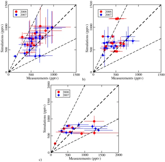
Scatterplots of 2006 and 2007 flight averages of co-located simulations and measurements are plotted in Fig. 4a, b and c for CSChi, SCSea and EurMed, respectively (Table 2). The flight average is the average of measured acetone vmr dur-ing the flight leg contained in the defined zone. Standard deviation on each flight represents the spatial variability in the zone. Modelling reproduces fairly well the variability of acetone vmr in the UT over CSChi (Fig. 4a) with only 30 % mean overestimation by LMDz-INCA, as well as over SC-Sea (Fig. 4b). Indeed averaged acetone vmr measured over CSChi varies by a factor of two in 2006 and by a factor of three in 2007, and simulated acetone varies by a factor of around 2.5 in 2006 and 2007. Measurement and simulation also agree concerning the standard deviation which can reach 400 pptv or 40 % of the flight average. The data points fall between the 100 %-agreement and the factor-2 overestima-tion lines, except for 6 outliers as the 2006 and 2007 min-ima. Agreement is particularly satisfactory for acetone vmr observed in excess of 800 pptv. Similarly, over SCSea, the flight average of acetone vmr varies by a factor of 2 to 4 in 2006 and 2007 according to observation over SCSea, and by a factor of around 2 according to modelling.
a) b)
c)
Figure 4. As Figure 3 except no distinction is made with air mass fingerprint but with geography and flight averages are plotted instead of seasonal averages: (a) Central-South China, (b) China Sea, and (c) Europe-Mediterranean region.
Fig. 4. As Fig. 3 except no distinction is made with air mass fingerprint but with geography and flight averages are plotted instead of seasonal
averages: (a) Central-South China, (b) China Sea, and (c) Europe-Mediterranean region.
Finally LMDz-INCA reproduces the magnitude of acetone vmr over EurMed but not its variability (Fig. 4c). The obser-vations indicate large variability of averaged acetone vmr as well as large standard deviations. Acetone vmr varies from less than 500 pptv to around 1400 pptv (except for the min-imum of 120 pptv measured in 2006 over North Africa, re-turning from Sao Paulo; Fig. 2). The summer maximum is consistent with retrievals from MIPAS-E (Moore et al., 2010) sounding the upper troposphere in August 2003: daily aver-ages vary between 1200 and 1600 pptv between 45◦N and 90◦N at 277 hPa. The standard deviation can reach values as high as 700 pptv for the 2006 maximum observed on 5 July 2006 due to a plume (Fig. 2). However modelling provides little variability, with averaged acetone vmr falling between 560±50 and 930±160 pptv in 2006 and 2007 (except for the minimum of 270 ± 10 pptv corresponding to the minimum observed over North Africa).
4.3 Annual cycle in the UT over Europe-Mediterranean, Central-South China and South China Sea
Sprung and Zahn (2010) discussed the annual cycle of ace-tone vmr in the stratosphere and at the tropopause over the Eurasian continent north of 33◦N, based on the 2006 and 2007 CARIBIC data. An annual cycle is observed, with minimum acetone vmr of 200 pptv in midwinter at the tropopause and maximum of 900 pptv in summer, but with large standard deviation reaching e.g. 60 % for the June maximum of 1000 pptv, due to stratospheric influence and geographical heterogeneity (latitude varying from 10◦E to
100◦E). We reduce such variability by focusing on the tropo-sphere and distinguishing measurements as a function of ge-ographical location. In 2006 and 2007, the CARIBIC aircraft route crossed the EurMed, CSChi and SCSea tropospheric regions almost every month (Table 2), providing the oppor-tunity to study the geographical variation of the annual cy-cle of acetone vmr in UT. The time series of flight averages
a) b)
c) d)
e) f)
Figure 5. Annual cycle of acetone vmr (pptv) simulated and measured in 7 months of 2006
and in 9 months of 2007 in UT over Central-South China (a and b) and the South China Sea (c
and d), and in 8 and 9 months of 2006 and 2007 respectively, over Europe-Mediterranean (e
and f). Black empty squares and red filled circles present simulated and measured averages,
respectively, with vertical bars for standard deviation. Intermittent line and shaded area
represent the climatological annual cycle: zonal average of monthly simulations, and its
standard deviation.
Fig. 5. Annual cycle of acetone vmr (pptv) simulated and measured in 7 months of 2006 and in 9 months of 2007 in UT over Central-South
China (a and b) and the South China Sea (c and d), and in 8 and 9 months of 2006 and 2007 respectively, over Europe-Mediterranean (e and f). Black empty squares and red filled circles present simulated and measured averages, respectively, with vertical bars for standard deviation. The intermittent line and shaded area represent the climatological annual cycle: zonal average of monthly simulations, and its standard deviation.
of co-located simulations and measurements plotted in Fig. 5 show that most of the variability observed for CSChi and SC-Sea (Fig. 4a and b) is due to the seasonal variation which is well reproduced by the model.
The annual CSChi maximum of 970 ± 400 pptv in 2006 is observed in October and in 2007 the maximum of 960 ± 300 pptv is observed in July (with largest standard deviation) (Fig. 5a–b). The 2006 and 2007 minima of 300 ± 60 and 150 ± 50 pptv, respectively, are observed in winter, when the variability is also at its minimum. The observed increase of
acetone vmr from winter to summer is reproduced by mod-elling, as averaged co-located simulations for 2007 show a minimum in winter and a maximum in July. In 2006, the minimum observed in December is overestimated, but the model reproduces the low value observed in spring.
Seasonal variation is as intense over the South China Sea (Fig. 5c–d) as over Central-South China in 2007, but in 2006 no clear tendency is observed over SCSea. The 2007 max-imum of 870 ± 150 pptv is observed in July (same day as over CSChi), and the minimum of 210 ± 50 pptv in March.
Agreement between model results and data is found in Au-gust 2007 over both SCSea and CSChi (flight back to Frank-furt, case study by Lai et al., 2010), however, strong over estimation occurs in autumn-winter 2006 and 2007 over SC-Sea. A plume is observed in October 2006 (Fig. 2), North West of the CSChi zone, extending to Central Asia, but it is simulated in the South East corner of the CSChi zone, also covering the entire SCSea zone. The plume location is not reproduced accurately but agreement is still found for aver-age and standard deviation over CSChi, while overestimation is significant over SCSea (Fig. 5c). Regarding inter-annual variability over SCSea, observations in June and July show important differences between 2006 and 2007, which how-ever are not captured by the model. In contrast, in April–May 2006 and 2007, modelling and observation agree to indicate that the acetone vmr is close to 500–600 pptv.
Finally, according to observation, acetone exhibits a strong annual cycle over EurMed (Fig. 5e–f). Flight averages as well as standard deviations increase significantly in June, July and August 2006 and 2007, reaching larger values than over SCSea and CSChi, and minimum is observed in Febru-ary 2006 and 2007, while, as discussed in the Sect. 4.2, modelling fails to simulate an annual cycle over EurMed. Agreement is satisfactory only for measured values around 750 pptv in spring.
4.4 Was the CARIBIC flight frequency sufficient to assess a climatological annual cycle of acetone?
Given the agreement between simulation and measurement in the UT over CSChi, modelling can be used to assess the effect of incomplete or sparse airborne sampling on the rep-resentativity of the annual cycle. The climatological annual cycle is plotted in Fig. 5 together with both the measured and simulated co-located annual cycle. The disagreement between the two approaches in representing the annual cy-cle shows the limitation of airborne sampling when acetone burdens are highly variable, as occurs in summer. The annual cycle sampled over CSChi agrees with the climatological cy-cle (Fig. 5a–b): the minimum of below 500 pptv, together with the minimum standard deviation, both occur in win-ter; and acetone vmr increases in both magnitude and stan-dard deviation towards summer. However, according to the monthly climatological average, the maximum should occur in September (2006 and 2007) with monthly averaged ace-tone vmr of around 1200 pptv, and neither in July, as ob-served in 2007, nor in October as obob-served in 2006. No measurements were made over CSChi in September 2006 and 2007 to check this simulated annual maximum. More-over measurements made in August 2007 suggest that ac-quisition frequency (once per month) in summer might not be sufficient to capture the maximum. Indeed observation and modelling agree, indicating that the acetone vmr at the time of aircraft crossing was smaller than the climatologi-cal monthly mean by more than 200 pptv (Fig. 5b). This is
an indication of significant day-to-day variability, which is moreover concomitant with strong spatial heterogeneity of the acetone in summer, shown by the increased standard de-viation. For winter, the climatological annual cycle provides confirmation that the acetone vmr is always over-estimated, but that simulated standard deviation is consistent.
Similarly over SCSea, the climatological annual cycle confirms overestimation in autumn-winter in UT, and that ob-servations are missing in September to check simulated max-imum around 1100 pptv. According to modelling, acetone distribution is more homogeneous in SCSea than in CSChi (except for May–June), as the climatological standard de-viation remains small, in contrast with observations. Sur-prisingly, the standard deviation of co-located simulations is large in March 2007 over SCSea, in contrast with measured standard deviation and with the climatological standard de-viation. This is because the aircraft unusually flew at a low altitude and that the simulated vertical gradient is too steep. This does not affect the climatological values which are de-fined at constant altitude of 238 hPa.
4.5 Acetone enhancement in the summer monsoon plume in the UT: horizontal heterogeneity and daily variability of acetone vmr
The summer acetone plume is responsible for the mean ace-tone vmr increasing from winter to summer, accompanied by increasing temporal and spatial heterogeneity. Simulations at 238 hPa for July 2007 (Fig. 2) show that the daily averaged acetone vmr is larger than 1000 pptv for a large zone covering North India, the Himalayas to the Chinese coasts, consistent with the extended South Asian region defined for the budget computation (Sect. 2). In accordance with the annual cy-cle over CSChi, the daily average of simulated acetone vmr over the extended South Asian region increases from 400 to 1000 pptv from winter to summer, with the standard devia-tion increasing from 100 to 400 pptv (Fig. 6). The standard deviation increases because the regional maximum increases from less than 1000 pptv in January–March to 3000 pptv in September, while the regional minimum remains relatively constant between 300 pptv in March and 500 pptv in Novem-ber. The area covered by the acetone plume also increases from winter to summer, to cover half the South Asian region. Figure 6 also shows that day-to-day variability can be very important, as the sudden decrease of more than 1000 pptv around September–October.
Observations show that the acetone variability within a single day can be large. Over CSChi, the time lag between inbound and outbound flights is generally between 10 and 17 h, while over SCSea it is less than 8 h. This in-out shift can mean 240 pptv difference, as for August 2006 over SC-Sea and for August 2007 over CSChi (Fig. 5). Shifts can be large even when modelling indicates a homogeneous acetone field. Examples are the 200 pptv change in February 2007 over CSChi and in October 2007 over SCSea. The in-out
Fig. 6. Temporal and horizontal variability of acetone vmr (pptv) at
238 hPa over South Asia. Daily averages are provided by LMDz-INCA. The dashed line represents the regional average, with the shaded zone for ±1 standard deviation. Full lines show spatial min-imum and maxmin-imum acetone vmr for each day. Monthly number of values larger than 1000 pptv is indicated at the top of the figure.
shift may be due to altitude differences, as the outbound flights over SCSea are generally higher by 20 hPa than the inbound flights, but lower than inbound flights over CSChi by more than 70 hPa. However the change of acetone vmr with altitude is not systematic. The acetone vmr is sometimes observed to decrease with increasing altitude, as in August and November 2006 over SCSea, and sometimes observed to increase with increasing altitude as in May 2007. Over CSChi, the acetone vmr decreases with increasing altitude in April and November 2006, and in February, June and August 2007, but remains constant despite altitude change in May and October 2007. Other causes may be the different insola-tion condiinsola-tions and the air mass change with time.
4.6 Effects of vertical gradients
Acetone vmr may depend on flight altitude as modelling shows. Simulated monthly vertical profiles are plotted in Fig. 7, for 2 cases: (1) background conditions defined by ace-tone vmr at 238 hPa being below 1000 pptv, (2) “ppbv-event” conditions defined by acetone vmr at 238 hPa larger than 1000 pptv. During background conditions, the acetone vmr continuously monotonically decreases with altitude. In con-trast, during the ppbv-event, a local minimum is simulated between 400 and 600 hPa, indicating an elevated acetone plume (except for September, when the plume seems to ex-tend down to the surface with acetone vmr remaining higher than 1300 pptv below 238 hPa). The largest values at surface level are reached during the 238-hPa ppbv-events: from May to November, the acetone vmr is larger than 2500 pptv, and even reaches 3400 pptv in July, while under background con-ditions acetone vmr is less than 2200 pptv. The simulated
al-Fig. 7. Vertical profile of monthly average of acetone vmr simulated
by LMDz-INCA over South Asia extended region, in background conditions and during 238-hPa ppbv-event (238-hPa acetone vmr >1000 pptv).
titude of the acetone plume is consistent with simulations by Park et al. (2004) of a plume composed of high mixing ratios of CH4, H2O and NOxat pressure altitudes included between 300 and 150 hPa, in accordance with observations from the HALOE instrument. The increase of CH4 is also observed by the AIRS instrument in the altitude interval from 300 to 150 hPa (Xiong et al., 2009).
While modelling over EurMed does not reproduce the ob-served variability of acetone in the UT, it does provide vari-ability at surface level. Simulated vertical profiles over Eu-rope (not shown) are similar to vertical profiles over South Asia under background conditions only (no ppbv-events were observed at 238 hPa). While the averaged acetone vmr remains constant around 600 pptv at 238 hPa, it varies be-tween 1300 and 2200 pptv at surface level, in correlation with the season. Comparisons are made with ground-based obser-vation presented by Solberg et al. (1996) and already used by e.g. Jacob et al. (2002) and Folberth et al. (2006). Time series of monthly averages of acetone vmr are plotted for 6 European sites in Fig. 8. Similarly to the observations in the UT, an annual cycle is observed at the surface sites, but it is highly dependent on location. The timing and magnitude of the maxima varies: the maximum is observed from May in Birkenes to August in Donon, between 1000 pptv in Rucova and 2000 pptv in Donon. The minimum is observed between 300 pptv in Birkenes and 600 pptv in Waldhof. In contrast to the UT, the model is able to simulate an intense annual cycle at surface level, with acetone vmr increasing by a fac-tor 2.5 from winter to summer. The maximum is simulated in August-September, somewhat later than observed, except in June in Birkenes, in agreement with observation. Agree-ment between modelling and observation is satisfactory in spring-summer at the two 48–49◦N sites. The maximum
Fig. 8. Annual cycle of acetone vmr measured at surface level at 6 European stations (Solberg et al., 1996) (dots for averages and vertical
bars for standard deviation), and climatological annual cycle computed by LMDz-INCA (line).
magnitude is reproduced, but the minimum is overestimated, as it is the case in the UT over Central-South China and South China Sea. The acetone vmr is over estimated in autumn and winter, except in Waldhof in January–March. For the 56– 58◦N sites of Birkenes and Rucova, modelling constantly overestimates the observations by 500 to 1000 pptv.
Systematic overestimation in autumn (for all sites) is sim-ilar to Jacob et al. (2002) a priori modelling, which was at-tributed to an overestimated emission from plant decay as an acetone source peaking in September–October. Jacob et al. (2002) then proposed reducing the global plant decay
contribution to fit measured annual cycles. A shift to au-tumn in the annual cycle has also been simulated with the LMDz-INCA model (in the 60–90◦N latitude) for methanol which is another oxygenated species (Dufour et al., 2007). The authors attribute the accumulation of methanol to long residence time. Thus increasing land deposition in autumn and winter might improve agreement with observation for methanol, and it could also be envisaged for acetone.
a)
b)
c)
d)
e)
Figure 9. KNMI/ECMWF 5-day air mass back-trajectories. Coordinates and dates of arrival
points correspond to plumes sampled along the 2006 and 2007 July flights (Figure 2).
Fig. 9. KNMI/ECMWF 5-day air mass back-trajectories. Coordinates and dates of arrival points correspond to plumes sampled along the
2006 and 2007 July flights (Fig. 2).
4.7 Two contrasted transport conditions: rapid uplifting of pollutants over Central-South China and long-range transport to Europe-Mediterranean region
We have described how acetone vmrs are under-estimated in summer FT air masses encountered over Europe-Mediterranean region, and how better agreement is found in summer BL and HC air masses sampled over Central-South China. We discuss here the impact of different transport con-ditions, which implies different chemical activity in the
trans-ported air masses, witnessed by a different relation between acetone content and CO and O3contents.
Five-day back-trajectories are computed based on meteo-rological analysis data from the European Centre for Medium range Weather Forecasts (ECMWF) (van Velthoven, 2009), with the KNMI trajectory model TRAJKS (Scheele et al., 1996) for every 3 min of flight. Back-trajectories plotted in Fig. 9 are computed for plumes observed in July 2006 and 2007. Two plumes are observed, with acetone vmr in excess of 2000 pptv around 21:40 GMT 5 July 2006, and in excess of 1000 pptv around 05:20 GMT 6 July 2006. Three plumes
T. Elias et al.: Acetone variability in the upper troposphere 8069
a)
b)
c)
d)
e)
Figure 9. KNMI/ECMWF 5-day air mass back-trajectories. Coordinates and dates of arrival
points correspond to plumes sampled along the 2006 and 2007 July flights (Figure 2).
Fig. 9. Continued.
are observed with acetone vmr in excess of 1500 pptv around 22:10 GMT 17 July 2007, in excess of 1000 pptv around 04:10 GMT 18 July 2007, and in excess of 1500 pptv around 06:20 GMT (Fig. 2). The European plume, assigned to the FT air mass cluster in July 2007 (no air mass assigned in July 2006), originates from long-range transport from North America or the North Atlantic Ocean. The North Chinese plume, with mainly HC and few BL signatures, originates from the local boundary layer with only few days of travel time (Fig. 9d), and the South Chinese plume, with BL signa-ture, originates from regional transport from India (Fig. 9e).
The transport conditions over China are similar to the im-pact of the summer monsoon observed over India, which was the subject of many publications. The summer mon-soon affects the composition of the UT by dynamical and meteorological processes, basically strong and rapid con-vection lifting of boundary layer air masses combined with high precipitation affecting emissions from certain sources. Consistent enhancements of CO, H2O, CH4, N2O and non-methane hydrocarbons were observed with CARIBIC over South Asia in summer 2008 (Schuck et al., 2010; Baker et al.,
2011). A concomitant decrease of ozone was also observed by CARIBIC (Schuck et al., 2010). Model and satellite data consistently localised high mixing ratios of CH4 between 60◦E and 120◦E around 30◦N, a region included in our
ex-tended South Asian region (Table 2) at and above cruising altitude, at pressure altitudes between 300 and 100 hPa (Park et al., 2004; Xiong et al., 2009). Schuck et al. (2010) showed that air masses sampled north of 30◦N generally travel for more than a week, in contrast with air masses south of 30◦N which had ground contact within the last four days prior to sampling. Baker et al. (2011) confirmed that in the southern monsoon region, sampled air masses travelled 3 to 6 days before sampling, and 9 to 12 days in northern monsoon re-gion. This is consistent with the summer BL air mass fin-gerprint mostly encountered over CSChi and SCSea (in 2006 and 2007), but rarely encountered over Northern Asia.
The CARIBIC data set shows that air masses sampled over EurMed and CSChi bear different chemical signatures. The chemical signature is deduced from the CARIBIC measure-ments of O3and CO vmrs. Values of CO vmr larger than 140 ppbv occur only over CSChi and SCSea in 2006, and
8070 T. Elias et al.: Acetone variability in the upper troposphere
Figure 10. Acetone/CO signature in various air masses sampled in 2006 and 2007 summers. Linear regressions are plotted in red for HC and BL air masses sampled over CSChi, in purple for these same air masses but sampled over EurMed and Central Asia (CAs) and in black for all FT air masses sampled everywhere.
Figure 11. O3/CO signature of same air masses of Figure 10, but as O3 vmr plotted as a function of CO vmr.
Fig. 10. Acetone/CO signature in various air masses sampled in
2006 and 2007 summers. Linear regressions are plotted in red for HC and BL air masses sampled over CSChi, in purple for these same same air masses but sampled over EurMed and Central Asia (CAs) and in black for all FT air masses sampled everywhere.
not over other regions. A maximum of CO vmr of 260 ppbv is measured over CSChi in July and August 2006 (for ace-tone vmr around 1700 pptv). However, over EurMed, CO vmr is never observed larger than 120 ppbv. CO vmrs in-creasing with acetone vmrs, the slope of acetone versus CO identifies the sampled air mass (de Reus et al., 2003). Lin-ear regressions with high correlation coefficient are plotted in Fig. 10, for HC, FT, and BL air masses sampled in 2006 and 2007 summers. The slope depends on the air mass type but might also depend on location. In particular for BL and HC air masses, the slope is steeper over EurMed and Central Asia (around 25 pptv acetone ppbv−1CO) than over CSChi (around 6 pptv acetone ppbv−1CO). The FT slope (rejecting outliers with CO vmrs larger than 120 ppbv) seems closer to the BL and HC slopes over EurMed and Central Asia (around 16 pptv acetone ppbv−1CO).
Over East Mediterranean, major contrast was found by Scheeren et al. (2003) in the chemical composition of the upper troposphere, between air mass origin over North At-lantic/North America (farther west than 0◦) and over South Asia (farther east than 40◦E). O3vmrs were smaller in South Asian air masses than in North Atlantic/North America air masses (while CO vmr was larger). Similar behaviour is ob-served here in relation to the classification per both region and air mass fingerprint (Fig. 11). Enhancement of both gases never occurs simultaneously, CO vmrs increase only in HC and BL air masses sampled over CSChi, with O3 re-maining smaller than 100 ppbv. O3vmr can increase in FT air masses and in HC and BL air masses over EurMed up to 150 ppbv, but with CO vmr remaining smaller than 130 ppbv.
Figure 10. Acetone/CO signature in various air masses sampled in 2006 and 2007 summers. Linear regressions are plotted in red for HC and BL air masses sampled over CSChi, in purple for these same air masses but sampled over EurMed and Central Asia (CAs) and in black for all FT air masses sampled everywhere.
Figure 11. O3/CO signature of same air masses of Figure 10, but as O3 vmr plotted as a function of CO vmr. Fig. 11. O3/CO signature of same air masses of Fig. 10, but as O3
vmr plotted as a function of CO vmr.
5 Conclusions
The purpose of this work is to: (1) describe spatial distri-bution and temporal variability of acetone vmr in the UT; (2) propose benchmarks deduced from the observation data set; and (3) investigate the representativeness of the obser-vational data set. The approach consists in comparing two data sets obtained by observation and modelling. Simula-tion results are provided by LMDz-INCA, a global chem-istry climate model including the oxidation of methane and volatile organic compounds. The CARIBIC experiment pro-vides acetone measurements in the upper troposphere (UT) mainly over north hemisphere continental regions where ma-jor sources are located and where chemical activity signifi-cantly contributes to acetone sources and sinks. Acetone is a key factor in UT chemistry, as a potential source of hydroxyl and hydroperoxyl radicals, which are important components of the ozone cycle.
Measurements were made aboard intercontinental flights to explore the influence of different air mass history, long-range transport in the free troposphere, rapid convective uplifting of boundary layer compounds, as well as con-tinent/ocean contrasts. Moreover the regularity of the CARIBIC measurements (monthly flights) over several years provides insight on seasonal variability of the acetone con-tent. Consecutive inbound and outbound flights separated by a short stopover on almost identical routes also allow defin-ing the sensitivity of the chosen flight track in relation to the specific plume transport. Strong variability is observed. Al-most a factor 2 on acetone vmr is related to geography, in par-ticular an East-West gradient is observed over the Eurasian continent, with annual average of around 450±200 pptv over South China Sea and of around 800 ± 500 pptv over Europe-Mediterranean region. Ocean/continent contrast is also ob-served with a 50 % enhancement over the continent. On a