HAL Id: halshs-00849072
https://halshs.archives-ouvertes.fr/halshs-00849072
Preprint submitted on 30 Jul 2013
HAL is a multi-disciplinary open access
archive for the deposit and dissemination of
sci-entific research documents, whether they are
pub-lished or not. The documents may come from
teaching and research institutions in France or
abroad, or from public or private research centers.
L’archive ouverte pluridisciplinaire HAL, est
destinée au dépôt et à la diffusion de documents
scientifiques de niveau recherche, publiés ou non,
émanant des établissements d’enseignement et de
recherche français ou étrangers, des laboratoires
publics ou privés.
Estimating Gender Differences in Access to Jobs
Laurent Gobillon, Dominique Meurs, Sébastien Roux
To cite this version:
Laurent Gobillon, Dominique Meurs, Sébastien Roux. Estimating Gender Differences in Access to
Jobs. 2013. �halshs-00849072�
WORKING PAPER N° 2013 – 25
Estimating Gender Differences in Access to Jobs
Laurent Gobillon
Dominique Meurs
Sébastien Roux
JEL Codes: J16, J31, J71
Keywords: Gender, Discrimination, Wages, Quantiles, Job assignment model,
Glass ceiling
P
ARIS
-
JOURDAN
S
CIENCES
E
CONOMIQUES
48, BD JOURDAN – E.N.S. – 75014 PARIS TÉL. : 33(0) 1 43 13 63 00 – FAX : 33 (0) 1 43 13 63 10
Estimating Gender Di¤erences in Access to Jobs
Laurent Gobillon
yDominique Meurs
zSébastien Roux
xJuly 5, 2013
Abstract
This paper proposes a new measure of gender di¤erences in access to jobs based on a job assignment model. This measure is the probability ratio of getting a job for females and males at each rank of the wage ladder. We derive a non-parametric estimator of this access measure and estimate it for French full-time executives aged 40 45in the private sector. Our results show that the gender di¤erence in the probability of getting a job increases along the wage ladder from 9% to 50%. Females thus have a signi…cantly lower access to high-paid jobs than to low-paid jobs.
Keywords: gender, discrimination, wages, quantiles, job assignment model, glass ceiling. JEL Classi…cation: J16, J31, J71
We thank Joseph Altonji, Christian Bontemps, Allison Booth, Moshe Buchinski, Pierre Dubois, Francis Kramarz, Thierry Magnac, Ronald Oaxaca, Patrick Puhani, Jean-Marc Robin, Bernard Salanié and two anonymous referees for their useful comments, as well as the participants of seminars and conferences at the University of Hanover, INED (Paris), CREST (Paris), University of Toulouse, Paris School of Economics, University of Paris Ouest Nanterre, World Congress of the Econometric Society (Shangai), ESEM (Barcelona), EALE (Tallin). All remaining errors are ours.
yINED, PSE, CEPR and IZA. Address: Institut National d’Etudes Démographiques (INED), 133 Boulevard Davout, 75980 Paris
Cedex 20, France. Email: [email protected].
zUniversity of Paris Ouest Nanterre (EconomiX) and INED. Address: Institut National d’Etudes Démographiques (INED), 133
Boulevard Davout, 75980 Paris Cedex 20, France. Email: [email protected].
xDARES and CREST. Centre de Recherche en Economie et Statistique (CREST), 15 Boulevard Gabriel Péri, 92245 Malako¤ Cedex,
1
Introduction
Females are under-represented in high-paid occupations and this fact explains a large part of the gender wage di¤erential. In this paper, we propose a formal way to quantify the gender di¤erence in access to each position along the job ladder and to assess whether females have a lower access to high-paid jobs than to low-paid jobs.
Since Albrecht, Bjorklund and Vroman (2003), quantile regressions have been used to estimate the di¤erence between the conditional wage distributions of males and females. It is said to be a “glass ceiling e¤ect” when this gap gets wider in the upper tail. This widely used approach is fruitful to highlight the gender bias in promotions but it remains purely descriptive.
We propose a more precise measure of this gender bias which can be justi…ed with a microfounded framework. Our work builds on the literature on job assignment models which posits the existence of heterogenous job positions (see Sattinger, 1993; Teulings, 1995; Fortin and Lemieux, 2002; Costrell and Loury, 2004). In our framework, each position is characterized by a speci…c wage o¤er to applicants. Some male and female workers apply for the best-paid job. Males and females are characterized by di¤erent chances of getting this speci…c job. The manager of the best-paid job selects a worker among applicants accordingly. The manager of the second best-paid job hires an individual among the remaining workers, and so on. We de…ne an access function as the probability ratio of females and males getting a job of a given rank. This access function captures not only labor demand e¤ects, such as gender discrimination in the hiring process for some job positions, but also labour supply e¤ects, such as gender di¤erences in preferences for job positions depending on time constraints.
In an empirical section, we estimate this access function on full-time executives aged 40 45 working in French private and public …rms. We …nd that at the bottom of the wage distribution (5thpercentile), the probability of
females getting a job is 9% lower than that of males. The di¤erence in probability is far larger at the top of the wage distribution (95thpercentile) and climbs to 50%. Females thus have a signi…cantly lower access to high-paid jobs than to low-paid jobs.
Our analysis is related to a few empirical studies which investigate the gender di¤erence in promotions. Blackaby, Booth and Frank (2005) …nd a signi…cant gender promotion gap on the UK academic labour market after controlling for productivity di¤erences. Pekkarinen and Vartiainen (2006) show on Finnish data that among blue-collar workers, females have to reach a higher productivity threshold to get promoted than males. This kind of research is limited to case studies as it exploits detailed information on the individual ranking along the job ladder in a speci…c sector. Here, we consider the whole private sector and postulate that the wage is a reasonable proxy for the position in the job hierarchy: a higher wage corresponds to a better position. The wage has already been used by Bertrand
and Hallock (2001) to de…ne the group of top corporate jobs which is shown to include only 2:5% of women.1 In
fact, results obtained by Baker, Gibbs and Holmstrom (1994) on a single …rm support the fact that the rank of a position in the job hierarchy is correlated with the wage, although the wage is not strictly attached to the job. Killinsworth and Reimers (1983) argue that neither the type nor the rank of a position is perfectly indexed by the wage. This is particularly true for blue collars, for whom wages increase signi…cantly with job tenure. Also, some blue collars occupy jobs which are paid at the minimum wage but do not correspond to the same hierarchical position. Hence, we restrict our attention to executives whose wage re‡ects more closely the rank along the job ladder. We only analyse full-time workers aged 40 45 who should constitute a rather homogenous population. Additionally, the e¤ect of supply side factors for female full-time executives aged 40 45 should be rather limited.2
Our results show that females have a lower access to jobs than males at all ranks in the wage distribution. Moreover, their access to jobs decreases along the job ladder. We also conduct our analysis for speci…c industries as they constitute more homogenous labour markets. We consider more speci…cally banking and insurance as they are labour intensive with a large share of females and have contrasting wage policies in France. Banks rely on a rigid job classi…cation inherited from the early eighties when they belonged to the public sector. By contrast, insurance companies propose much more individualized careers. Females are found to have a far better access to high-paid jobs than males in the banking industry than in the insurance industry. Results on pooled industries, insurance and banking are qualitatively in line with the usual interpretation of the gender quantile wage di¤erence increasing with the rank.
We then stratify our estimation of the access function by group de…ned from age, labour market experience or country of birth (France or foreign country). Results are very similar across groups. This is in line with our use of an homogeneous population. We also make an alternative assumption on the size of the labour market, assuming that the competition of workers for jobs occurs within each …rm rather than on the national market. We estimate the average access function across large …rms employing more than 150 full-time executives aged 40 45. When pooling all industries, results are quite similar to those obtained when competition is supposed to occur on the national market. For the speci…c insurance industry, results are a bit di¤erent, as we …nd that the gender di¤erence in access to high-paid jobs is slightly less pronounced. This change is generated by some heterogeneity in the level of wages among …rms. Finally, we show that our results on the lower access of females to high-paid jobs are robust when workers occupying lower ranking jobs than executive positions are included in the sample.
In the last section, the access function is micro-founded with three theoretical mechanisms that can lead to a
1Note that when there is occupational segregation, people can have the same responsibilities but di¤erent position titles. Females
can be lower in the job hierarchy and get lower wages than males while doing the same job. This occurs for instance when a female has an administrative title but does part of the job of a male having a vice-president title.
2It can still be argued that, for a given job position, females bargain less for the wage than males and may end up earning less at the
same hierarchical level (Babcock and Lashever, 2003). However, in France, wage levels are strongly related to job titles, and females are usually paid less than males only when they occupy a lower position in the job hierarchy.
lower access of females to high-paid jobs. The …rst one is based on gender di¤erences in labour supply. We consider that males and females have ex-ante the same distribution of productivity but are heterogenous in their labour supply. We show that the access function is decreasing if the di¤erence in job application rates between females and males increases along the job ladder. The second mechanism is based on taste discrimination (Becker, 1971). It is straighforward to show that the access function is decreasing if the preference for females relative to males decreases along the job ladder. Finally, the third mechanism is a version of statistical discrimination where the distribution of skills is the same for males and females but skills are observed with more noise for females than for males (Aigner and Cain, 1977; Coate and Loury, 1993; Cornell and Welch, 1996).3 We show that statistical
discrimination can then lead to a decreasing access function. This can occur because skilled males are more often hired for high-paid jobs as their skills are observed with less uncertainty. Males looking for less-paid jobs are those not selected for high-paid positions and they are on average less skilled than females. As a consequence, the hiring rate of males for less-paid jobs is lower than for high-paid jobs. The three mechanisms can occur simultanously and the empirical access function captures the aggregate of the three explanations.
The rest of the paper is organized as follows. In section 2, we present our framework. Our econometric strategy to estimate the access function is detailed in section 3. We then describe our dataset and report some stylized facts in section 4. We comment our estimation results in section 5. We conduct some robustness checks when taking into account the individual observed heterogeneity and segmented markets in section 6. Some additional robustness checks such as the inclusion in the sample of workers unable to access an executive position are proposed in section 7. In section 8, we present three theoretical mechanisms that can generate a decreasing access function. Concluding remarks are given in the last section.
2
The framework
2.1
Our model
We propose a job assignment framework that allows to consistently measure the gender di¤erences in access to jobs. Consider a countable number of workers applying for a countable number of job positions. There is a proportion nm of males in the whole population of workers, which we refer to as the measure of males for clarity hereafter,
and a measure nf = 1 nmof females. For simplicity, we assume that there is a bijection between workers and job
positions. This assumption rules out the existence of workers not being hired and job positions not being …lled. It will be relaxed in Section 7.
A worker is primarily interested in the job yielding the highest wage. Job positions are heterogenous such that
3Another version of statistical discrimination posits a gender di¤erence in average productivity (Arrow, 1971; Phelps, 1972) but we
think it is more interesting to show that a decreasing access function can be obtained without di¤erences in the intrinsic characteristics of the male and female subpopulations.
each job position is associated with a speci…c …xed wage through a contract. This wage is not allowed to depend on the gender of the applicant. We suppose that two job positions cannot be associated with the same wage o¤er so that each job can be uniquely identi…ed by its rank in the wage distribution.4 Workers …rst consider the best
ranked position as it o¤ers the highest wage. Those who are not hired turn to the second best ranked position, and so on.
For any job position of given rank u, there is a measure denoted nj(u) of gender-j workers considering the job
(ie. all the gender-j workers not hired for jobs of higher rank). We have nj(1) = nj as all workers consider the
…rst job and nj(0) = 0 as all workers end up being employed.
We can then determine for each gender j a di¤erential equation which is veri…ed by the measure of available workers at each rank. Consider an arbitrarily small interval du in the unit interval. The proportion of jobs in this small interval is du since ranks are equally spaced (and dense) in the unit interval. The instantaneous probability of a gender-j worker getting a job in this interval is denoted j(u). This probability can vary with gender for various reasons such as di¤erences in labour supply (a di¤erent share of males and females considering that work conditions are too constraining to apply), taste discrimination against females or statistical discrimination against females. We discuss in Section 8 how the instantaneous probability can be micro-founded theoretically to embed these three explanations.
It is possible to relate the instantaneous probabilities of getting a job with the process through which jobs are …lled. The measure of jobs occupied by workers of a given gender j is nj(u) j(u) du. For this gender, the measure
of workers available for a job of rank u du can be deduced from the measure of workers available for a job of rank u substracting the workers who get the jobs of ranks between u du and u :
nj(u du) = nj(u) nj(u) j(u) du (1)
From this equation, we obtain when du ! 0:
n0j(u) = j(u) nj(u) (2)
This relationship states that the instantaneous variation in the measure of gender-j workers around rank u depends on the stock of gender-j workers and their chances of getting a job.
We now introduce a measure of relative access to jobs. Consider one male worker and one female worker available for a job position of given rank u. These two workers have di¤erent probabilities of being hired as they are not of the same gender. We can characterize the gender di¤erence in access to jobs with the function de…ned as the probability ratio of a female and a male being hired for the job position:
h (u) f(u)
m(u)
(3)
4The wage distribution is supposed to be exogenous. We could introduce some mechanisms on the labour market to endogenize this
This function h ( ) measures the gender relative access to jobs and we label it the “access function”. It should be kept in mind that this function captures not only labour demand e¤ects impeding the access of females to some job positions, but also labor supply e¤ects related to gender di¤erences in preferences. When the access function takes the value one at all ranks, males and females have the same chances of getting each job position. When the access function takes a value lower than one for a job position of given rank, females have less chances than males of getting the job.
It is then possible to formally de…ne a lower access to high-paid jobs than to low-paid jobs for females: De…nition 1 Females have a lower access to high-paid jobs than to low-paid jobs if there are some ranks u0
and u1 such that for any u 2 ]u0; u1[ and v > u1, we have h (u) > h (v) and h (v) < 1.
For instance, females have a lower access to high-paid jobs than to low-paid jobs when the access function is continuous, strictly decreasing and takes some values lower than one at the highest ranks. It is also the case when the access function is a two-step function with the second step at a value lower than the …rst step and lower than one. In particular, an interpretation of the speci…cation where the second step takes a zero value is the existence of a glass ceiling.5 In practice, a lower access to high-paid jobs can be contrasted to a uniform access to all jobs
when the access function is constant at all ranks.
2.2
Gender quantile di¤erences
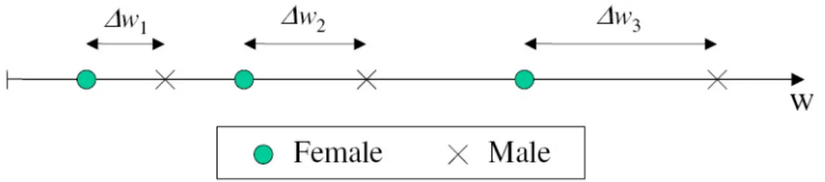
The recent empirical literature on the glass ceiling has focused on the di¤erence between the quantiles of the wage distributions of males and females. Typically, when this di¤erence increases with the rank, it is usually said that there is a glass ceiling. We believe that this approach confuses two dimensions, the job position and the associated wage, possibly leading to inaccurate interpretations. Figure 1 presents a simple scheme illustrating this point. Suppose a classic job ladder where the wage increases more than proportionally with the rank in the wage distribution. Positions are occupied alternately by a female and a male. The gender quantile di¤erence for high-paid jobs is larger than for low-paid jobs, which means that the gender wage gap widens along the job ladder. It is tempting to conclude that there is a glass ceiling e¤ect (according to the loose labelling of the literature), but this interpretation is questionable as the odds of a female (or a male) occupying a position are roughly constant along the job ladder.
[Insert F igure 1]
In fact, this intepretation does not rest on any straightforward rationale and has two caveats. First, it does not control for the spacing between wages and thus mixes the ranks of positions on the job ladder with earnings. Second,
5Very often in the literature, the glass ceiling is more loosely de…ned. It is considered that there is a glass ceiling e¤ect when females’
the rank at which quantiles are computed has a di¤erent meaning for the two genders. For males, it corresponds to the rank in the wage distribution of males. For females, it corresponds to the rank in the wage distribution of females.
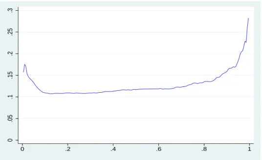
We now show that it is possible to generate from our framework a gender quantile di¤erence which increases with the rank even if there is no glass ceiling and the di¤erence in access to jobs between males and females is the same at all ranks. We …rst solve the model when the access function is constant with h (u) = :672 at all ranks and the proportion of females is that of the banking industry (28:7%).6 The numerical solution allows to compute
vj(u) = njn(u)j as well as uj= vj1which gives for a job of given rank in the wage distribution of gender j, its rank
in the wage distribution of job positions.7 We can then relate the quantile function of gender j denoted
j( ) to the
quantile function of job positions ( ) through the relationship: j(v) = [uj(v)]. The gender quantile di¤erence
is given by:
( m f) (v) = [um(v)] [uf(v)] (4)
We can compute the gender quantile di¤erence using the solution uj( ) of the model and the wage distribution
of job positions in the banking industry for ( ). The gender quantile di¤erence represented on Figure 2 is an increasing function above rank :6. Whereas the increase is small just above that rank, the curve becomes very steep above rank :9. The literature would conclude to a glass ceiling whereas there is none.
[ Insert F igure 2 ]
Hence, economic interpretations should rather rely on the primitive function of a model which is the access function in our case. We now propose an econometric approach to estimate the access function non parametrically from the data.
3
Estimation strategy
We now show how the access function can be estimated non-parametrically from a cross-section dataset containing for each worker some information on gender and wage. First recall that the access function can be reinterpreted as
6These choices are made clear in the empirical section. Indeed, we will show that the gender di¤erence in access to jobs is nearly
uniform in the banking industry and that the access function takes values close to :672 at all ranks.
7We determine numerically for each gender the measure of available workers at each rank at the equilibrium. For females, we use the
algorithm proposed by Bulirsch and Stoer (for the implementation, see Press et al., 1992, p. 724-732) to solve the di¤erential equation giving nf( ). As all jobs are …lled, we have: nf(u) + nm(u) = u. Deriving this equality, we get: n0m(u) = 1 n0f(u). Using (2) for the
two genders, we get: n0
f(u) =n0m(u) = h (u) nf(u) =nm(u), which is equivalent to n0f(u) =
h 1 n0
f(u)
i
= h (u) nf(u) = u nf(u).
Rewriting this expression to get an expression of n0f(u), we obtain: n0f(u) = u nnf(u)h(u)
f(u)+nf(u)h(u). This di¤erential equation is solved
backward from the highest to the lowest rank using the initial condition nf(1) = nf. After the di¤erential equation for females has
been solved, we deduce the solution for males using the relationship nm(u) = u nf(u). It is then straightforward to compute vj( )
the unit probability ratio of females and males getting a given job. From equation (2), each unit probability can be rewritten as: j(u) = n0 j(u) nj(u) (5) We introduce for gender-j workers, the random variable corresponding to their rank in the wage distribution of job positions, Uj. The cumulative (resp. density) of this variable is denoted FUj (resp. fUj). The cumulative veri…es the relationship: FUj(u) = nj(u) =nj. Hence, each unit probability can be rewritten as:
j(u) =
fUj(u) FUj(u)
(6) The numerator and denominator of the gender-j unit probability only depend on the distribution of ranks of gender-j workers in the wage distribution of job positions. This means that in practice, the ranks of workers of each gender in the distribution of job positions are su¢ cient to estimate the unit probabilities, and thus the access function. These ranks can be computed very easily from the data.
For each gender, the numerator and denominator of the unit probability of getting a job can be evaluated using the usual Rosenblatt-Parzen Kernel estimator of the density fUj( ) which is given by:
e fUj(u) = 1 !jNj X ijj(i)=j K u ui !j (7)
where K ( ) is a Kernel, !j is the bandwidth, j (i) is the gender of individual i and ui is his/her rank in the wage
distribution of job positions. A standard estimator of the cumulative FUj( ) is then given by: e FUj(u) = u Z 0 e fUj(u) du = 1 Nj X ijj(i)=j L u ui !j (8) where L (u) = u Z 1
K (v) dv. However, we expect the estimators efUj( ) and eFUj( ) to perform quite poorly for ranks close to zero and one as standard non-parametric estimators are asymptotically biased at the boundaries (see Härdle, 1990).
Therefore, we rather consider some estimators based on local polynomial approximations in line with Jones (1993) and Lejeune and Sarda (1992). The density and cumulative functions evaluated at a given rank u are obtained by minimizing: min ; Z 1 0 K u v !j [gj(v) (u v)]2dv (9)
where gj is either the empirical density function de…ned as gj(v) = Nj 1
P
ijj(i)=j ui(v) where u(v) is the Dirac delta function associated to v, or the empirical cumulative function de…ned as gj(v) = Nj 1
P
ijj(i)=j1fui vg. The estimators of the density and cumulative functions at rank u, denoted bfUj(u) and bFUj(u), are given by the value of derived from their respective minimization program. Here, the boundary problem is taken into account by
simply …xing the bounds of the integral in (9) to zero and one.8 The bias at these boundaries is of order O !2 j
and tends to zero when the bandwidth tends to zero.
In our application, the Kernel is chosen to be Epanechnikov and we experiment with values of bandwidth which are multiples of the value given by the rule of thumb (Silverman, 1986).9 Whereas the overall shape of the access
function does not change for multiples between :5 and 4, there are some slight variations at ranks below :03. To avoid undersmoothing at small ranks because density and cumulative functions are estimated with fewer workers, we decided to use a bandwidth which is equal to two times the value given by the rule of thumb. Note that the Epanechnikov kernel takes the value zero outside the interval [ !j; !j]. It is possible to show that because of this
property, the estimator of the density obtained from (9) takes exactly the same value as the estimator given by (7) for ranks in the interval [!j; 1 !j]. In fact, the two estimators for the density computed at points in this
interval coincide because there is no boundary problem.10 Technical details to obtain some analytical formulas for
the estimators are given in Appendix A.
For gender j, an estimator of the unit probability of getting a job can then be computed as bj(u) = bfUj(u) = bFUj(u). We …nally obtain an estimator of the access function:
bh (u) = bf(u)
bm(u) (10)
This estimator is computed for a grid of 1000 ranks in [0; 1] which are equally spaced. The con…dence interval of the access function at each rank is computed by bootstrap with replacement (100 replications).11
It is also possible to adopt a parametric speci…cation of the access function and estimate the parameters from a minimization program as shown in Appendix B. More speci…cally, we consider the linear speci…cation h (u) = a b:u where a is the access to jobs at the lowest rank and b captures a decrease or an increase in access to jobs with the rank. A test of the linear speci…cation using the Cramer Van-Mises statistic is also provided.
8If, instead, the bounds of the integral in (9) were …xed to 1 and +1, the estimators of the density and cumulative would turn
out to be the usual kernel estimators given by (7) and (8).
9This approach allows us to consider cases where the smoothness of the access function varies signi…cantly. Results obtained for
the di¤erent values of bandwidth are available upon request. Of course, there are alternative ways to …x the bandwidth (see Fan and Gijbels, 1996).
1 0Note that it is not exactly the case for the cumulative as it is computed using values close to boundary 0.
1 1Note that the bandwidth used for kernel smoothing varies across bootstrapped samples. Indeed, for each bootstrapped sample, we
4
Descriptive statistics
4.1
The data
The wage distribution of job positions, as well as the males’and females’wage distributions, are constructed from the Déclarations Annuelles de Données Sociales (DADS) or Annual Declarations of Social Data database. These data have been collected from employers for tax purposes every year since 1994. They are exhaustive for all private and public …rms. For each job, the data contain some information on the industry, contract type (full-time/part-time), daily wage, socio-occupational category, age, sex and country of birth (France/foreign country12) of the
employee. A limitation is that the education level of employees is not reported.
As our model is static, we consider the single year 2003. For that year, there are 20; 599; 456 jobs in 1; 599; 865 …rms. We want to restrict our attention to a subpopulation of workers for whom the assumptions of our model are more likely to be veri…ed. Because of the mimimum wage, some blue collars and clerks may be paid the same wage although they are ranked di¤erently along the job ladder. Also, the length of tenure has an important e¤ect on the wage of blue collars even if they do not move to another job position. We discard low-skilled workers from our analysis to avoid these issues and rather focus on workers with an executive job position (business managers, top executives, engineers and marketing sta¤). There are 2; 173; 975 executive job positions in 318; 852 …rms.
We want to study simular subpopulations of males and females competing for the same positions. For that purpose, we restrict our sample to executives aged 40 45 working full time. Executive females still on the market at those ages usually have not experienced career interruptions, are more career-oriented and compete for jobs with males. Labour supply factors such as family duties should thus play a limited role in the analysis. Having a range of only six years for age limits the cohort e¤ects.
Table 1 shows that for the 40 45 age bracket, there are 354; 968 executive job positions in 86; 989 …rms. 22:4% of the executives are females. As reported in Table A.1, the average age is the same for males and females (42:4 years) and the proportion of workers born in a foreign country is very close at 11% for males and 10% for females.13 The wage distribution is skewed to the right and the mean daily wage (139 euros) is higher than the median daily wage (109 euros). The dispersion is very large and the standard error of wages stands at 602 euros.
[ Insert T able 1 ]
Figure 3 represents the log-wage densities of male and female full-time executives aged 40 45 working in a private or public …rm. It shows that wages of males are more dispersed and that high wages are more frequent than for females. The gender di¤erence in median wage is as large as 17 euros. In line with the literature on quantile
1 2For workers born in a foreign country, our data do not allow us to distinguish which country it is.
1 3As shown in Appendix D with the 2003 French Labour Survey, the distributions of diplomas for our subpopulations of males and
regressions, Figure 4 represents the quantile wage di¤erence as a function of rank. Males have a higher wage than females at every rank and the gap widens as the rank increases. Using the gender quantile values reported in table 1, we obtain a wage di¤erence of 14% at the bottom of the distribution (5th percentile) which increases to 26% at the top of the distribution (95th percentile).
[ Insert F igures 3 and 4 ]
We will take a closer look at two industries: banking and insurance. These industries share some similarities as they are both labor intensive and both employ a high proportion of executives. Also, the proportion of females is above the average, which is quite usual in the service industries: 28:7% (resp. 36:9%) of executives are females in banking (resp. insurance). This ensures that there is a large pool of female executives competing for promotion with their male counterparts. The common organizational features of the two industries contrast with the di¤erences in their wage structure. The wage dispersion is far larger in the banking industry than in the insurance industry. There is also a far larger gender gap in median wage for insurance (21 euros) than for banking (13 euros).
It is of particular interest to study the females’ access to high-paid jobs in these two industries as economic performance in these industries relies heavily on the quality of human resource management (Bartel, 2004). We represented the gender quantile di¤erence as a function of rank for the two industries in Figures 5 and 6. Whereas the gender quantile di¤erence starts increasing for insurance at low ranks, it increases only above rank :8 for banking. Using the gender quantile values reported in Table 1, we obtain a wage di¤erence for insurance (resp. banking) of 13% (resp.11%) at the bottom of the distribution (5th percentile) which increases to 53% (resp. 33%) at the top of the distribution (95th percentile).
[ Insert F igures 5 and 6 ]
5
Results
Figure 7 represents the estimator of the access function bh and the con…dence interval at each rank of the wage distribution of job positions. Recall that bh (u) can be interpreted as the gender probability ratio of getting a job at rank u. When bh (u) > 1, females have a better access to the job than males. When bh (u) < 1, males have a better access to the job than females. As the access function takes values which are always lower than one, the probability of getting a job at any rank is lower for females than for males. However, the values are close to one for the …rst ranks, indicating that females and males have almost the same access to lower-paid jobs. For instance, the probability of females getting a job at rank :05 is only 9% lower than the probability of males as shown in Table 2. Between ranks :2 and :8, the access to job slightly decreases for females compared to males. After rank :8, the access function decreases more sharply, pointing to a far lower female access to the best-paid jobs. The probability
of females getting a job at rank :95 is 50% lower than the probability of males. The shape of the access function and its values at ranks above :03 remain very similar when doubling the bandwidth or dividing it by two or four, which suggests that results are robust to the choice of the bandwidth.
[ Insert F igure 7 ] [ Insert T able 2 ]
We now look at banking and insurance, which are closely related as shown by the recent take-overs across these two industries. These industries have di¤erent wage policies. Banks rely on a job classi…cation and on regulations which are quite rigid as they are inherited from the period when most banks belonged to the public sector. Insurance companies give more weight to the individualization of careers (Dejonghes and Gasnier, 1990). We …nd that there is a sharp constrast in the access function between the two industries. For insurance, it decreases sharply from rank :6 to rank 1, pointing to a lower female access to high-paid jobs than to low-paid jobs (Figure 8). For banking, the access function decreases only at the highest rank and the overall pattern points to a uniform lower access to jobs for females (Figure 9).
We can assess more accurately the extent to which females have a lower access to high-paid jobs than to low-paid jobs from the slope of the access function. Indeed, the steeper the slope, the larger the di¤erence in female access to high-paid jobs and to low-paid jobs. We thus estimate a linear speci…cation of the access function, h (u) = a b:u, and compare the value of the slope parameter b for the pooled industries, banking and insurance (see Appendix B for details on the procedure). For the pooled industries, an increase of one decile in the wage distribution of job positions ( u = :1) yields a decrease in access to jobs of females relative to males of 2:8% (b = :28) as shown in Table 3. Whereas the decrease is smaller in the banking industry, at :7%, it is more than two times larger in the insurance industry, at 6:0%. Interestingly, a statistical test shows that the linearity of the access function is not rejected at the …ve percent level for the pooled industries, nor for banking and insurance. As the slope of the access function is small in the banking industry for ranks between :1 and :9, we tried to approximate the access function of that sector with a constant speci…cation: h (u) = . The constant is estimated to be :672 and the speci…cation is not rejected at the …ve percent level. Hence, the access function in the banking sector is nearly constant except at the extremes.
[ Insert F igures 8 and 9 ] [ Insert T able 3 ]
Overall, our results on pooled industries, banking and insurance suggest a lower female access to high-paid jobs than to low-paid jobs.
6
Individual and market heterogeneity
So far, we have considered that workers are heterogenous only in the gender dimension, in the sense that all workers of a given gender have ex-ante the same chances of getting a job of a given rank. However, in our data, workers also di¤er in age and country of birth, and there is no reason why their access to jobs cannot be in‡uenced by these factors.14 As a consequence, we estimate access functions for di¤erent subgroups of the population and assess
whether our results are robust across subgroups.15
We represent the access functions for the age-40 group and the age-45 group in Figure 10. The two access functions have a very similar pro…le although the gender gap in access to jobs is slightly lower for workers aged 40 than for workers aged 45. We also represent the access functions for workers born in France and workers born in a foreign country in Figure 11. The two access functions exhibit a very similar pro…le although the gender gap in access to jobs is slightly lower for workers born in France than for workers born in a foreign country.
[ Insert F igures 10 and 11 ]
We also implicitly assumed that all workers compete on the national market. This is arguable as some individuals spend their whole career in a large …rm which can be considered as an internal market. We can rede…ne the access function under the alternative assumption that each …rm is a separate market and workers within each …rm compete with each other but not with outsiders. We …rst compute non parametrically an access function for each …rm using the estimation procedure developed in Section 3. An overall access function is then de…ned as a weighted average of the access functions of …rms where the weight is the number of workers in the …rm.16 Alternatively, we adopt
a parametric approach and consider that the access function of each …rm follows a linear speci…cation where the parameters are common to all …rms. An estimation procedure and a test of the linear speci…cation are provided in Appendix B.
For this robustness check, we limit our sample to large …rms employing at least 150 full-time executives aged 40 45. Indeed, many workers getting their …rst job in a large …rm spend their entire career in that …rm. As shown in Table 1, only 175=86989 100 = :5% of …rms in our sample are large, but they employ 33% of workers. The median wage in large …rms is 114 euros, which is a bit higher than for the whole sample (109 euros). By contrast, the wages are far less dispersed, with a standard deviation of 132 euros compared to 602 euros for the whole sample. Figure 12 shows that the average access function when workers compete on each submarket has a pro…le quite
1 4Workers also di¤er in their quali…cations and labour market experience, which are likely to a¤ect their chances of getting hired
but are not available in our dataset. We will assess the e¤ect of labour market experience in Section 7 for a subsample of workers for whom it is possible to construct a measure of labour market experience.
1 5This amounts to assessing the e¤ect of individual variables using a non-parametric approach. A semi-parametric approach is
developped in Gobillon, Meurs and Roux (2011).
similar to the access function when all workers of large …rms compete on a common national market. The similarity between the two curves is con…rmed when evaluating some linear speci…cations of the access function in the two cases. The estimated speci…cations are respectively h (u) = :74 :09u and h (u) = :69 :05u which are very close. Interestingly, our linear speci…cation is rejected only when competition occurs on the national market and not when it occurs on segmented submarkets. This di¤erence arises because females are often employed by …rms o¤ering low wages and we condition out the heterogeneity among …rms only when workers compete on segmented submarkets. Indeed, we conduct a within-…rm estimation in the spirit of what is done for linear panel data models.
[ Insert F igure 12 ]
We performed the same exercise for the insurance and banking industries. For banking, the average access function when competition occurs on each segmented submarket has a pro…le similar to the access function when competition occurs on the national market. Curves seem to di¤er for insurance. We estimated a linear speci…cation of the two access functions to facilitate the comparison. We obtained for insurance, respectively, h (u) = :93 :66u when competition occurs on the national market and h (u) = :74 :41u when it occurs on each segmented submarket. Hence, the access function begins at a lower level when competition occurs on each segmented submarket but its slope is less steep, suggesting that the lower female access to high-paid jobs is less pronounced. Once again, the di¤erence between the two access functions can be explained by some heterogeneity in the level of wages among …rms and the sorting of females in …rms o¤ering low wages. We control for this heterogeneity only when competition is supposed to occur within …rms. In any case, the gender di¤erence in access to high-paid jobs is larger in the insurance industry than in the banking industry and for pooled industries. Our results are thus qualitatively robust to the assumption on the extent of the market where workers compete for jobs.
7
Robustness checks
We now assess the robustness of our results to some additional changes in our assumptions.
We argued that our population of interest is homogeneous but this could be questioned as the labour market experience is missing from our analysis. Females may have accumulated less experience on the labour market than males because of career interruptions to raise children. For this reason, …rms could prefer to select males rather than females for the best positions. We can evaluate to what extent this type of mechanism plays a role for 4% of workers for whom we have a panel over the 1984-2003 period.17 A comparison of Table A.2 with Tables 1 and A.1.
1 7We use the panel data of the Déclaration des Données Sociales (DADS) which contains some panel information on all workers born
in October of an even year over the 1976-2003 period (see Abowd, Kramarz and Roux, 2006, for more details). There is no information for the years 1981 and 1983 because all the resources of the French Institute of Statistics were devoted to the 1982 census. We thus only consider the information from 1984 onwards. The information is also missing for the census year 1990 and we did not take into account that year in our computation of the labour market experience.
shows that descriptive statistics by gender for the whole dataset and for the 4% subsample are quite close.18
We use the panel information to construct a measure of experience de…ned as the number of days spent in a …rm since 1984. The median experience for our whole sample is 16:5 years. We de…ne two subgroups depending on whether workers have experience below or above the median. We assess whether our results are robust for each experience group. This would point to a limited e¤ect of experience on gender di¤erences in access to high-paid jobs. Figure 13 shows that the pro…le of the access function is very similar to the one obtained for the whole population.
[ Insert F igures 13 ]
Overall, our …ndings support our claim that the population is rather homogenous. In particular, this result is driven by the restriction of the analysis to full-time workers. When part-time workers are included in the analysis, controlling for experience lowers the gender di¤erence in access to jobs.
Another limit to our analysis is that in our model, all workers get an executive position. This assumption usually does not hold as some workers may decide not to apply for an executive position because of work conditions and some applicants may not be selected for any executive position. These workers are employed in intermediate positions.19 It is possible to extend the model to include males and females who do not get an executive job. For a
given job of rank u in the wage distribution, it is possible to decompose the measure of gender-j workers available for the job nj(u) into the measure of workers not occupying any executive job n0j and the measure of workers not
yet hired for an executive job but who will be hired ~nj(u): nj(u) = n0j+ ~nj(u). The cumulative of gender-j ranks
now veri…es: FUj(u) = ~nj(u) =~nj where ~nj is the measure of workers occupying an executive job. Using equation (5), the gender-j unit probability of getting the rank-u job can be rewritten as:
j(u) =
fUj(u) !j+ FUj(u)
where !j = n0j=~nj is the ratio between the measure of workers not occupying an executive job and the measure of
workers occupying an executive job. The access function is given again as the ratio between the unit probabilities of females and males.
In the computation of the ratios !j, we use the whole population of workers holding an intermediate position
as a proxy for the population of workers not hired for an executive position. Indeed, these workers belong to the socio-occupational category just below executive. As one can argue that some of these workers should not be
1 8The average age, the proportion of workers born in a foreign country and the median wage are slightly higher for males and females
in the subsample than in the whole sample.
1 9Intermediate positions include: intermediate positions in the health sector or social work sector, intermediate administrative and
considered as they do not have the skills for becoming executives, we also considered alternatively the subpopulation of workers holding intermediate positions for at least ten years during their career. We expect these workers to have accumulated enough experience to apply for an executive position. In this category, we miss, however, the workers with less experience but enough skills to become executives. The true ratio !j probably lies between the
bounds obtained using our two alternative de…nitions of workers not being selected for executive positions. The ratios are found to be !f = 1:651 and !m= 1:334 when resorting to the whole population of workers occupying
an intermediate position as a measure of workers not hired for executive positions. As the ratios are larger than one, there are more workers occupying an intermediate position than workers occupying an executive position. The ratios drop to !f = :735 and !m = :607 when restricting the sample to workers having at least ten years
of experience in intermediate positions. Nevertheless, even in this case, the ratios are large and always higher for females than for males. This means that, as expected, a larger proportion of females occupy an intermediate position.
Interestingly, the access function at rank zero takes the value (!m=!f) = fUm(0) =fUf(0) and is thus pro-portional to !m=!f. Hence, the access function at rank zero will be very slightly lower when using all workers
occupying an intermediate position as a measure of workers without an executive position (!m=!f = :808) than
when using only the workers with at least ten years of experience in intermediate positions (!m=!f = :826).
The access functions obtained when considering only workers occupying an executive position and when also considering the two alternative groups of workers not occupying an executive position are represented in Figure 14. The two access functions obtained when also considering workers not occupying an executive position are below one and decreasing. They remain very close to the access function when considering only workers occupying an executive position for ranks above :5. Results on a lower female access to high-paid jobs would thus be robust to alternative assumptions on the extent to which all workers occupy an executive job.
[ Insert F igures 14 ]
8
Theoretical foundation of the approach
We now show how the gender access function can be founded theoretically with some simple models of gender di¤erences in labour supply, taste discrimination of managers against females, and statistical discrimination against females. In particular, all these mechanisms can generate a decreasing access function in line with our results. For simplicity, we present these three mechanisms separately, but they can easily be embedded in one single model as explained at the end of the section. We do not argue that their relative role can be identi…ed separately from the data, but rather that they can all contribute to explaining a decreasing access function.
When considering gender di¤erences in labour supply and taste discrimination, we assume that the produc-tivity of all workers whatever their gender is the same. Indeed, no producproduc-tivity heterogeneity is needed for these
mechanisms as they are not related to productivity. By contrast, we suppose that there is some productivity het-erogeneity when considering statistical discrimination as, in that case, the choice of workers by …rms is based on the observation of the productivity with error. We show that even when the distribution of skills is the same for males and females, it is possible to obtain a decreasing access function. This can happen when the measurement error on female productivity has a larger variance than the measurement error on male productivity.
The recruitment process is similar in the three cases. For a job of rank u, a manager screens the applicants. He derives a utility Vi(u) from an applicant i whose form depends on the mechanism. The manager hires the applicant
yielding the highest utility. The set of applicants to the job is the set of workers not hired for a job of higher rank and interested in the job. This set can be de…ned recursively as:
(u) = i applying for the rank-u job for alleu > u, i =2 (eu) or Vi(eu) < max
k2 (eu)Vk(u)e (11)
8.1
Participation
We consider that males and females have ex-ante the same productivity. However, males and females are heteroge-neous in their labour supply. Some females may …nd the work conditions for some jobs too constraining more often than males, especially for well-paid jobs which usually involve long working hours and investment not compatible with family constraints.
We thus consider that, for a given job of rank u, there is an exogenous share 1 j(u) of available gender-j
workers who decide not to apply for the job.20 The measure of applicants for the job is then j(u) nj(u). We
suppose that j(u) > 0: there are always some workers interested in the position. The utility derived by a manager
from an applicant i is a random match quality Vi(u) = "i(u) corresponding to the pro…t associated with the job.
The manager is supposed to observe the match quality so that he can evaluate exactly how much pro…t he can make from the job if he hires the applicant. The manager hires the applicant yielding the highest pro…t. The set of applicants for the job (u) contains all the workers who did not apply for the jobs above rank u because of work constraints or did not draw a match quality high enough to get selected for those jobs.
The resulting allocation of workers is a Nash equilibrium. Workers have no incentive to move from their position. This is because the worker occupying the best position has no incentive to move to a less-paid job. The worker occupying the second best position cannot move to the best position as it is already occupied. Hence, he has no incentive to move, and so on. Also, managers have no incentive to …re an employee as they cannot …nd a better worker on the market. We assume that at the equilibrium, there is a bijection between workers and job positions so that all job positions are …lled and all workers are employed.
For a given job, it is possible to determine a closed formula for the probability that the selected worker is of
2 0In particular, this setting corresponds to the case where the decision to apply for the job is drawn randomly and independently
gender j under some additional assumptions. The maximization program of the manager is a multinomial model with two speci…cities. First, the choice set consists in all applicants still available after better ranked job positions have been …lled. There would be a selection process based on match qualities if the match quality of the workers available for the job was correlated with their match quality for better ranked jobs. We suppose that the match qualities are drawn independently across jobs to avoid this kind of selection mechanism.21 Second, the choice set contains an in…nite but countable number of workers. We extend the extreme value assumption on the law of residuals that is associated with a logit speci…cation to an in…nite countable number of jobs following Dagsvik (1994).22 In particular, this assumption ensures that for any given job, the probability of selecting a worker in any
given …nite subgroup of available applicants follows a logit model. Under this assumption, the following formula is veri…ed by the probability that the worker chosen for the job of rank u is of gender j:
P (j (u) = j) = nj(u) j(u) (12)
with
j(u) =
j(u)
nf(u) f(u) + nm(u) m(u)
(13) The denominator of this probability is a competition term which depends on the measures of available workers of the two genders as well as labour supply e¤ects (preferences for work conditions). Competing workers are available workers of each gender who decide to apply. Some su¢ cient conditions under which (2) has a solution when instantaneous probabilities of getting a job verify (13) are given in Appendix C.23 From this formula, we can
rewrite the access function as:
h (u) = f(u)
m(u)
The access function is simply the ratio of the application rates of females and males for the job positions along the wage distribution. The access function is decreasing if the application rate of females relative to males decreases as the rank of the job position in the wage distribution increases. By contrast, it is constant if the gender ratio of application rates is constant along the wage distribution.
2 1This assumption is extreme as it yields that pro…ts made from a given worker are not correlated across jobs. However, it is easy to
generate a correlation with some unobserved heterogeneity in productivity among workers as shown later when dealing with statistical discrimination.
2 2For any job of given rank u, the share of applicants of gender j is given by j(u)nj(u)
f(u)nf(u)+ m(u)nm(u). We asume that the points of
the sequence fj (i) ; "i(u)g, i 2 (u)are the points of a Poisson process with intensity measure j (u)nj(u)
f(u)nf(u)+ m(u)nm(u)exp( ")d". 2 3In fact, conditions are the same for the three mechanisms separately or taken together, and we will only present the existence
8.2
Taste discrimination
We now assume that all males and females available for a job of a given rank decide to apply for the job (ie. the application rate is equal to one for each gender), but that there can be some gender-speci…c taste dicrimination by the manager when screening the applicants. We now suppose that the manager chooses an applicant based not only on pro…t but also on the e¤ect of the applicant’s gender on his well-being. The manager hiring a worker for a job of rank u derives a utility from an applicant i which is:
Vi(u) = ln j(i)(u) + "i(u) (14)
where j(u) captures the taste of the manager for gender j. Note that the tastes are allowed to vary along the job
ladder. The manager chooses the applicant who grants him the highest level of utility in the set of applicants for the job, (u), which contains all the workers who did not draw a match quality high enough to get selected for jobs above rank u.
As previously, the resulting allocation of workers is a Nash equilibrium. Also, it is possible to determine for a given job, a closed formula for the probability that the selected worker is of gender j under the same assumption as in the case of gender di¤erences in labour supply. The probability that the worker chosen for the job of rank u is of gender j veri…es (12) where the unit probability of a gender-j worker getting the job is now given by:
j(u) =
j(u)
nf(u) f(u) + nm(u) m(u)
(15) The denominator of this probability is a competition term which depends on the measures of available workers of the two genders as well as taste discrimation which can make workers of a given gender more likely to be hired than workers of the other gender. From this formula, we can rewrite the access function as:
h (u) = f(u)
m(u)
The access function is simply the preference of the managers for females relative to males for the job positions along the wage distribution. The access function is decreasing if the preference of the manager for males relative to females increases as the rank of the job position in the wage distribution increases. By contrast, it is constant if the preferences of managers are the same whatever the position of the jobs in the wage distribution.
8.3
Statistical discrimination
We now assume that all males and females available for a job of a given rank decide to apply for that job (ie. the application rate is equal to one for each gender) and there is no taste discrimination. However, each worker now has some speci…c skills. We also consider that the skills of applicants are only observed with some noise by managers in line with Aigner and Cain (1977).
Each individual i is now characterized by skills si a¤ecting his productivity and the pro…t of job u occupied by
an individual i is now given by:
i(u) = si+ "i(u) (16)
When a worker applies to the job, the manager only observes the worker’s skills with some noise such that the skills perceived can be written as yi(u) = si+ i(u) where i(u) is a random error term speci…c to the job of rank
u. Note that this error term is not equivalent to the match-speci…c quality "i(u). Indeed, whereas the manager
observes the match quality, he does not observe the error term. We consider that the manager is risk neutral such that his utility is the expected pro…t. As the manager does not observe the true value of skills, he computes his expected pro…t conditionally on the information he has on skills. This information is the observed productivity and the fact that the applicant is still in the set of available workers of gender j (i). As the match quality is also observed, the expected pro…t (ie. utility of the manager) is:
Vi(u) E i(u) yi(u) ; "i(u) ; i 2 j(i)(u) = E si yi(u) ; i 2 j(i)(u) + "i(u) (17)
This formula embeds the case where there is some skill heterogeneity perfectly observed by the manager, in which case yi(u) = si and thus E si yi(u) ; i 2 j(i)(u) = si. The conditional expected pro…t for a given individual is
then positively correlated across jobs with the covariance being equal to V (si). When there is some noise in the
skills observed by the managers, there is still a positive covariance due to skills, but the formula is more intricate because of the …ltering process when the rank decreases and the noise which varies across jobs. We make the same additional assumption on the discrete choice model for the selection of an applicant as in the case of taste discrimination such that for any given job, the probability of selecting a worker in any given …nite subgroup of available applicants follows a logit model. Equation (12) is veri…ed with:
j(u) =
j(u)
nf(u) f(u) + nm(u) m(u)
with j(u) = Eyi(u)[exp E [sijyi(u) ; i 2 j(u) ]] (18) Here, j(u) is the average (exponentiated) expected skills for gender-j workers conditional on the available
infor-mation at rank u. We …nally obtain:
h (u) = f(u)
m(u)
(19) The gender with the highest average expected skills has a better access to jobs.
Suppose that the distribution of true skills is the same for males and females, and follows a normal law with mean ! and variance 2 for each gender.24 Suppose also that the noise on skills has the same distribution at all
2 4Alternatively, the case where there is no noise on the skills observed by the managers can be considered. We then have
j(u) =
Esi[exp (si) ji 2 j(u) ]which is the average exponentiated true skills for gender j. The access function compares the true skills of the
available workers between the two genders at each rank in the wage distribution of job positions. If the exponentiated values of true skills are on average larger for males than for females, the access function at the highest rank is lower than one. The access function is decreasing when, as ranks get below one, the best males are on average more often selected for the jobs and leave the population of available workers. The same mechanisms and conclusions apply when there is a noise following the same law for the two genders.
ranks for each gender but has a higher dispersion for females. More speci…cally, the noise is assumed to be normal with mean zero and gender-speci…c variance 2
j where 2f > 2m. In that case, it is possible to obtain an access
function which is decreasing even if males and females have the same distribution of skills. We have for a given individual i applying for the job at rank u = 1 (see Aigner and Cain, 1977):
E si yi(1) ; i 2 j(i)(1) = E [sijyi(1) ] = 1 j(i) ! + j(i)yi(1) (20)
where j = 2= 2+ 2
j . The formula of the expected skills di¤ers for the two genders only because the variance
of the noise di¤ers as shown by the term j. Importantly, expected skills are higher for males than for females for any given level of observed skills yi(1) > !. As the manager chooses an applicant depending on the expected
skills, the selection process translates into some statistical discrimination in favor of males for observed skills above the average of true skills. Indeed, for a high level of observed skills, expected skills are higher for males than for females because there is a less uncertainty on their skills. This makes males with a high level of observed skills more likely to be hired and there is a …ltering process with some transformations of the gender skill distribution as the rank decreases along the wage distribution. At high ranks, males are more likely to be hired, but as their average skills decrease faster than females as the rank decreases, the access to jobs at lower ranks gets better for females as they have on average better skills than males. However, there is also a compensating mechanism that goes in the opposite direction. Consider one male and one female having the same value of true skills. As females have on average a higher variance of the noise, the female may draw a much higher value of the observed skills yi(1)
than the male. In that case, it is the female who is hired rather than the male. As the model is not analytically tractable even under our parametric assumptions, we show with some simulations that it is possible to generate a decreasing access function.25 The implementation of the simulations is detailed in Appendix E. For skills following
a standard normal law (! = 0 and 2= 1) and noise of variance 2
f = 2 for females and 2m= 1 for males, Figure
15 shows that the access function is decreasing for ranks above :2. This suggests that statistical discrimination could contribute to the decrease in the access function estimated from the data.26
[ Insert F igures 15 ]
The assignment of workers is an equilibrium under the extreme assumption that managers do not learn more about the true skills of workers once they are hired. Was it not the case, managers of good jobs would …nd that the worker
2 5In fact, the model is tractable only at rank u = 1 and, according to (20), we have for y
i(1) > !that the expected true skills are
higher for males than for females for some given observed skills. This translates into a higher propensity of managers to hire males rather than females for some given observed skills, males with high observed skills (and thus on average high true skills) being more often hired.
2 6Note that the simulated access function takes values higher than the estimated access function and even higher than one for ranks
below :5. However, this is not contradictory since statistical discrimination can combine with other mechanisms that lower the female access to jobs at all ranks such as taste discrimination.
they hired had skills which were not that high but drew a value of the noise which was high. In that case, he would want to …re him and hire another worker. Some workers at a lower rank would apply.
8.4
Full model
Of course, the three mechanisms presented here can occur simultaneously. It is easy to show that when including the three mechanisms in the model, the access function is given by:
h (u) = f(u)
m(u)
with j(u) = j(u) j(u) j(u)
As the three mechanisms can all predict a decreasing access function, this formula con…rms that they cannot be identi…ed separately from the empirical access function obtained from the data. In fact, the access function rather captures the aggregate of the three mechanisms.
9
Conclusion
In this paper, we propose a measure of gender di¤erence in access to jobs based on a job assignment framework. Workers compete for job positions which are ranked in decreasing order of their wage. Males and females have di¤erent chances of getting each job. The manager of the best-paid job selects a worker among applicants. The manager of the second best-paid job hires an individual among the remaining workers, and so on. We de…ne an access function as the probability ratio of females and males getting a job of a given rank.
We propose a non-parametric approach to estimate the access function from cross-section data. We apply our approach to full-time workers aged 40 45 using the 2003 Déclarations Annuelles des Données Sociales (DADS) which is exhaustive for all public and private …rms. We …nd that females have a lower access to jobs at all ranks in the wage distribution of job positions and that the access function is decreasing with the rank. At the lowest ranks, the probability of females getting a given job is 9% lower than the probability of males. The di¤erence between these probabilities is far larger at the highest ranks and climbs to 50%. These results are in line with a lower access to high-paid jobs for females.
We show that a decreasing access function can be theoretically micro-founded with three mechanisms. First, females may apply less often for high-paid jobs because working hours are less compatible with family constraints. Second, there can be taste discrimination against females which increases with the rank. Third, there can be statistical discrimination such that the skill distribution is the same for males and females, but skills are observed with more uncertainty for females than for males by managers. Indeed, highly skilled males are more often hired than highly skilled females for high-paid jobs because managers observe their skills with less noise. Moreover, remaining males who apply to less-paid jobs are on average less skilled than females and the chances of females being hired for less-paid jobs is higher.
Our model is initially designed to interpret cross-section gender wage di¤erences in terms of gender di¤erences in access to jobs. Alternatively, it could be applied to other subgroups of the population such as natives and immigrants. Also, it could be interesting to extend our model to a dynamic setting to study changes in the ranks of males and females in the wage distribution of job positions through job changes, promotions and lay-o¤s.
10
APPENDIX
10.1
Appendix A: Kernel estimator taking boundaries into account
In this Appendix, we explain our approach to estimate the density and cumulative of ranks of gender-j workers in the wage distribution of job positions. We consider the following generic minimization program:
min
;
Z 1 0
K!(u v) [g (v) (u v)]2dv
where K!(u) = !1K !u with K (u) a kernel with ! the bandwidth, g (v) can be either the empirical cdf Fn(v) =
n 1Pn
i=11fui vgto get an estimate of bF (v), or the empirical pdf fn(v) = n
1Pn
i=1 ui(v), where uis the Dirac function associated to u de…ned such that R01t (v) u(v) dv = t (u) for any function t of support [0; 1], to get an
estimate of bf (v).
It is possible to solve the minimization program from the two …rst-order conditions obtained when deriving the minimized expression with respect to and :
Z 1 0 K!(u v) g (v) dv = b Z 1 0 K!(u v) dv + b Z 1 0 K!(u v) (u v) dv Z 1 0 K!(u v) g (v) (u v) dv = b Z 1 0 K!(u v) (u v) dv + b Z 1 0 K!(u v) (u v)2dv
The solution of this system for is either the estimated density when g is the empirical density or the estimated cumulative when g is the empirical cumulative. Denote:
a`(u; !; g) =
Z 1 0
K!(u v) t (v) (u v)`dv
where t is any function, we get: b
f (u) = a2(u; !; 1) a0(u; !; fn) a1(u; !; 1) a1(u; !; fn) a2(u; !; 1) a0(u; !; 1) a1(u; !; 1)2
b
F (u) = a2(u; !; 1) a0(u; !; Fn) a1(u; !; 1) a1(u; !; Fn) a2(u; !; 1) a0(u; !; 1) a1(u; !; 1)2
with: a`(u; !; fn) = Z 1 0 K!(u v) fn(v) (u v)`dv = Z 1 0 1 !K u v ! 1 n n X i=1 ui(v) (u v) ` dv = 1 n! n X i=1 Z 1 0 K u v ! ui(v) (u v) ` dv = 1 n!K u ui ! (u ui) l
and: a`(u; !; 1) = !` Z u ! u 1 ! K (v) v`dv a`(u; !; Fn) = !` Z u ! u 1 ! K (v) v`Fn(u !v) dv = ! ` n n X i=1 Z u ! u 1 ! K (v) v`1ui u !vdv De…ne: I`(v; u) = Z v u K (x) x`dx We have: a`(u; !; 1) = !`I` u !; u 1 ! a`(u; !; Fn) = !` n n X i=1 I` u ui ! ; u 1 ! From this, we get the expressions:
b f (x) = 1 n! n X i=1 K u ui ! " I2 u!;u 1! u u!i I1 !u;u 1! I2 !u;u 1! I0 !u;u 1! I1 u!;u 1! 2 # b F (u) = 1 n n X i=1 " I2 u!; u 1 ! I0 u u!i; u 1 ! I1 u!; u 1 ! I1 u u!i; u 1 ! I2 u!;u 1! I0 !u;u 1! I1 !u;u 1! 2 #
We can compute these expressions for an Epanechnikov Kernel K (u) = 34 1 u2 1juj 1 using the fact that we have: I`(u; v) = Z v u 3=4 1 x2 x`1f 1 x 1gdx = Z v^1 u_ 1 3=4 1 x2 x`1f 1 x 1g1f 1 v;u 1;u vgdx = 1f 1 v;u 1;u vg3=4 " (v ^ 1)`+1 (u _ 1)`+1 ` + 1 (v ^ 1)`+3 (u _ 1)`+3 ` + 3 #
where ^ (resp. _) is the operator taking the minimum (resp. maximum) of two arguments.
10.2
Appendix B: estimating a linear access function
In this appendix, we explain how to approximate the access function by a linear function of ranks. We estimate a speci…cation of the form: h (u) = a b:u and test whether this speci…cation …ts the data. This is done in the case of a national job market and some separate …rm job submarkets.