A Bayesian method with empirically fitted priors for the evaluation of environmental radioactivity: application to low-level radioxenon measurements

HAL Id: hal-00799995

https://hal-espci.archives-ouvertes.fr/hal-00799995

Submitted on 13 Mar 2013

HAL is a multi-disciplinary open access archive for the deposit and dissemination of sci-entific research documents, whether they are pub-lished or not. The documents may come from teaching and research institutions in France or abroad, or from public or private research centers.

L’archive ouverte pluridisciplinaire HAL, est destinée au dépôt et à la diffusion de documents scientifiques de niveau recherche, publiés ou non, émanant des établissements d’enseignement et de recherche français ou étrangers, des laboratoires publics ou privés.

A Bayesian method with empirically fitted priors for the

evaluation of environmental radioactivity: application to

low-level radioxenon measurements

Isabelle Rivals, Clément Fabbri, Guillaume Euvrard, Xavier Blanchard

To cite this version:

Isabelle Rivals, Clément Fabbri, Guillaume Euvrard, Xavier Blanchard. A Bayesian method with empirically fitted priors for the evaluation of environmental radioactivity: application to low-level radioxenon measurements. Journal of Radioanalytical and Nuclear Chemistry, Springer Verlag, 2012, 292 (1), pp.141-153. �hal-00799995�

A Bayesian method with empirically fitted priors for the

evaluation of environmental radioactivity: application to

low-level radioxenon measurements

I. Rivalsa, C. Fabbria, G. Euvrarda,b, X. Blanchardc

a

Équipe de Statistique Appliquée, ESPCI ParisTech, 10 rue Vauquelin, F75 005 Paris, France.

b

Anagos, 55 rue des petites Écuries, 75010 Paris, France.

c

CEA, DAM, DIF, F91 297 Arpajon, France.

E-mail addresses: isabelle.rivals@espci.fr, clement.fabbri@espci.fr,

guillaume.euvrard@espci.fr, xavier.blanchard@cea.fr

Corresponding author: Isabelle Rivals

Abstract

The decision that a given detection level corresponds to the effective presence of a radionuclide is still widely made on the basis of a classic hypothesis test. However, the classic framework suffers several drawbacks, such as the conceptual and practical impossibility to provide a probability of zero radioactivity, and confidence intervals for the true activity level that are likely to contain negative and hence meaningless values. The Bayesian framework being potentially able to overcome these drawbacks, several attempts have recently been made to apply it to this decision problem. Here, we present a new Bayesian method that, unlike the previous ones, presents two major advantages together. First, it provides an estimate of the probability of no radioactivity, as well as physically meaningful point and interval estimates for the true radioactivity level. Second, whereas Bayesian approaches are often controversial because of the arbitrary choice of the priors they use, the proposed method permits to estimate the parameters of the prior density of radioactivity by fitting its marginal distribution to previously recorded activity data. The new scheme is first mathematically developed. Then, it is applied to the detection of radioxenon isotopes in noble gas measurement stations of the International Monitoring System of the Comprehensive Nuclear-Test-Ban Treaty.

Keywords: a priori knowledge; Bayesian statistics; CTBT; environmental monitoring; fitted prior; radioactivity detection; radioactive xenon.

1. Introduction

As early as 1968, L. A. Currie [1] made a rigorous summary of the classical framework for statistical hypothesis testing when applied to radioactivity detection. In particular, he proposed consistent definitions of limits that are useful in order to decide whether an observed activity level corresponds to the effective presence of a radionuclide, the critical level LC and the detection limit LD. These concepts are

developed at the international level in the ISO standard 11929-7 dating from 2005 [2]. Nevertheless, the classical framework is by no means entirely satisfactory, at least for two reasons. First, if the observed level is above the critical level, and the radionuclide hence reported present, it makes sense to compute a point estimate and a confidence interval for the true radioactivity. However, the two-sided confidence interval may include negative, i.e. physically meaningless, values (at least with the Gaussian approximation to the Poisson distribution as in [1], see [3] for a numerical procedure to estimate alternative positive confidence intervals based on the Poisson distribution). Indeed, it is not straightforward in the classical framework to take into account the fact that the activity can only be non-negative. Second, if the observed level is below the critical level, the radionuclide is reported absent, but with an unknown probability of error. Moreover, the observed net signal does not further contribute to any decisional quantity (it merely intervenes in the estimation of the detection limit when the true blank signal is estimated as an average of blank and gross signals, as advocated in [4]). This is not satisfactory since the observation of a negative net signal (i.e. of a gross signal below the blank) intuitively more strongly supports the hypothesis of the radionuclide’s absence than the observation of a positive net signal.

Even more problematical is the fact that, the true radioactivity being considered as an unknown but certain value, probabilities of zero activity or of a strictly positive activity are meaningless: either the radioactivity is truly zero, or it is not. This is not the case in the Bayesian framework, where the true activity is considered as a (positive) random variable, and where probabilities of its belonging to a given interval or to be equal to a given value indeed have a meaning, which meets the common sense. It hence opens the way to the estimation of the posterior probability of zero (or non-zero) activity, i.e. given the observed activity level. However, to adopt the Bayesian framework in turn imposes to be able to provide an a priori probability for a zero activity, as well as an a priori distribution (or “prior”) for the activity when it is non zero.

In the past, several approaches to radioactivity detection based on Bayesian concepts have been proposed, to the point that Bayesian theory is now a pillar of the most recent ISO standard 11929:2010(E) [5]. In [6], Zähringer & Kirchner used a

Bayesian approach with a classic improper prior for the activity that leads to satisfactorily positive point estimates and confidence intervals, but with the shortcoming that the posterior probability of zero activity is always zero. Recognizing this shortcoming, Vivier et al. constructed an approach that allows non-zero estimates of the posterior probability of zero activity, but with the drawback of not specifying explicitly any a priori probabilities or priors [7].

In this paper, we propose a truly Bayesian approach based on proper priors which leads both to physically meaningful estimates for the true activity and to a possibly non zero posterior probability of zero activity. Moreover, we show that using a proper prior allows to use data recorded in the past in order to estimate the a priori probability of no activity together with the prior for the activity, by fitting the marginal activity density to the observed data.

Section 2 presents the Bayesian concepts and the estimates they potentially lead to for the problem of radioactivity detection, with their advantages over the classical estimates and a discussion of the Bayesian priors. In section 3, we first recall the two previously cited approaches in order to explicit the origin of their shortcomings, and then detail the proposed method. Section 4 presents simulated results as well as results obtained on radioxenon data, and comparisons to competing approaches. The whole methodology is further discussed in section 5.

2. Bayesian concepts and estimates for radioactivity

detection

2.1. Radioactivity detection framework

In the following, we denote the gross count associated to the radionuclide of interest by Xg. It is assumed that it is the sum of a blank count Xb and an independent net

count Xn, and that both are Poisson random variables with expectations (true values)

µb and µ respectively. Xg is hence also a Poisson process with expectation µb + µ. In

practice, a net count cannot be measured directly, it is obtained by subtracting an independent blank count Xb from a gross count Xg, i. e. X = Xg – Xb. Thus: E(X) = µ

(where E() denotes the mathematical expectation), and, due to the independence, var(X) = µ + 2 µb. More generally, if the background counting time equals n times the

net signal counting time, X = Xg – Xb/n, E(X) = µ, and var(X) = µ + (n+1)/n µb.

In the classical framework, µ is an unknown certain variable. The detection problem is translated into a hypothesis test, that of the null hypothesis H0 that µ = 0, against

the alternative hypothesis H1 that µ > 0. Either H0 is true or not: if H0 is true, a classic

test will wrongly reject H0 with a chosen probability or type I error risk !, and if it is

In the Bayesian framework, µ is the realization of a random variable M, “H0 is true”

(M = 0) and “H1 is true” (M > 0) are two random events forming a complete set of

events. In this framework, it makes sense to talk about the probabilities of the two events, be they a priori, or a posteriori, i.e. given the observation of x.

2.2. Bayesian estimates

As a matter of fact, the posterior probabilities of the two events are provided by Bayes’ formula:

P(H_i| X = x) = f(x | Hi)P(Hi)

f(x | H_k)P(H_k)

k =0,1

!

knowing the a priori probabilities of the hypotheses P(Hi) (with ! P(Hi) = 1), and the

conditional densities of x, the f(x|Hi). Since the hypotheses depend on the value µ of

M1_{, the conditional densities are expressed as:}

f(x | H_k) = f(x | µ)!(µ | H_k)dµ

µ"#_k

$

where #0 = {0} and #1 = ]0 ; +"[, the $(µ|Hk) are the a priori densities of the true

radioactivity, and f(x|µ) is the density of the observed net count given its true value. The posterior probabilities hence become:

P(H_i| X = x) = P(H_i) f(x | µ)!(µ | H_i)dµ µ"#_i

$

$

%

Let us denote by $(µ) the a priori density of M: !(µ) !(µ | H_k)P(H_k)

k=0,1

P(H₀)#₀(µ) + P(H₁)!(µ | H₁) (4) where %0(µ) denotes the Dirac distribution. Let f(x) be the marginal density of x:

f(x) =

"

Since H0 is a simple hypothesis, we have:

P(H₀| x) = f(x | µ = 0)P(H0)

f(x) (6)

If costs cI and cII can be assigned to type I and type II errors respectively, it can be

shown that H0 must be accepted if P(H0|x) > cII/(cI+cII) [8]. For instance, if the two

costs are equal, one will decide in favor of H0 when P(H0|x) > 1/2, but if the type II

error cost is much larger, P(H0|x) does not need to be that small for H0 to be rejected.

Furthermore, it is possible to estimate the posterior density of µ: f(µ | x) = f(x | µ)!(µ) f(x | µ)!(µ)dµ

"

They may depend on other parameters as well, but in order to simplify the presentation, we retain the dependency in µ only. See [9] for a presentation of models with several unknown parameters.

Thus, if µ cannot take negative values a priori (i.e. $(µ) = 0 if µ < 0), the same holds automatically for µ|x. The Bayesian estimator µ* of µ is the mathematical expectation of µ|x, i.e.:

µ* = E(µ | x) =

!

! 2= f(µ | x)dµ µ+ +"

#

#

Since f(µ|x) = 0 if µ < 0, the point estimate is necessarily positive and the credibility interval cannot contain negative values.

To summarize, the posterior probability of H0 (i.e. of zero radioactivity) can be

estimated, as well as a point estimate and a credibility interval for the true value µ of the radioactivity that are physically meaningful, provided values can be assigned to the following quantities:

– f(x|µ), the distribution of the observed net count given the true radioactivity value, – P(H0), the a priori probability of no radioactivity,

– $(µ|H1), the a priori distribution of the radioactivity when it is non zero.

In principle, f(x|µ) is the difference of two Poisson distributions. For simplicity, we will assume in the following that the counts are large enough for the Gaussian approximation to be valid, i.e. X ( N(µ, )2 = µ+2µb). Thus, we will use f(x|µ) = 1/)

*( (x–µ)/)) where * denotes the normal distribution.

Thus, the problem that remains is how to assign values to P(H0) and $(µ|H1).

2.3. Discussion of Bayesian priors

Bayes formula (1) is widely used in medicine for the correct evaluation of the result of a medical test, or even in court in order to make adequate use of legal evidence such as DNA signatures [9-10]. Let us take the example of medical diagnosis in its simplest form: the goal is to evaluate the probabilities of two events, disease (H1) or

no disease (H0), given the result of some medical test, positive (x = “+”) or negative

(x = “–“). Of course, the application of Bayes formula assumes the knowledge of P(H1), the a priori probability of disease (or disease prevalence), and of the

conditional probabilities P(x=”+”|H1) (the sensitivity of the test) and P(x=”+”|H0) (the

test’s false positive rate). However, even in a perfectly “frequentist” approach to statistics, i.e. where probabilities are interpreted as limiting values of frequencies, it raises no theoretical problem to estimate these unknown probabilities with frequencies observed on a sufficiently large and representative sample of patients. In other terms, the status of a priori and conditional probabilities is not much different from that of observed data: it is the synthesis of past observations. In particular, prior

information does necessarily have the status of belief, a criticism that is often formulated against the Bayesian approach. The only practical problem is the availability of large and representative sets of past observations.

In principle, the case of radioactivity detection does not differ from the medical diagnosis problem. Measurements being collected by the International Monitoring System (IMS) of the Comprehensive Nuclear-Test-Ban Treaty Organization (CTBTO) [11-13] using various detection systems [14-17] daily and world-wide, it should be possible to estimate the a priori probability P(H0) and the conditional density $(µ|H1)

using this data, and hence to apply the Bayesian framework described in the previous section. In practice, the problem is more complex due to two factors:

- in the medical diagnosis example, the observed variable being discrete (x = “+” or x = “–“), the prior information merely consists of the three probabilities P(H0),

P(x=”+”|H0) and P(x=”+”|H1), whereas for radioactivity detection, the radioactivity µ

taking real positive values, the continuous density function $(µ|H1) (i.e. the whole

radioactivity profile) has to be estimated.

- whereas the characteristics of the medical test are not expected to change if the test itself is not modified, the stationary character of the radioactivity profile due to unknown environmental factors or human activity may be questioned.

In the next section, we first discuss a few approaches proposed in recent years to adapt the Bayesian inference framework to radioactivity detection. We then expose the solution we propose.

3. Implementations of the Bayesian framework

3.1. Existing implementations

3.1.1. Improper prior approach

This is how we name the Bayesian approach implemented in [6] by Zähringer & Kirchner, who classically consider that if no other information is available, the Heaviside step function can be used as prior to reflect the basic fact that the true activity cannot be negative [9]:

!(µ) = I[0;+"[(µ) (10)

where IA(x) denotes the indicator function for interval A. This prior is improper since

its integral is infinite. However, the posterior density of µ can be computed directly from (7), hence the following point estimate and confidence interval:

f(µ | x) = 1 !" µ# x ! $ %& ' () * x / !

₍

₎

₍

₎

₍

₎

(

)

(

)

where +(x) denotes the normal cumulative distribution. These estimates certainly have one advantage: they are always positive, and hence physically more meaningful than the classic ones. If x >> ), we have µ* , x, and µ± = x ± ) +–1(1 – &/2), i.e. the Bayesian estimates coincide with the classic ones (even though their meaning is different). Nevertheless, this approach suffers two problems:

- the prior $(µ) (10) being improper, the marginal density f(x) cannot be estimated, and hence cannot be compared to the observed one,

- since there is no Dirac peak at µ = 0 in the prior $(µ), there is none in f(µ|x) either, P(H0|x) is necessarily equal to zero, whatever the observed x.

This implementation of the Bayesian framework hence deprives itself from most advantages of the Bayesian approach listed in section 2.2.

3.1.2. Implicit prior approach

This is how we name the implementation proposed in [7], which aims precisely at correcting the previous approach so that P(H0|x) is not necessarily equal to zero.

However, this implementation is rather heterodox. Starting from Zähringer & Kirchner’s expression of f(µ|x) as given in (11), Vivier et al. state that the normalization by the factor +(x/)) is not adequate: “this conditioned reflex is not pertinent” [7], and instead add a Dirac peak with area 1 – +(x/)) to the numerator:

f(µ | x) = f(x | µ)I[0;+![(µ) + 1" # x $

(

(

)

)

In this way, the posterior probability of H0 is indeed non zero: P(H0|x) equals 1 –

+(x/)). However, this solution hardly finds a justification in the Bayesian framework: the notion of prior is implicit, and as in [6], no marginal density f(x) can be estimated. The fact that, whatever the value of ), P(H0|x = 0) = 0.5, is also difficult to justify. As a

matter of fact, intuitively, the smaller ) (due to a smaller true blank), the larger P(H0|x) should be. Finally, note that the positive part of the posterior density and the

point and interval estimates are obtained by multiplying those in (11) by +(x/)).

3.2. Proposed implementation

The first problem with Zähringer & Kirchner’s approach, namely the nullity of the a posteriori probability of no radioactivity, is simply due to the fact that the prior they use has no Dirac peak at µ = 0, i.e. it comes from the implicit nullity of the a priori probability of no radioactivity. This problem is avoided with any prior of the form:

!_{( ) = P(H}

0) 0( ) + (1# P(H0))!( | H1) (13)

with P(H0) > 0. Moreover, in order for the Bayesian approach to be fully operational,

in particular in order to allow to derive an expression for the marginal density f(x) and to fit it to observed data, it is necessary to use a proper prior, i.e. the prior $(µ|H1)

must indeed be a density with unit area (see [8] for the discussion of the improper prior with a Dirac peak at zero $(µ) = # %0(µ) + # I]0; +"[).

We propose to use proper priors of the form (13) that depend on adjustable parameters, to estimate these parameter as well as P(H0) by fitting the marginal

density f(x) to previous data by maximum likelihood estimation, and finally to choose a prior that fits the data, if there is any.

3.2.1. The three proposed priors

Our choice of parameterized densities for $(µ|H1) was subject to the following

constraints: the computations of equations (5) to (9) should be tractable, they should have a small number of parameters, and they should be realistic in the sense that they should tend to zero when µ tends to infinity. This led us to three densities defined by a single parameter: a uniform density over a finite interval, an exponential density, and a half-Gaussian shaped density.

• Uniform prior: under the hypothesis of strictly positive radioactivity, the latter is assumed to be uniformly distributed in ] 0 ; d[, with d > 0:

!_{( | H}

1) =

1

dI]0;d[( ) (14)

• Exponential prior: the non-zero activity is assumed to be exponentially distributed with parameter - > 0: !( |H₁) = 1 "exp #" $ %& ' ()I]0;+*[(µ) (15)

• Half-Gaussian prior: the non-zero activity is assumed to be normally distributed with parameter . > 0, with positive values only:

!(µ |H₁) = 2 "# µ " $ %& ' ()I]0;+*[(µ) (16)

Note that it could be interesting to extend this case to a Gaussian with positive mean (also truncated at zero). However, this necessitates the addition of a position parameter, and though the computations of equations (5) to (9) are still tractable, they are quite heavy and postponed to a future study.

For each of the three priors $(µ|H1), the marginal density f(x), the a posteriori

probability of H0 P(H0|x), the posterior density of µ f(µ|x), the Bayesian point estimate

µ* = E(µ|x) and the credibility interval for µ are given in the Appendix. 3.2.2. Extension to a mean dependent variance

The integrations over µ in the Appendix have been performed with constant ) in the conditional distribution f(x|µ) = 1/) *( (x–µ)/)). However, ) itself depends on µ since for a given value of µb, )2 = µ + 2µb. The corresponding analytical computations

that the results still hold in that case, i.e. that the results are identical provided )2 is replaced by x+2µb (x + (n+1)/n µb when the background counting time is n times

larger than that of the net signal) in the Equations of the Appendix (this necessitates that x > –(n+1)/n µb, which proved true in practical situations). This will be illustrated

numerically in section 4.1.

3.2.3. Estimation of the prior parameters

If for a given radionuclide station, measurements of the past activity are available, assuming a prior of known form among (14), (15), or (16), it is possible to estimate the unknown a priori parameters in these equations (p0 and d, p0 and -, and p0 and .

respectively) by fitting the corresponding marginal density f(x) (i.e. the functions (A3), (A6), and (A9)) to these measurements. We propose to perform this fit using maximum likelihood, and finally to retain a prior that leads to a correct fit. For simplicity, the parameters of the three priors d, -, and . will be merged into a single one, d, by taking - and . such that d is the 1 – / = 95% percentile of these priors:

! = "d ln(#), $ =

"d %"1_{(1" # / 2)}

3.2.4. Validation

The proposed method assumes a constant true blank signal µb. We propose first to

check that the blank count is indeed Poisson distributed around a constant value, and if yes, to introduce its estimate in Eqs. (A3), (A6), and (A9). This will be detailed in section 4.2. devoted to the application of the approach to experimental results.

4. Results

4.1. Numerical validation of the results for mean dependant

variance

On one hand, for fixed µb, we have computed the marginal density of the net count

f(x), the posterior density f(µ|x), the Bayesian point estimate µ* = E(µ|x) and the credibility interval according to the equations of the Appendix for each of the three priors under H1, where )2 was replaced by x+2µb.

On the other hand, we have simulated N = 106 realizations of Gaussian net counts according to f(x|µ) = 1/) *( (x–µ)/)), with )2 = µ+2µb where µb is fixed, and the

density $(µ) according to (13) and one of (14), (15) and (16). We could hence: – obtain the histogram of the values of x, which estimates the marginal density f(x), – for small intervals centered on regularly spaced values of x:

• evaluate the proportion of counts corresponding to H0 (i.e. estimate the posterior

• obtain a histogram of the value of µ (i.e. estimate the posterior density f(µ|x) • compute the mean of µ (i.e. estimate µ*)

• evaluate the proportion of values of µ in the 95% credibility interval.

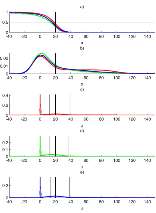
Results obtained for µb = 200, p0 = 0.5 and d = 100 are shown in Figure 1. Figure 1a

displays the computed (thick lines) and simulated (thin lines) estimates of P(H0|x),

while Figure 1b shows the estimates of the marginal density f(x). There is perfect agreement between simulated and computed estimates. The estimates of f(µ|x) are displayed for X = xobs = 80 in Figure 1c, 1d, 1e. They are all positive, the thick vertical

thick line at µ = 0 materializing the Dirac peak of area P(H0|X = xobs). There is still

excellent agreement between the computed and simulated estimates. In addition, for the three different priors under H1, we compared the simulated and computed

estimates of µ*, see Table 1. We checked the quality of the credibility interval by estimating its actual credibility level.

Estimates of µ* 95% credibility interval computed simulated computed actual

credibility level

Uniform 72.77 72.80 [34.23 ;98.35] 95.26 %

Exponential 65.27 66.17 [20.47 ;108.51] 95.36 % Half-Gaussian 67.20 67.58 [26.21 ;106.96] 95.26 %

Table 1. Validation of the results with mean dependant variance when µb = 200, p0 = 0.5,

d = 100, xobs =80.

The effect of lowering µb and xobs is shown in Figure 2, where µb = 50 (instead of 200)

and xobs = 20 (instead of 80), and as in Figure 1, p0 = 0.5, and d = 100. The

agreement between simulations and computations is still excellent, as also shown by Table 2. Interestingly, the Bayesian point estimate µ* of the true activity µ is systematically smaller than its classic counterpart (xobs), especially when xobs is not

much larger that than the standard deviation ) = (µ+2µb)1/2.

Estimates of µ* 95% credibility interval computed simulated computed actual

credibility level

Uniform 12.18 12.08 [0.00 ; 39.01] 95.46 %

Exponential 12.59 12.18 [0.00 ; 36.51] 96.13 % Half-Gaussian 13.31 13.11 [0.00 ; 38.36] 95.70 %)

Table 2. Validation of the results with mean dependant variance when µb = 50, p0 = 0.5,

Figure 1. µb = 200, p0 = 0.5, d = 100, xobs = 80 (thick vertical black line on all figures).

a) Computed (thick) and simulated (thin) estimates of P(H0|x) for the three priors under

H1: uniform (red), exponential (green), half-Gaussian (blue); the horizontal thin black line

materializes the a priori probability of H0, p0. b) Estimates of the marginal density f(x). c),

d), e): computed (thick) and simulated (thin) estimates of f(µ|X = xobs), prior $(µ|H1) (thin

dashed colored line), computed estimate of µ* and of the credibility interval (thin vertical black lines).

Figure 2. Same as in Figure 1 (p0 = 0.5, d = 100), but for µb = 50 instead of 200 and

xobs = 20 instead of 80.

The effect of having a smaller value of µb is that the posterior probability of H0 as a

function of x decreases faster to zero. However, having xobs much smaller increases

P(H0|X = xobs) and pushes the estimate of µ* towards zero. Note that the lower bound

4.2. Experimental results

4.2.1. Available records and pre-processing

Experimental records from twelve stations equipped with SAUNA detection systems [16] over a six-months period of daily measurements were studied, some stations being exposed to a low but steady radioactivity level (such as that of nuclear power plants (NPP) or medical isotope production facilities), others far from any known source of radioactivity. These stations detecting xenon fission gas are part of the CTBTO IMS that has been described in [18], and a map of their locations is available at www.ctbto.org/map#. The daily environmental observations provide records relative to the atmospheric concentrations of the xenon isotopes 131mXe, 133mXe,

133

Xe and 135Xe, and have been discussed in several publications [19-21].

More precisely, the records provide, for each isotope, the values of the net count, as well as Currie’s critical level and detection limit in Bq/m3, as defined in [1] and computed according to [16]. Thus, a first pre-processing step consisted in deducing the corresponding value of the blank count from these values. Second, prior to our analysis, the data went through a filtering step in order to ensure its good quality: state of health parameters describing the sampling and measurement conditions, (volume of air sampled, sampling and counting times) were checked to be within normal operating range. As a result, 7% of the available data was filtered out.

We present results pertaining to the 131mXe isotope. Due to its lower production rate and its longer half-life as compared to the other xenon isotopes, 131mXe exhibits the lowest concentrations that can be observed over long periods of time, and is hence a good example to illustrate the potentials of our approach for low-level measurements. Moreover, when analyzing a possible violation of the Treaty [22], a proven detection of this isotope would be important for two reasons: first, with its comparatively low yield when produced by the fission of uranium or plutonium [23], its detection - unless at extremely low concentrations compared to 133Xe - is rather indicative of fissions accumulated over time (like from operating NPP) as opposed to non-detectable concentrations (with minimal containment of a nuclear test) that would be released from the instantaneous fissions of a covert nuclear explosion; second, its presence may not only reveal a different fission scenario, but it is also a tracer of long term atmospheric transport, and a potential indicator of mixtures of air masses that need to be taken into account when ascribing consistent source terms and scenarios to the observations.

4.2.2. Checking for the Poisson distribution of the blank count

The results established in section 2 assume a constant blank count. In that case, the distribution of the blank should display a Poisson distribution. However, even for a

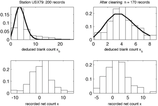
station with nearly constant blank, there may be outliers due to significantly different concentration levels or lower quality data that have escaped our first pre-processing step. Thus, we have performed a first fit of the (deduced) blank histogram by a Poisson distribution, and removed the values larger than its 99th percentile. After cleaning, half of the twelve stations display a Poisson or quasi-Poisson distribution. For these stations, the proposed framework is hence decided applicable. Figure 3 displays the results obtained for station USX79 (Hawai, USA): after cleaning, a second Poisson fit leads to an estimate value for µb of 4, with a 02 goodness of fit

p-value of 0.23, i.e. the density can be considered Poissonian.

Figure 3. Deduced blank count based data cleaning for station USX79 (decided Poisson distributed after cleaning). Top left: whole data set and first Poisson fit. Bottom left: corresponding recorded net counts. Top right: remaining data and second Poisson fit. Bottom right: remaining recorded net counts.

4.2.3. Estimation of the prior parameters

Thus, for the stations whose blank level µb can be assumed constant, we also have

available the cleaned histogram of the blank count, which is nothing else than the empirical marginal density f(x). The expressions of f(x) (A3), (A6) and (A9) with parameters p0 and d are fitted to the empirical histogram by maximum likelihood, i.e.

by minimizing minus the log likelihood function of the data –ln(L(p0, d)), with the

constraints that p0 ' [0, 1] and d $ 0. For each fit, in order to maximize the probability

to converge to the global minimum, 10 initializations of the two parameters are performed: the initial value of the estimate of p0 is chosen uniformly distributed in [0,

1], and the initial value of the estimate of d is chosen uniformly distributed in [0, 2 _µb],

fit on the cleaned data. For each initialization, the constrained optimization problem is solved by sequential quadratic programming [24].

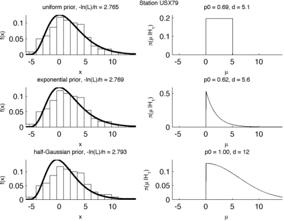
Figure 4. Prior fitting for station USX79 (with true blank considered constant). For each prior, the fit of the marginal density f(x) is on the left, and the corresponding estimate of the prior $(µ|H1) on the right.

Figure 4 shows the fits obtained for station USX79 with constant blank level estimated at _µb = 4, see previous section. The fit is visually much better with the

uniform and exponential priors than with the half-Gaussian prior, see also the values of the average cost –ln(L)/n after minimization on Figure 4. Both the uniform and the exponential priors agree on a prior probability of H0, i.e. of no radioactivity around

2/3, and therefore also on a small a priori level of radioactivity. These estimates are consistent with the station’s location far from any industrial source of xenon. Note that we verified that the Gaussian approximation holds for such small counts, see [3] for the exact density of the difference of two Poisson variables, and also [25] for a discussion of the validity of the Poisson-normal approximation.

4.2.4. Bayesian estimates and comparisons to other approaches

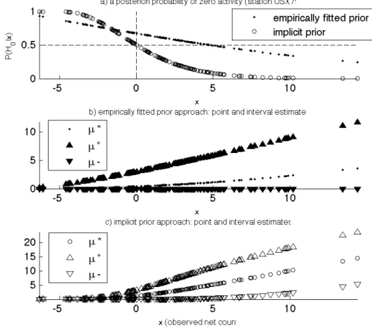
For each observed net count x at station USX79, we can estimate the posterior probability of zero radioactivity P(H0|x), the Bayesian estimate µ* for the true

radioactivity µ, and its credibility interval [µ– ; µ+]. For the computation of these estimates, we used the exponential prior which leads to a good fit of the marginal density. As stated previously, the estimate of P(H0|x), shown in Figure 5a, is not

available in the classic framework (and would even be meaningless), and the credibility interval, shown in Figure 5b, has the advantage with respect to the classic confidence interval not to include negative values. It is also interesting to note that the Bayesian estimate µ* of the true activity µ is much smaller than the classic estimate (simply equal to the observed count x). This effect was already noticeable in the simulated examples (see Table 1 and Table 2), though less strong because in these examples the observed x was larger as compared to its standard deviation (µ+2µb)1/2 than in the case of station USX79.

Figure 5. Bayesian estimates for station USX79 obtained with the exponential prior and the implicit prior approach: a) posterior probability of zero radioactivity P(H0|x) with both

approaches, b) point and interval estimates for the true net activity µ obtained with the exponential prior; c) estimates obtained with the implicit prior approach.

In order to illustrate the implicit prior approach proposed in [7], and to compare it to the proposed approach based on an empirically fitted prior, its results are also shown

in Figure 5. As depicted in section 3.1.2, even though the blank level is very small, the probability of no radioactivity automatically equals # for x = 0 (whereas the proposed approach makes an evaluation around 0.7). Point and interval estimates can be computed, but since the prior is implicit, the marginal density cannot be estimated nor related to any prior distribution of the radioactivity.

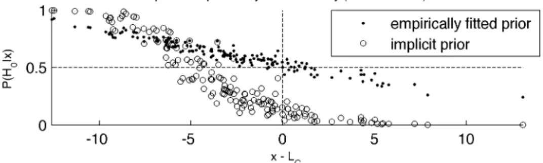
In order to make further comparisons with the classic decision framework, we can also plot the posterior probability estimate as a function of x – LC, where Currie’s

critical level LC = +11(1 – !) (2 xb)1/2 is computed with a type I error risk ! of 5%, see

Figure 6. In the classic framework, H0 is rejected if the observed count x exceeds LC,

hence in the right part of the graph. Interestingly, for this station, this coincides with the posterior probability of no radioactivity P(H0|x) being smaller than 1/2.

Figure 6. Same Bayesian estimate of the posterior probability of zero radioactivity P(H0|x)

as in Figure 5, but here as a function of x – LC, where LC is Currie’s critical level.

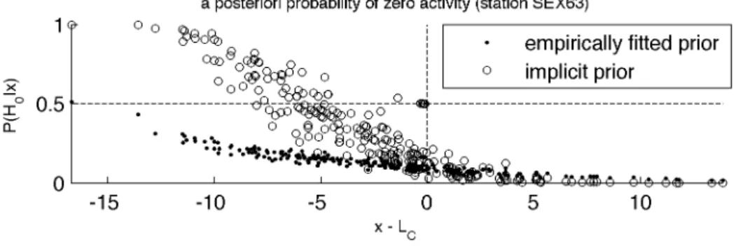
But the two approaches do not systematically coincide. Let us consider another station with quasi-constant blank level, SEX63 (Stockholm, Sweden). The true blank count µb is estimated at 6, and the exponential prior leads to the best fit, with a small

prior probability estimate of zero radioactivity of 0.13 and a maximum net count d = 7.1, i.e. a small net activity is very likely for this station. This is consistent with the station location in northern Europe, in the vicinity of NPPs. The posterior probability of no radioactivity P(H0|x) for this station as a function of x – LC is depicted in Figure

7. This time, with a threshold of 1/2 for P(H0|x), the proposed approach would detect

more radioactive events than the classic test.

However, in the Bayesian framework, the decision threshold should depend on the costs associated to the two types of error, as explained in section 2.2. It equals one half only in the case of equal costs. But if missing a real event costs more than a false alarm, the posterior probability does not need to be as small as 0.5 small in order to reject H0. This possibility to modulate the threshold is very appealing, but

also raises the difficult question of the quantification of the costs, the economic cost of analysts for the interactive study of the false alarms (CI), and the diplomatic cost of

Figure 7. Same as Figure 6, but for station SEX63.

The results of the implicit prior approach as a function of the classic ones are also given for both stations in Figure 6 (USX79) and Figure 7 (SEX63): the implicit prior approach detects more radioactive events than the classic framework for both stations. The interesting difference of behavior detected by the empirically fitted prior approach between a station far from any industrial source of radioxenon and one close to NPPs is not made clear by the implicit prior approach.

5. Discussion

Several points need to be discussed and/or further improved.

First, concerning the estimation of value of the background noise level µb, one could

think of including µb in the set of parameters to be estimated for the fit of the marginal

density, i.e. together with p0 and d, instead of estimating it separately from the

background measurements only. This is indeed a possibility, but it would deprive us from a means to detect undesired variations of µb, and to clean the data by removing

the corresponding outliers. As a matter of fact, we think that it is a quality of the method that, for each new observation, it requires first to test whether the observed xb is likely to be generated by a Poisson process with the estimated value of µb, and

that the answer be yes in order to apply the Bayesian scheme. Alternatively, if xb >> µb, one can still resort to the classic scheme. The possibility to deal with a

varying blank in a Bayesian framework is further discussed below.

Another reason not to include µb in the parameters to be estimated by the maximum

likelihood fit is that, for the moment, the goodness of the fit is not very well quantified by the value of the log-likelihood function, as pointed out for example in [26]. As a matter of fact, we used maximum likelihood estimation because the records that are available to us at the moment are too small to be able to work on binned data. In the case of sufficiently large data sets, it is possible to adjust the distribution via least squares on the binned data and, in that case, the goodness of the fit can be assessed through a 02 _{test. Thus, either we will dispose of much larger data sets in}

more satisfactory fashion. Larger data sets can already be obtained, but need so far time consuming interactive review to validate their quality.

A last point concerns the possibility of generalizing the proposed method to a varying blank level µb. This is theoretically feasible, but with some additional practical and

theoretical difficulties. First, the observed background signal xb will have to be

included in the Bayesian analysis; second, enough data should be available in order to be able to identify the joint marginal density of both net signal x and background signal xb. From the few practical results we already have, we feel that for many

stations, the background level will be either constant or take a few different values only, and that it is hence worth to test the proposed method as it is, but if necessary with the possibility to switch between several models, one for each level of µb.

6. Conclusion

In this paper, we have discussed a few approaches described in recent years to adapt Bayesian inference to the detection of low levels of radioactivity in the environment. With the help of mathematical considerations, we have pointed out the inherent drawbacks of these approaches and in particular the fact that they do not make the best use of the Bayesian notion of prior. In return, we have proposed and illustrated an innovative methodology that is closer to Bayesian principles and makes an extensive use of past environmental observations for prior estimation. This allows to analyze a new observation taking the available a priori knowledge into account, and to provide the probability for this observation to correspond to a truly radioactive sample, together with physically meaningful estimates of the true radioactivity value.

Appendix: Bayesian estimates for the proposed priors

In order to lighten the notations, the a priori probability of zero activity P(H0) is

denoted by p0 in the following results. According to (6), since f(x|µ) = 1/) *((x–µ)/)),

the a posteriori probability of H0 is always of the form:

P(H₀| x) = p₀ ! " x ! # $% & '( f(x) (A1)

According to (7), the posterior density of µ is always of the form:

f(µ | x) = P(H₀| x)!₀(µ) + (1" p₀)#(µ |H1) f(x) 1 $% x" µ $ & '( ) *+ (A2)

The marginal density f(x), the Bayesian point estimate (8), and the credibility interval (9) for µ are given below for the three priors.

A.1. Uniform prior

f(x) =p0 ! " x ! # $% & '(+ 1) p₀ d * x ! # $% & '() * x) d ! # $% & '( # $% & '( (A3)

Bayesian point estimate: µ* = !(1" p0) d# f(x) $ x ! % &' ( )* " $ x" d ! % &' ( )* % &' ( )*+ x + x ! % &' ( )* " + x" d ! % &' ( )* % &' ( )* (A4)

1 – & credibility interval:

µ+ = x +! " #$1 # d$ x ! % &' ( )* $ + 2 d" f(x) 1$ p₀ % &' ( )* µ$ = x +! " #$1 # d$ x ! % &' ( )* $ (1$ + 2) d" f(x) 1$ p₀ % &' ( )* if P(H0| x) < + 2,else µ $ = 0 , -. . / . . (A5)

A.2. Exponential prior

Marginal density with the exponential prior (14):

f(x) =p0 ! " x ! # $% & '( + 1) p₀ * xp !2 2*2 ) x * # $% & '(+ x)! 2 * ! # $ % % % & ' ( ( ( (A6)

Bayesian point estimate:

µ* = (1! p0) " # $ exp " 2 2$2 ! x $ % &' ( )* f(x) " 2₊ x!" 2 $ " % & ' ' ' ( ) * * *+ (x! "2 $ ), x!" 2 $ " % & ' ' ' ( ) * * * % & ' ' ' ' ( ) * * * * (A7)

1 – & credibility interval:

µ+ = x! " 2 # +" $ % !1 _1! & 2 # $ f(x) 1! p₀ exp x # ! "2 2#2 ' () * +, ' ( ) * + , µ! = x! " 2 # +" $ % !1 _{1! (1!} & 2) # $ f(x) 1! p₀ exp x # ! "2 2#2 ' () * +, ' ( ) * + , if P(H0| x) < & 2, else µ ! = 0 -. / / 0 / / (A8)

A.3. Half-Gaussian prior

Let us define 2 according to:

1 !2 = 1 "2 + 1 #2

Marginal density with the half-Gaussian prior (15):

f(x) = ! " x ! # $% & '( + ( ) ) * !+ " x + # $% & '(, * ! x # $% & '( (A9)

Bayesian point estimate:

µ* = 2(1! p0) "#f(x) $ x " % &' ( )* +3 x #2 , +x #2 % &' ( )*++ 2 $ +x #2 % &' ( )* % &' ( )* (A10)

1 – & credibility interval: µ+ = ! 2 "2 x +! # $ %1 _1% & 2 ' # " # f(x) 2!(1% p₀)( x / '

₍

₎

₍

₎

References

[1] L. A. Currie, Analytical Chemistry 335 (1968), 586.

[2] ISO 11929-7, Determination of the Detection Limit and Decision Threshold for Ionizing Radiation Measurements, Part 7: Fundamentals and General Applications (2005).

[3] W. E. Potter, Health Physics 76(2) (1999), 186.

[4] MARLAP Multi-agency radiological laboratory analytical protocols manual, vol. 20: detection and quantification capabilities (2004) [http://mccroan.com/marlap.htm]. [5] ISO 11929:2010(E) Determination of the characteristic limits (decision threshold,

detection limit and limits of the confidence interval) for measurements of ionizing radiation — Fundamentals and application, first Edition 2010-03-01 (2010).

[6] M. Zähringer, G. Kirchner, Nuclear Instruments and Methods in Physics Research A 594 (2008), 400.

[7] A. Vivier, Gilbert Le Petit, B. Pigeon, X. Blanchard, Journal of Radioanalytical and Nuclear Chemistry 282 (2009), 743.

[8] C. P. Robert. The Bayesian choice: from decision-theoretic motivations to computational implementation. Springer 2nd ed (2001).

[9] T. Leonard, J. S. J. Hsu. Bayesian methods: an analysis for statisticians and interdisciplinary researchers. Cambridge University Press (1999).

[10] P. Donnelly, Significance 2(1) (2005), 46.

[11] CTBT. Text of Comprehensive Nuclear-Test-Ban Treaty (1996). See Web Page of the United Nations Office for Disarmament Affairs (UNODA), Multilateral Arms

Regulation and Disarmament Agreements, CTBT

[http://disarmament.un.org/TreatyStatus.nsf].

[12] W. Hoffmann, R. Kebeasy, P. Firbas, Physics of the Earth and Planetary Interiors 113 (1999), 5.

[13] M. Zähringer, A. Becker, M. Nikkinen, P. Saey, G. Wotawa, Journal of Radioanalytical and Nuclear Chemistry 282 (2009), 737.

[14] J. P. Fontaine, F. Pointurier, X. Blanchard, T. Taffary, J. Environ. Radioact. 72 (2004), 129.

[15] G. Le Petit, P. Armand, G. Brachet, T. Taffary, J. P. Fontaine, P. Achim, X. Blanchard, J. C. Piwowarczyk, F. Pointurier, Journal of Radioanalytical and Nuclear Chemistry 276 (2008), 391.

[16] A. Ringbom, T. Larson, A. Axelsson, K. Elmgren, C. Johansson, Journal of Radioanalytical and Nuclear Chemistry A 508 (2003), 542.

[17] Y. V. Dubasov, Y. S. Popov, V. V. Prelovskii, A. Y. Donets, N. M. Kazarinov, V. V. Mishurinskii, V. Y. Popov, Y. M. Rykov, N. V. Skirda, Instrum. Exp. Tech. 48 (2005), 373.

[18] J. Schulze, M. Auer, R. Werzi, Applied Radiation and Isotopes 53 (2000), 23. [19] M. Auer, A. Axelsson, X. Blanchard, T. W. Bowyer, G. Brachet, I. Bulowski, Y.

Dubasov, K. Elmgren, J. P. Fontaine, W. Harms, J. C. Hayes, T. R. Heimbigner, J. I. McIntyre, M. E. Panisko, Y. Popov, A. Ringbom, H. Sartorius, S. Schmid, J. Schulze, C. Schlosser, T. Taffary, W. Weiss, B. Wernsperger, Appl. Radiat. Isotopes 60 (2004), 863.

[20] T. J. Stocki, X. Blanchard, R. D’Amours, R. K. Ungar, J. P. Fontaine, M. Sohier, M. Bean, T. Taffary, J. Racine, B. L. Tracy, G. Brachet, M. Jean, D., Meyerhof, J. Environ. Radioact. 80 (2005), 305.

[21] P. R. J. Saey, C. Schlosser, P. Achim, M. Auer, A. Axelsson, A. Becker, X. Blanchard, G. Brachet, L. Cella, L.-E. De Geer, M. B. Kalinowski, G. Le Petit, J. Peterson, V. Popov, Y. Popov, A. Ringbom, H. Sartorius, T. Taffary, M. Zähringer, Pure Appl. Geophys. 167 (2010), 499.

[22] A. Ringbom, K. Elmgren, K. Lindh, J. Peterson, T.W. Bowyer, J.C. Hayes, J.I. McIntyre, M. Panisko, R. Williams, Journal of Radioanalytical and Nuclear Chemistry 282 (2009), 773

[23] T. R. England, B.F. Rider, Los Alamos National Laboratory, LA-UR-94-3106, ENDF-349 (1993).

[24] R. Fletcher. Practical methods of optimization. Wiley, 2nd edition (1987).

[25] L. A. Currie, Journal of Radioanalytical and Nuclear Chemistry 276 (2008), 285. [26] J. Heinrich, Pittfals of Goodness-of-fit from likelihood. PHYSTAT2003, SLAC,