Coupling partial-equilibrium and dynamic biogenic carbon models to assess future transport scenarios in France

(1)

HAL Id: hal-02051920

https://hal-ifp.archives-ouvertes.fr/hal-02051920v2

Submitted on 19 Mar 2019

HAL is a multi-disciplinary open access archive for the deposit and dissemination of sci-entific research documents, whether they are pub-lished or not. The documents may come from teaching and research institutions in France or abroad, or from public or private research centers.

L’archive ouverte pluridisciplinaire HAL, est destinée au dépôt et à la diffusion de documents scientifiques de niveau recherche, publiés ou non, émanant des établissements d’enseignement et de recherche français ou étrangers, des laboratoires publics ou privés.

Coupling partial-equilibrium and dynamic biogenic

carbon models to assess future transport scenarios in

France

Ariane Albers, Pierre Collet, Daphné Lorne, Anthony Benoist, Arnaud Hélias

To cite this version:

Ariane Albers, Pierre Collet, Daphné Lorne, Anthony Benoist, Arnaud Hélias. Coupling partial-equilibrium and dynamic biogenic carbon models to assess future transport scenarios in France. Ap-plied Energy, Elsevier, 2019, 239, pp.316-330. �10.1016/j.apenergy.2019.01.186�. �hal-02051920v2�

(2)

Coupling partial‐equilibrium and dynamic biogenic carbon models

to assess future transport scenarios in France

Ariane Albers 1,2,3,*, Pierre Collet 1, Daphné Lorne 1 , Anthony Benoist 3,4, Arnaud Hélias 2,3,5

1_{IFP Energies nouvelles, 1 et 4 Avenue de Bois‐Préau, 92852 Rueil‐Malmaison, France.} 2 _{LBE, Montpellier SupAgro, INRA, UNIV Montpellier, Narbonne, France.} 3_{Elsa, Research group for Environmental Lifecycle and Sustainability Assessment, Montpellier, France.} 4 _{CIRAD ‐ UPR BioWooEB, Avenue Agropolis, F‐34398 Montpellier, France.} 5 _{Chair of Sustainable Engineering, Technische Universität Berlin, Berlin, Germany.} * Corresponding author. Phone: +33 (0) 7 89 04 71 25, E‐mail: ariane.albers@ifpen.fr

Abstract

Bioenergy systems are promoted in an effort to mitigate climate change, and policies are defined accordingly to be implemented in the coming decades. Life Cycle Assessment (LCA) is used to assess the environmental performance of bioenergy systems, yet subject to the limitations of static approaches. In classical LCA, no temporal differentiation is undertaken: all inventoried instant to long‐term greenhouse gases emissions (GHG) are aggregated and characterised in the same way, over a fixed time horizon, by means of fixed characterisation factors. Positive and negative impact contributions of dynamic biogenic carbon (Cbio) sum up to zero, yielding the same result as carbon neutral estimates. Climate mitigation

results are biased without the temporal consideration of these flows. The purpose of the study is to highlight the time‐sensitive potential climatic consequences of policy‐driven transport strategies for metropolitan France, in the specific context of the dynamic LCA framework and climate change mitigation. We therefore propose a dynamic approach coupling a partial‐equilibrium model (PEM) with dynamic Cbio models. The PEM analyses in detail the techno‐economic performance of the metropolitan French energy‐ transport sector. It explores prospective optimisation options (supply‐demand equilibrium) of emerging commodity and energy process pathways in response to a policy in question. The Cbio model generates

dynamic inventories of the Cbio embedded in the primary renewable biomass outputs of the PEM. It

captures the dynamic Cbio exchange flows between the atmosphere and the technosphere over time:

negative emissions from fixation (sequestration) and positive emissions from release (e.g. combustion or decay). A dynamic impact method is applied to evaluate the mitigation effects of Cbio from forest wood

residues by comparing the climate change impacts from complete carbon (fossil + biogenic) with carbon neutral inventories across scenarios. Two sets of results are computed concerning the overall transport (all emissions) and bioethanol (wood‐to‐fuel emissions) systems. The mitigation effect from long‐term historic sequestration allocated to bioethanol (462%) is significantly larger than for transport (3%), expressed as the difference with carbon neutral estimates. The fossil‐sourced emissions from bioethanol production represents only 5.4%. In contrast, a comparison with an alternative reference scenario involving wood decay demonstrated higher impacts (i.e. an increase of 316%) than carbon neutral estimates. The representation of the actual climatic consequences depends on the chosen fixed end‐year of the dynamic impact assessment. Moreover, the mitigation effect is proven sensitive to the rotation length of forestry wood: the shorter the length the lower the mitigation from using renewable forest resources. Other energy‐policy scenarios, Cbio modelling approaches and consequences of indirect effects should be further

studied and contrasted.

Keywords: biogenic carbon from renewable resources, climate change mitigation, time‐dynamic life cycle assessment, transport sector, partial‐equilibrium model.

(3)

Acronyms

1G First generation 2G Second generation BAU Business‐as‐usual C Carbon Cbio Biogenic carbon CF Characterisation factor CH4 Methane gas CLCA Consequential life cycle assessment CO2‐eq Carbon dioxide equivalent EC‐JRC European Commission Joint Research Centre FoWooR Forest wood residues GHG Greenhouse gases GWP Global warming potential IPCC International Panel on Climate Change LCA Life cycle assessment LCG Lignocellulosic LCI Life cycle inventory LCIA Life cycle impact assessment MARKAL Market Allocation N2O Nitrous oxide PEM Partial‐equilibrium model TH Time horizon TIMES The Integrated Markal‐Efom System

(4)

1 Introduction

The energy sector is the main contributor to global anthropogenic greenhouse gas (GHG) emissions [1]. In France, energy for transport is the principal emitter, accounting for almost one‐third of the national emissions[2]. Policy planning faces the challenge of responding to climate change threats and secure future energy supply. Ambitious political targets enforce transitioning into renewable resources and increased energy efficiency, to limit temperature rise to 1.5 to 2 degrees Celsius [1]. The French Energy Transition for Green Growth Act), adopted in 2015, directs the energy sector towards low‐carbon strategies and multi‐ annual energy programs [2]. France anticipates major renewable shares in the transport sector ─aimed at mitigation of GHG emissions─ gradually increasing up to the year 2050. Energy modelling has become a key instrument to inform robust decision‐making in energy system planning [3]. A wide variety of prospective models have emerged in the last half‐century to support multilateral cooperation in macroeconomic energy system analysis. Top‐down general‐equilibrium models analyse the energy systems of a whole economy to identify cross‐sectoral substitution alternatives [4]. In contrast, bottom‐up partial‐equilibrium models (PEM) analyse in detail the techno‐economic performance of single energy sub‐sectors [5,6]. Among the most used model generators featuring detailed technology databases are the MARKAL (MARKet ALlocation) and TIMES (The Integrated Markal‐Efom System) of the International Energy Agency’s Energy Technology System Analysis Program [7–9]. More recently, hybrid models combine economy‐wide perspectives with neoclassical growth models, sectoral and technological details [10,11]. Coupling with macroeconomic models at global scales, in the view of decarbonisation mechanisms to internationalise environmental externalities, is commonly discussed in climate change abatement efforts [8]. Biofuels are promoted as low carbon energy carriers to meet climate change and energy policy targets. However, these substitution alternatives have been questioned in the past. Environmental and social concerns have arisen from expanding food crop based biomass (e.g. corn, wheat, rapeseed), particularly concerning land use and food security [12–16]. Dedicated or residual lignocellulosic biomass (e.g. forest wood, agricultural straw, miscanthus) are non‐food alternatives to energy crops feeding a wide range of emerging energy pathways for heat, electricity or transport fuels. Techno‐economic and environmental research has been conducted linked to bioenergy from innovative biomass supply chains, for instance, from forest wood residues [17–19], crop‐residues [20–22], and miscanthus [23,24]. Advanced transport biofuels, from dedicated or residual lignocellulosic biomass, are under development to partially substitute petroleum fuels [25]. From 2020 onwards, it is expected that second generation (2G) biofuel pathways will generate cellulosic ethanol and Fischer‐Tropsch biodiesel, at commercial scales, competitive with conventional fuels [26–28]. Life Cycle Assessment (LCA) is widely used to assess the climate change impacts and other potential environmental effects of bioenergy systems. Several bioenergy LCA studies have been carried out concerned with lignocellulosic biomass for electricity and heat generation, as reviewed by Muench and Guenther [29]. LCA has been increasingly combined with PEM in consequential LCA (CLCA) studies [30–37]. CLCA quantifies the environmental burden, and its variation, associated with changes in demand, often driven by policy decisions, beyond the boundaries of a particular production system [38]. It studies how flows change in response to a prior (retrospective) or future (prospective) decision [39]. The environmental consequences of a change in bioenergy systems are linked with expansion, displacement [40,41] or intensification [40,42].Combined LCA and PEM has been applied to assess the prospective consequences of emerging markets (advanced commodity and bioenergy pathways), to estimate how future decisions would change material and energy flows. Menten and colleagues applied the French TIMES‐MIRET model to

(5)

improve consistency in prospective CLCA studies of biofuels and biomass‐to‐liquid processes [31].

Levasseur and colleagues used the Canadian TIMES NATEM model and complemented its outputs with LCA of alternative butanol from forest biomass pathways [30].

However, combined LCA and PEM approaches are usually static. The assessment of GHG emissions, for instance, focus on fossil fuels, while disregarding the time‐sensitive climate change effects of biogenic carbon (Cbio) embedded in biofuels. Cbio refers to the carbon fixed in the biomass/plant resource through

photosynthesis. The Cbio is temporally sequestered and stored in biomass and released back to the

atmosphere at the end‐of‐life (e.g. through combustion or decay). The climate change impact category is based on the IPCC Global Warming Potential (GWP) metric [43]. The GWP method represents the weighted sum of all GHG emissions, such as carbon dioxide (CO2), methane (CH4) and nitrous oxide (N2O), over a 20

or 100‐year time horizon (TH), relative to the CO2 reference gas, computed by means of characterisation

factors (CFs). The GHG emissions are then expressed per functional unit of a product or service (e.g. per km driven by an average passenger car). This static method disregards the time dimension affecting climate change results [44–51]. In other words, GHG emissions are not differentiated through time.

The exclusion of dynamic Cbio elementary flows in the GHG inventories is justified by the carbon neutral

hypothesis. This simplification, based on the classical static approach, balances out the sequestration and release flows through the weighted sum of all emissions at time zero [52–54]. The bio‐sourced GHG emissions, thus, yield zero climate change impact. However, this static methodological choice has been challenged for biomass resources with long rotation lengths, particularly from forestry [53,55,56]. Long CO2 (re‐)sequestration periods (e.g. forest trees) have time‐sensitive effects, whereby rotation lengths lower than one‐year (e.g. annual crops) may have small to zero impacts (equivalent to carbon neutral estimates) [57,58]. Long‐term carbon stocks (e.g. forest trees) have a negative atmospheric impact, however they are reversible (i.e. reemitted) at some point in time, making it highly debatable whether or not assigning a value to it is justifiable [59,60]. Non consideration of long‐term Cbio sequestration and the timing of this

emissions release thus produce biased results [61]. In the last decade, new dynamic LCA approaches have emerged focused on time‐sensitive climate change effects from bioenergy [46,47,50,56,62–64], and more specifically, linked to biogenic carbon accounting and forest resources [63,65–70]. Cherubini and colleagues proposed the biogenic global warming potential (GWPbio) metric for bioenergy systems, using the impulse response function [71], to predict the biogenic CO2 decay, as a function of biomass rotation dynamics [56]. The factors assign lower impacts to fast‐ growing vegetation and vice‐versa. Yan developed CFs for different rotation lengths and harvest intensities based on forest‐specific carbon cycle models [72]. The dynamic LCA method by Levasseur and colleagues enables assessing temporal emission profiles of fossil or biogenic flows, as a function of time [47]. The dynamic method computes time‐dependent CFs for any year following an emission. It’s application requires dynamic inventories, differentiating each emission flow from and to the atmosphere through time. Time‐ explicit Cbio inventories of forestry resources have been proposed by De Rosa and colleagues, through a

simplified parametric model for aboveground and belowground forest carbon stocks [67]. To this day, no consensus exists on how to model dynamic Cbio inventories from renewable resources.

The purpose of this study is thus to assess, ex‐ante, the time‐sensitive potential climatic consequences of policy‐driven transport strategies for France, by means of a full carbon accounting approach. We propose the coupling of a techno‐economic and biogenic carbon models in the specific context of the dynamic LCA framework and climate change mitigation. The novel model coupling bridges the gap between research, development of emerging bioenergy systems and their actual mitigation effects.

(6)

2 Material and method

The proposed model‐coupling of the PEM and the dynamic Cbio model is shown in Fig. 1. The overall

coupling strategy is as follows: The renewable commodity forest wood residues (hereafter referred as FoWooR), described by the PEM, is selected for the first coupling attempt. The dynamic biogenic carbon is assessed through a Cbio modelling tool developed for this coupling strategy. It models the dynamic Cbio

exchange between the atmosphere and the technosphere over time: negative emissions from fixation (sequestration) and positive emissions from release (e.g. combustion or decay). The model generates dynamic inventories of the Cbio embedded in the renewable FoWooR biomass (hereafter referred to as Cbio

balance. For the climate change impact assessment, a dynamic method is applied to compare the climatic consequences of carbon neutral (without Cbio: hereafter referred to as “C neutral”) and complete carbon

balances (with Cbio: hereafter referred to as “complete C”) in response to policy scenarios. The complete C

balance is built upon both fossil and biogenic material and energy flows from production and consumption of petroleum fuels and biofuels, while the C neutral approach accounts for the fossil ones only. The coupled model thus produces a dynamic climate change impact assessment of prospective renewable biomass and energy pathways driven by and representing policy decisions. All necessary steps for the model coupling are detailed in this section, following the classical LCA steps: goal and scope, life cycle inventories (LCI), and life cycle impact assessment (LCIA). Fig. 1. Conceptual diagram of the model coupling strategy of the TIMES‐MIRET partial‐equilibrium model with dynamic biogenic carbon modelling 2.1 Goal and scope: temporal boundaries The goal of the present study is to highlight the time‐sensitive potential climatic consequences of policy‐ driven transport strategies for France. The system boundary is the transport sub‐sector, with special focus on 2G biofuels. Energy services from electricity and heat for other end‐users (e.g. industrial, domestic) are excluded from the study. The Cbio balance represents the supply of FoWooR, as a primary renewable

(7)

resource for biofuel production. The LCIA is based on time‐dependent CFs [47] and is expressed here in mega‐tonnes of carbon dioxide equivalent. Other LCA environmental impact categories are outside the scope of the study, as the main focus is the time sensitive clime change impact assessment of dynamic Cbio flows and its comparison with C neutral approaches. The dynamic LCA approach, aims at developing a dynamic complete C balance (fossil + biogenic emissions). Therefore, the temporal differentiation of all emission flows, particularly of biogenic origin, is a fundamental precondition. The temporal system boundary requires all necessary time specifications of the entire study under assessment, namely the time step as well as both the LCI time horizon (LCI TH) and the LCIA time horizon (LCIA TH), specified below. The time step defines the temporal frequencies over which the emissions are inventoried and assessed (e.g. per minute, hour, day or year). It is set by the inherent time scales of the impact categories [73,74]. Inherent features of impact categories (e.g. climate change, acidification, eutrophication, etc.) relate to several biogeochemical processes, defining the temporal resolution at which dynamic inventories can be modelled. LCA methods encompass different impact categories, however the present study is only concerned with climate change category. For this impact category, the time scale of the flows is recommended at annual frequencies [47,75]. Therefore, the dynamic computation of the technical flows and elementary flows are modelled on an annual basis. The LCI TH defines the timeline over which the GHG emission are considered in the study, describing each emission flow through time. We perform a full‐time inventory of all GHG emission with no temporal cut‐ offs. Since the model‐coupling in this study aims at assessing the PEM outputs, the negative and positive flows are aligned with the TH of the PEM simulation. TIMES‐MIRET runs over multiple‐periods (3 to 5 years) until the year 2050. For this study the PEM outputs from 2019 to 2050 are taken into consideration. A linear‐interpolation is performed to track the multi‐period outputs on an annual basis and develop annual values for the dynamic inventories. The LCI TH of all negative emission flows is defined by the chosen modelling approach taking into account historic or future Cbio fixation time perspectives (described in

section 2.3.1).

We inventoried the Cbio sequestration flows before the final harvest of FoWooR (historic perspective). A full

rotation length accounts for 200 years in this study. The long‐sequestration period follows [76], as detailed in section 2.3.1. It represents all main tree species of the French wood industry, with Sessile Oak (Quercus petraea) having the longest sequestration length. For the historic Cbio computation, the TH of the PEM

simulation represents the last year of the Cbio fixation, at which final harvest of FoWooR occurs. For

instance, for the period 2019‐2050, the first fixation flow starts 200 years in the past (year 1819) for the year 2019, 1820 for the year 2020 and so forth until 1850 for the last simulation year (2050). The LCIA TH, likewise, defines the period over which the climate change impact is considered by means of setting a fixed reference year or an end‐year of the impact assessment. The commonly use TH for the climate change characterisation in LCA is one century, as per the default GWP metric [43,77,78]. We therefore fix a future reference year to 2119, 100‐years after the first PEM simulation year (2019). Yet, any end‐year or TH can be chosen when dynamic LCIA is performed with time‐dependent CFs. Finally, the temporal system boundary for the entire study under assessment can be described. The annual time step consideration of a full‐time accounting approach with historic fixation flows and a fixed future reference year, sets the overall temporal system boundary over the period 1819 to 2119: 300 years in total. This temporal specification provides transparency and allows a systematic comparison among all assessed PEM policy scenarios. Moreover, the selected period represents consistency between the LCI and the LCIA

(8)

TH, with no temporal cut‐offs. Accordingly, we ensure that all inventory flows are projected over the same TH into the future. 2.2 Life cycle inventories: partial‐equilibrium model outputs 2.2.1 Description of the key elements The economic partial‐equilibrium model used in this study is the TIMES‐MIRET, adapted to the modelling framework from the MARKAL/TIMES family of models [7–9]. TIMES‐MIRET analyses the energy‐transport system of metropolitan France over a multiple‐period horizon based on prospective demographic and economic projections [79]. The model conducts a detailed bottom‐up techno‐economic analysis, describing the primary resource supply (petroleum fuels and biomass), its transformation to secondary fuels via different process pathways (refinery), and the final energy consumption (electricity, heat and transport fuels) [8,79]. Petroleum‐ and biomass‐based commodities represent the supply of energy sources to meet the future energy demand. Each source has an attribute, detailing the availability/import, capacity and marginal cost. The demand curve is represented by the energy services in transportation (automobiles, trucks, rail, aviation), domestic and commercial (space heating, lightning, cooling), industry (chemicals, steel) and agriculture segments [9]. In TIMES‐MIRET the assessed useful energy includes electricity and heat (hereafter referred to as “energy mix”), and transport fuels (hereafter referred to as “transport sub‐ sector”). The output from the supply‐demand equilibrium assumes a perfectly competitive market, in which producers and consumers maximise their net total surplus or minimise their net total costs, while meeting several (policy) constraints [5,9]. The TIMES‐MIRET PEM scenario simulations disregard cross‐sectoral interactions within a whole economy (in contrast to general‐equilibrium models). However, each scenario explores the linear programming optimisation of supply‐demand in detail based on a technology‐explicit database linked with different commodities. For instance, for the transport sub‐sector the functional unit of the sectoral output is the kilometres travelled by a specific transportation means (e.g. average passenger car, heavy trucks, etc.). In bottom‐up PEM models, the existing and future technologies to produce that given unit are explicitly specified [9]. 2.2.2 Definition of policy scenarios TIMES‐MIRET outputs are scenario‐dependent. The assessed policy scenarios are compared with a reference policy scenario (business‐as‐usual, BAU). The BAU scenario represents a baseline against which alternative policy scenarios are compared. BAU is formulated from historical and established norms considered valid until the end of the PEM simulation TH. The reference policy draws back to the 2009 EU Directive and National Renewable Energy Action Plan, pursuing renewable energy targets in the gross final energy consumption by the year 2020. Therefore, the initial period of the TIMES‐MIRET is calibrated to the year 2009, fixing the historic values and main variables, yet considering changes in future demand. The alternative policy scenario assessed in the present study is named 15Bio. It corresponds to the national long‐term, multiannual energy transition plan, partly formulated from the French Energy Transition for Green Growth Act. For the 15Bio scenario, we adopted the 15% RE share in the transport sub‐sector by 2030, in reference to the year 2012. This specific target for the transport sector was subjected to the EU Renewable Energy Directive, legally binding Member States to increase the RE share in addition to limiting food crop‐based biofuels (first generation, 1G) to 7% by 2020. For the French national energy plan, this target remains effective up to the year 2030. Hence, the 15Bio scenario involves all constraints of the BAU reference, including the new set of policies (i.e. limiting 1G biofuel share to 7% and increasing the

(9)

renewable energy share by 15% by 2030). A comparison with the BAU scenario, allow identifying the policy‐ induced consequences of energy‐transport pathways in response to fossil fuel and energy‐crop substitution targets to mitigate climate change. 2.2.3 Selection of the model outputs In the LCA context, the PEM commodities represent the technical flows, while all life cycle carbon and GHG emissions the elementary flows. For the model coupling, the technical and elementary flows of the PEM are exported per BAU and 15Bio policy scenarios. All flows associated with the transport sub‐sector are separated from the pathways for other end‐users. For instance, cogeneration processes (heat and electricity generation) and biochemical or thermo‐chemical processes (bioethanol production) are both linked to FoWooR commodity in the 15Bio scenario. For the present study, we exclusively focus on the pathways associated with transport fuels only.

Concerning the technical flows for modelling Cbio inventories, the selection of the biomass commodity

followed two main criteria: lifespan of the vegetation with a full rotation length longer than one year and contribution to 2G transport biofuels. FoWooR is an energy carrier with mid‐ to long‐term sequestration periods, and under the new set of policies, it is expected to contribute to 2G bioethanol with mayor shares. Annual crops are excluded from the Cbio modelling, as their Cbio fixation‐release dynamics occur within one

year (equivalent to carbon neutral approaches), thus no climate change impact is estimated. Other long‐ lived renewable biomass resources, such as short‐rotation coppices or perennial crops, could have been modelled to included their Cbio balances in the dynamic GHG inventories. However, their contribution to 2G

biofuels is comparatively small or absent in the 15Bio scenario, and thus negligible for the Cbio analysis

under the assessed 15Bio policy scenario. The PEM input data for FoWooR in the 15Bio policy scenario is based on national forest inventories for the French wood supply chain and a roadmap 2035 study made about the future availability of this renewable resource in France [80]. The prospective assumptions consider, among others, harvest losses amounting 8% for merchantable wood, 15% for merchantable and residues, and 50% when FoWooR are harvest separately [80].

Regarding elementary flows for modelling carbon neutral GHG inventories, fossil‐based CO2 and N2O

elementary flows are provided by the PEM associated with all production and consumption pathways: biomass cultivation, transportation, (bio‐)refinery, industry, tailpipe, and trade. However, all elementary flows of the transport‐pathways are re‐calculated, using the updated emission factors of the European Commission Joint Research Centre (EC‐JRC) based on the JEC Well‐To‐Wheels (WTW) method [81]. The emission factors are expressed in equivalent CO2 emissions per MJ petroleum‐ or biomass‐sourced fuels. To recalculate the CO2‐equivalent values into the respective GHG elementary flows, the values are divided by

the IPCC GWP equivalent factors [43]. The proportions of the CO2, N2O and CH4 GHG emission per specific

fuel are also taken from the EC‐JRC [81]. The fossil‐sourced elementary flows from the transport sub‐sector are combined with the biogenic‐sourced flows to develop a complete C balance and compare its climate change impact with C neutral approaches.

2.3 Life cycle inventories: biogenic carbon model outputs

The technical flow (i.e. the FoWooR commodity) is coupled with the Cbio models to compute time‐explicit

Cbio inventories. The mass of FoWooR is expressed in Cbio by means of a wood‐specific carbon content

factors (0.4952) denoting the weighted mean of all assessed forest tree species of the French wood supply chain assessed in Albers et al.(in press). The Cbio elementary flows represent the Cbio embedded in the

(10)

primary FoWooR supply flows per tonne of FoWooR [t of Cbio]. The coupling with dynamic Cbio models

further generates annual fixation and release flows. The dynamic Cbio balance is converted into biogenic CO2

and CH4 for the impact characterisation by multiplying the molecular weight of CO2 or CH4 to the atomic

substance of C (44/12) or (16/12) respectively. CH4 is considered for decay estimates only [82–84]. or the Cbio balance, the belowground tree compartment (roots and stump) is also considered, to include both aboveground and belowground Cbio dynamic. This implies allocating a proportion of belowground biomass to the FoWooR. The aboveground compartment represents about 80% of the tree (63% stem and 37% FoWooR). 20% of the tree consists of belowground biomass, as computed with our Cbio modelling tool. The values are congruent with other studies (e.g.[85]). The allocation factor for the belowground biomass corresponding to FoWooR was estimated at 0.25 of FoWooR, which represents 7.4% of the total tree biomass. 2.3.1 Computation of carbon fixation from forestry resources

Fixation represents the withdrawal of CO2 from the atmosphere due to photosynthesis. The dynamic Cbio

modelling of the FoWooR applied dynamic growth models from forestry science, elaborated for the French forest wood industry. The modelled data supports and informs dynamic modelling approaches to predict mean growth and Cbio fixation dynamics of a tree or forest stand over a given rotation length. All data and

modelling steps for the Cbio fixation flows were obtained from yield tables per unit area of forest stands,

non‐linear growth models and allometric relations (see Table 2 in Albers et al. in press). The tabulated yield table data based on empirical evidence originated from long‐standing experimental forest plot surveys of managed forests throughout France [86] or other regions when not available for France [87,88]. The non‐ linear growth curve is represented by the often used Chapman‐Richards (CR) model, a sigmoid and asymptotic curve [89–91]. The CR equation (Eq. 1) expresses the potential growth of a tree species in height and diameter‐breast‐height or circumference (response growth variables) at age (independent variable), with species‐ and site‐dependent parameters , , , [92]:

1 ε Eq. 1

with 1/ 1

For the Cbio fixation dynamics, we used annual stocking values from all assessed tree species (Table 2 in in

Albers et al. in press) and the weighted mean based on the standing wood production volumes and distribution from national statistics and surveys [93] (see Table 3, 5 and 6 in Albers et al. in press). The annual stocking factors are expressed in tonnes of Cbio. Note that, the dynamic Cbio fixation model represent

monospecific (individual‐species) uneven‐aged forest stands with homogenous growth. Other site‐ dependent dynamic elements related with, for instance, mixed forest stands (two or more species per forest stand), and losses from mortalities, including those unexpected due to natural events (e.g. wildfires, diseases, winds) and soil organic carbon, were not modelled. For modelling site or case‐specific fixation dynamic, these site‐specific parameters would further complement and improve dynamic approaches. For the computation of Cbio fixation, two time‐dependent accounting approaches can be followed for the

first Cbio fixation flow: a) a full rotation length starting after the wood‐use, in the same year of final wood

harvest, when trees are removed from the forest stand and new seedlings are re‐planted; or b) a full rotation length starting before the wood use. The former refers to Cbio fixation flows with future timelines

and the latter to historic ones. In previous LCA studies, future [56,67,94], historic [95–97], and both

[66,98,99] Cbio fixation time perspectives were tested. In the present study, we computed Cbio fixation flows

with historic timelines. The reasoning behind this modelling approach is based on the assumption that the provision of FoWooR as biofuel feedstock is retained from sustainably managed forests in the French/EU

(11)

context. According to Lindeijer and colleagues, the origin of the biotic resource defines whether the modelled systems is man‐made controlled or a natural ecosystem [100].

The biogenic carbon fixation dynamic [t Cbio. y‐1] is defined by:

, Eq. 2 , . 1 Eq. 3

where the relative biogenic carbon fixation expressed in tonnes, , is the carbon fixation model with a set of parameters of the Chapman‐Richards model (p), τ (y) is the time variation between the start time ( ) of the biogenic carbon fixation and the cutting time ( ) defined by each thinning and a final cut time (i.e. harvest at the end of the rotation length).

The coupling with the partial‐equilibrium model is carried out following Eq. 4 and Eq. 5, where is the total biogenic carbon, ∗_{is the biogenic carbon output from the partial‐equilibrium model, expressed in}

tonnes, at a given time ∗. The fixation dynamic at ∗ is computed following the computation in Eq. 6:

∗ Eq. 4 with t the a time of the MIRET scenario and ∗ _∗ _Eq. 5 Thus, ∗ , ∗ , ∗ _∗ Eq. 6 2.3.2 Computation of carbon release from forestry products

The Cbio release to the atmosphere is positive, because it contributes to the atmospheric GHG

concentration and thus to the radiative forcing effect. The flow occurs when the Cbio is emitted back at the

EOL of the biomass product. For bioenergy systems, the EOL is the combustion process. EOL combustion of bioenergy is linked with internal combustion engines (transport tailpipe) or cogeneration processes (energy mix). In the present study, it is assumed that the biomass is harvested, processed and used within the same year. This means that the total embedded Cbio in the FoWooR, including co‐products and wastes, is emitted

back to the atmosphere within the same year of harvest.

However, when the residual part from logging operation are not used for the bioenergy market (e.g. 2G bioethanol), they are left in the forest. The alternative EOL pathway corresponds to a reference scenario in which FoWooR are left behind and excluded from economic activities. For comparison purposes, the selection of an adequate reference systems was already highlighted by other authors [106,107]. For the

(12)

alternative EOL pathway, the left behind FoWooR are subjected to onsite natural decay processes by microbes in the soil in forest ecosystems. After harvest aboveground residues and belowground biomass are assumed to decay completely over time [101]. Emissions due to decay occur over long periods of time, gradually decreasing towards zero. The decay curve of residual dead wood biomass can be estimated via a first‐order exponential decay equation (Eq. 1), where is the remaining mass at time , the initial dry mass, and τ is the half‐life estimates.

/ _Eq. 1

The negative exponential decay model is commonly used and recommended to estimate forest wood degradation [19,21,102,103]. Half‐life values for decay vary depending on the tree compartment. For τ we used eight years for coarse woody debris and thirty years for dead stumps and roots [104]. A part of the embedded Cbio in FoWooR is emitted as CH4 (due to anaerobic degradation), ranging between 0% and 3%

(we used 1.5%) for coarse woody debris (branches, twigs and foliage) and 10% for belowground dead stumps and roots [105]. The CH4 releases are very uncertain and site‐dependent. CH4 ratios for

belowground degradation are not easily available, thus we used 10% as a proxy from mulched wood and following a root‐shoot rational [101]. 2.4 Life cycle impact assessment: dynamic climate change For the dynamic LCIA of the climate change characterisation, time‐dependent CFs proposed by Levasseur and colleagues were applied [47]. The time‐dependent CFs assess the annual GHG emission profiles from fossil or biogenic sources as a function of time. The method is based on the radiative forcing (RF) concept, similar to the IPCC default GWP metric [43]. However, the assessment is based on instantaneous RF values with no fixed TH. The CFs have variable THs, as they assess the impact of GHG emissions for any year following the emission at the year of its release to the atmosphere. This dynamic method, thus, allows assessing different THs generated by different emission years [47]. The cumulative annual values of the RF are expressed in watts year per square meter [W∙yr∙m‐2]. The values can further be expressed in equivalent CO2 climate change impact per unit mass assessed. The dynamic characterisation, yet implies a “fixed future reference time” [78], meaning that even though the TH is variable, a reference TH is required. Thus, the dynamic climate change impact expresses the effects between the GHG year (i.e. the time when emissions is released to the atmosphere) and the chosen fixed reference year [99]. In a classic LCA approach, no temporal differentiation is undertaken at both the LCI and LCIA phases: all inventoried GHG emissions are aggregated and characterised in the same way. Positive and negative impact contributions of biogenic emissions sum up to zero, yielding the same result as C neutral estimates. For static climate change impact via the default IPCC GWP thus yield zero for biogenic flows. Many LCA studies use this static approach analogously to climate neutral [108], to express a zero climatic effect from bioenergy systems. However, in recent years, this approach has been questioned and criticised [58,109], as a pulse emission of a given substance into the atmosphere has an effect on the atmospheric concentration and thus on the radiative forcing, regardless whether it originates from biogenic or fossil fuel sources. 2.5 Summary of all steps for the model coupling and computation A summary of the described model‐coupling steps is shown in Fig. 2. Each technical and elementary flow of the PEM (detailed in section 2.2.3) is treated separately. The annual biomass technical flows per PEM scenario are transformed into Cbio elementary flows according to biomass‐specific carbon content values

(13)

the dynamic of Cbio fixation flows from the atmosphere [tCbio∙yr‐1] (detailed in section 2.3.1), and the Cbio

release flows to the atmosphere (detailed in section 2.3.2). The annual Cbio release factors are specific to

the EOL option chosen (e.g. combustion for bioenergy, decay for left‐behind biomass). The time‐explicit computation of the fixation and release flows forms a dynamic Cbio balance [t∙yr‐1]. The Cbio balance is

subsequently transformed into the corresponding biogenic GHG emissions (here CO2 and CH4). The fossil

source GHG emissions(here fossil CO2, CH4 and N2O), corresponding to the C neutral approach, are included

in the assessment. For a full‐time accounting with no temporal cut‐offs, all GHG emissions are inventoried over the respective LCI TH. For the LCIA characterisation, all dynamic inventories are computed with time‐ dependent CFs (detailed in section 0).The variable future fixed reference year, and therefore the LCIA TH, are set by the user. Subsequently, the impact results from a complete C balance (fossil + biogenic) are compared with the C neutral (fossil) flows per policy scenario. Fig. 2. Diagram for coupling TIMES‐MIRET partial‐equilibrium model with dynamic biogenic carbon models

3 Results and discussion

The results of applying the coupled model are presented in this section, for both the dynamic LCI and LCIA of the BAU and 15Bio scenarios. The dynamic inventories, based on the TIMES‐MIRET PEM outputs, were constructed around the primary biomass supply for all end‐users, as well as the mobilisation of renewable commodities and the final energy consumption (petroleum fuels and biofuels) to the transport sub‐sector. The dynamic inventories for the Cbio balance demonstrate all sequestration and release flows from the

FoWooR transport pathway. Additionally, all dynamic inventories of transport were plotted in a Sankey‐ style diagram specific to the year 2030. For the dynamic impact assessment two systems were computed: i) the transport sub‐sector in terms of GHG emissions from all transport pathways, and ii) bioethanol, encompassing GHG emissions from the FoWooR‐to‐bioethanol pathway only. The results per system and scenario were compared under two distinctive accounting approaches, corresponding to the relative climate change impact based on the C neutral (fossil‐only) and complete C (fossil + biogenic) inventories. This comparison strategy is used to identify whether the inclusion of the Cbio dynamic, represented with the

complete C inventories, leads to climate mitigation effects compared to C neutral estimates. Additionally, the impact of a hypothetical reference system (BAU* scenario) featuring an alternative EOL decay pathway for FoWooR was computed and compared with the EOL combustion pathway. Finally, a sensitivity analysis was carried out to assess the robustness of the applied Cbio model as well as the sensitivity of the mitigation

(14)

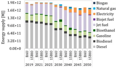
3.1 Dynamic inventory results 3.1.1 Partial‐equilibrium model biomass outputs and energy pathways Fig. 3 shows the primary biomass supply outputs [in Mt], from the PEM, of the BAU and 15Bio scenarios from 2019 to 2050, whereby Fig. 3a relates to energy mix + transport and Fig. 3b to the transport sub‐ sector. The biomass commodities described in the PEM were dedicated energy crops (corn, triticale, wheat, sugar beet, rapeseed, sunflower, palm oil, soybean), dedicated lignocellulosic material (LGC: miscanthus and other perennial crops), and residual biomass (FoWooR, from forestry and agriculture). The commodity category “energy crops” includes renewable resources associated with first generation (1G) biofuels, while dedicated LGC material and residual biomass associate with 2G biofuels. All described commodity were first exported from the PEM, as shown in Fig. 3a, to identify the pathways linked to transport end‐users. The commodity with the largest primary biomass share of the biomass supply was FoWooR, with proportions of up to 68% and 71% for BAU and 15Bio respectively. Annual mean values for FoWooR were estimated at 32 Mt for BAU and 34 Mt for 15Bio. The new set of policy constraints did not significantly change the FoWooR outputs over the PEM simulation TH, as compared with BAU. However, LGC material was introduced as a new commodity in the 15Bio scenario. Fig. 3. TIMES‐MIRET primary biomass supply from 2019 to 2050 per BAU and 15Bio scenarios of a) Energy mix (heat and electricity) and transport, and b) Transport sub‐sector only An in‐depth assessment of the transport sub‐sector pathways, demonstrated a shift of the biomass commodities from the energy mix + transport to the transport sub‐sector between BAU and 15Bio. FoWooR and agricultural residues, as well as LCG material, were mobilised for transport fuel processes, as shown in Fig. 3b. The LGC material commodity was introduced to feed the transport sub‐sector, as compared with all commodities in the energy mix + transport PEM outputs (Fig. 3b). A comparison among the scenarios, demonstrated that under BAU conditions, transport biofuels would exclusively be produced from energy‐crops. 1G biofuels would remain the only substitute to petroleum fuel. The other biomass commodity pathways in BAU would feed the energy mix (i.e. electricity heat cogeneration processes for other end‐users) only. In the 15Bio scenario, the mobilisation of FoWooR supply to transport was linked to the production of cellulosic bioethanol. It represented the only feedstock for 2G bioethanol. Peak 2G bioethanol production values were estimated in the year 2030, amounting up to 21 Mt (35% of the total biomass share for transport). Fig. 4 shows the final energy consumption share [in MJ] of the transport sub‐sector, per scenario, from 2019 to 2050. The depicted energy carriers represent the end‐user energy demand by a wide range of transport means. The prospective supply is based on the number of kilometres travelled per transport

(15)

means. It is expected that the final energy share will slightly decrease under the given assumptions, as more passengers would travel per trip of all transport means. The bioethanol energy carrier includes both 1G and 2G biofuels, whereas FoWooR represented the main feedstock for 2G cellulosic bioethanol production (in the 15Bio‐transport scenario). Other potential biofuel pathways and process outputs, such as Fisher‐Tropsch biodiesel, were not simulated under the new set of policies. In contrast, under BAU constraints, only 1G bioethanol from energy crops would be produced. Fig. 4. Final energy consumption in the transport sub‐sector per energy carrier and per scenario The new commodity and energy pathways in the transport sub‐sector were created in response to the new policy constraints (15Bio scenario). Compared with the BAU reference, the energy‐market dynamics changed in response to the policy constraint by optimising the outputs to secure energy supply by cost‐ effective means. These outputs are supposed to partially substitute 1G biofuels and petroleum fuels. Yet, the overall share of FoWooR, and thus that of 2G bioethanol to the transport sub‐sector, remained less significant than the share of energy crops for 1G biofuels, up to the year 2050. 3.1.2 Biogenic carbon balance from forest wood residues

Fig. 5 shows the Cbio balance results of FoWooR for the transport sub‐sector, under both BAU and 15Bio

scenarios, expressed in Mt Cbio. The Cbio flows for the BAU reference were zero, as no FoWooR were

accounted for the transport pathway (Fig. 5a). The flows from the historic Cbio fixation were inventoried as

negative (sequestration) and the Cbio combustion as positive (release back to the atmosphere). A full‐time

accounting with no temporal cut‐offs, allowed differentiating all Cbio flows of fixation and release through

time. The LCI TH was defined as the 1819 to 2050 period. The PEM simulation TH (2019 to 2050)

represented the years of final harvest (final fixation flow) and the years of production and consumption of FoWooR‐based 2G bioethanol (release flows). The first Cbio fixation flow started in the year 1819, due to the

application of a historic full‐rotation length of 200 years (see section 2.3.1). From the year 1819 onwards, the Cbio fixation values were accumulated until the final harvest in the year 2019. This has been repeated

for each following simulation year until 2050, which is the end year of the Cbio balance for both negative

(16)

Fig. 5. Dynamic biogenic carbon (Cbio) balance of residual forest wood biomass [Mt Cbio∙yr‐1] in the transport sub‐

sector with historic fixation (positive) and EOL combustion (negative) flows of a) BAU scenario, and b) 15Bio scenario

Under the assumption of combustion as EOL, the total Cbio fixation (‐1.01E8 Mt Cbio) and release (+1.01E8

Mt Cbio) flows sum up to zero, with no temporal cut‐offs. The area below the curve is equal for both flows,

meaning that the total Cbio embedded in the FoWooR is emitted back to the atmosphere during 2019 and

2050. This confirms that 100% of fixed Cbio is released back, as presumed under the carbon neutral

hypothesis. Yet, the annual biogenic values are not carbon neutral and, therefore, not zero. The time‐ explicit differentiation of the Cbio flows, describes the temporal Cbio emission profiles on an annual basis.

The sum of negative and positive Cbio values per year form the Cbio balance, representing the dynamic

biogenic inventories that can subsequently be assessed by means of the dynamic LCIA method. 3.1.3 Complete carbon flows of a specific year The dynamic inventories, both from fossil and biogenic sources, can be presented for a specific year of the modelled period. The calendar year representation is informative, as it details the flows and stocks of materials and energy on a key year of the policy‐based scenario. We selected the year 2030, a future key target‐year of the EU and national climate‐energy policy [110], generating top FoWooR supply estimates in the 15Bio scenario of the transport sub‐sector. All fossil and biogenic input and output flows were expressed in Mt C. Conversion factors from the EC‐JRC [81] were used to express all inventoried petroleum and biomass feedstocks as C. For the FoWooR commodity, we used the weighted mean of C content in wood (0.4952) from the Cbio model (Albers et al. in press). The elementary C flows from the feedstock

supply, transformation, use and EOL, were plotted in a Sankey‐style diagram, using the STAN v6.2 software [111]. The incoming C embedded in petroleum fuels and biofuels equals the outgoing C embedded in atmospheric emissions. Losses from biochemical or thermochemical processes in biofuel production pathways are presented here as wastes. The biofuel from residual lignocellulosic material yield of biochemical processes generates between 110 and 300 litres [26] of bioethanol per dry tonne of wood, with low heating values between 21.1 [26] and 26.8 MJ per litre [112]. The overall conversion efficiency of biochemical process pathway (likewise thermo‐chemical processes) is about 35%. The C flows (fossil + biogenic) of the transport sub‐sector under the BAU and 15Bio scenarios are shown in Fig. 6a and Fig. 6b, respectively. The biogenic flow (5.3 Mt C) shown in Fig. 6b corresponded to the Cbio balance of fixation + release dynamics at the year 2030. The total emitted Mt of C, including the biogenic flows, is higher for the 15Bio scenario by 4.5 Mt C. Without the biogenic flows, C outputs would be lower for 15Bio. For the specific calendar year 2030, the Cbio balance results revealed the highest value from

(17)

fixation and release, which then decreased to zero in the year 2050. The comparison among the scenarios showed that biogenic flows were only linked with the 15Bio for the transport sub‐sector. This questions whether the comparison with the BAU reference is valid. This issues is further addressed in section 3.3 with the introduction of a hypothetical BAU* scenario associated with a Cbio balance featuring an alternative EOL

pathway. Fig. 6. Carbon flows [Mt C] at year 2030, as Sankey‐type diagrams, from biogenic and fossil sources of the transport sub‐sector under a) BAU and b) 15Bio scenarios. Advanced second generation biofuels are not accounted for in the BAU scenario 3.2 Dynamic climate change impact results from the transport and bioethanol systems The dynamic impact assessment of the inventoried GHG emissions was performed with time‐dependent CFs [47], expressed as relative climate change impact in Mt CO2‐eq. The LCIA TH is variable in the dynamic method, and therefore an end year for the characterisation must be chosen by the practitioner to compare the results. We set the end year to 2119, 100‐years into the future from the first PEM simulation year (2019). The climate impact is computed per scenario as shown in Fig. 7, for both the transport sub‐sector (Fig. 7a) and the FoWooR‐based 2G bioethanol (Fig. 7b). The impacts per system and scenario were compared as per two sets of results, namely one based on C neutral estimates (without Cbio) and on

complete C estimates (with Cbio). Note that the BAU scenario revealed no climate change impact from Cbio,

since no Cbio balance (i.e. from 2G bioethanol) has been accounted in the reference simulations.

The climate change impact shown in Fig. 7a was based on all GHG emissions of the overall transport flows (i.e. production and consumption of petroleum fuels and biofuels). The climate change impact in 2119 would result in 1.19E3 and 1.11E3 Mt CO2‐eq, for BAU and 15Bio respectively. The new set of policies mitigate the climate change effects by 7% more, compared to BAU in the year 2119. The impacts remained under the BAU curve, even with projections beyond the selected chosen end year (not shown in Fig. 7a). Yet, fossil‐based results of both scenarios demonstrated a continuous increase of the atmospheric impacts. This is due to the annually accumulated impacts and the long‐term persistency of the dominant gas in the atmosphere (CO2). Even though CH4 and N2O have a higher perturbation capacity in the atmosphere, the

atmospheric residence lifetime (i.e. removal time in the atmosphere) of the reference CO2 gas is in the

order of thousands of years [43].

A comparison between the C neutral and the complete C results for transport, across scenarios (Fig. 7a), revealed that the climate change impact, and thus the mitigation effect from Cbio estimates from the BAU

reference scenario, are zero (as no FoWooR have been accounted for). Therefore, the comparison between C neutral and complete C was only valid for the 15Bio scenario. The 15Bio complete C impacts amount to 1.08E3 Mt CO2‐eq in the year 2019. Compared with the 15Bio C neutral impact (1.11E3 Mt CO2‐eq), it

(18)

higher mitigation effect than for 15Bio C neutral estimates. The reduction draws back to the inventoried historic long‐term sequestration period. This effect is sustained far into the future, until a steady‐state is achieved after about one thousand years (not shown in Fig. 7a). That is to say, in the distant future the complete C impacts become equivalent to the C neutral impacts.

Such a small estimated mitigation effect from the 15Bio complete C of the transport sub‐sector, is due to the dynamic Cbio balance corresponding exclusively to the FoWooR‐based 2G bioethanol pathway, which is

minimal compared with all fossil sourced emissions from the entire transport sector. The total 15Bio contributions of FoWooR to the transport sub‐sector, in the peak year 2030, amounted to 17% of the primary biomass share and 3% of the final energy consumption. The allocation of Cbio emissions to the

overall transport system were thus not significantly contributing in the 15Bio simulations. Therefore, an allocation of the Cbio emissions restricted to the FoWooR‐bioethanol pathway was undertaken to provide

insights into the climate change impact and mitigation effect of the bioethanol system.

Fig. 7. Relative climate change impact [Mt CO2‐eq], assessed by means of time‐dependent characterisation factors

based on the radiative forcing method for a) the transport sub‐sector, and b) the bioethanol systems

Results from the bioethanol system are shown in Fig. 7b. For the impact assessment of bioethanol, the following conversion factors were applied to the 15Bio FoWooR outputs: low heating value of 18.5 MJ∙kg‐1, bioethanol yield of 0.3428 MJEtanol∙MJwood‐1, and fossil‐based GHG emission factor of 19.5 g CO2‐eq∙MJEthanol‐1.

The CO2‐equivalent values were recalculated proportional to the respective CO2, CH4 and N2O elementary

flows given by the EC‐JRC [81] and divided by the default IPCC GWP100 equivalent factors [43]. The complete

C balance included the dynamic biogenic emissions from Cbio fixation and Cbio combustion EOL of FoWooR.

The C neutral estimates from bioethanol production were calculated using the EC‐JRC WTW method for EU farmed or waste wood‐to‐bioethanol pathways [81]. The cumulative bioethanol production from the FoWooR output associated with the 15Bio scenario over the entire PEM simulation TH amounted to 1.04E12 MJEthanol, which corresponds to a carbon footprint of 2.03E7 Mt CO2‐eq (when using the static

GWP100). A comparison between the absolute value of the total dynamic biogenic emissions from either Cbio fixation or combustion (3.72E2 Mt CO2‐eq) and the total fossil emissions from bioethanol production (2.03E7 Mt CO2‐eq), demonstrated that the fossil sourced emissions represented only about 5.4% of all emissions from the bioethanol system. Although the comparison is static ―all technical and elementary flows are summed up in the year 2019, equivalent to the year zero in static inventories―, the outcomes have shown the difference in orders of magnitude between the fossil and biogenic emissions in the bioethanol system. The relative climate change results from bioethanol (Fig. 7b) in the year 2119 resulted in 7.55E0 Mt CO2‐eq for C neutral and ‐2.74E1 Mt CO2‐eq for complete C. Note that for the BAU scenario has zero impact, as no

(19)

Cbio balance from FoWooR was accounted for and thus no production of bioethanol was modelled. A comparison between the two results for 15Bio Bioethanol showed that the climatic impacts for complete C are negative, implying that the sequestration is larger than the positive impact from the release. These complete C results would reduce those of C neutral results by 462%. Such high mitigation effect is explained by the low contribution (5.4%) of fossil sourced emissions to the total bioethanol emissions, and the duration of inventoried (historic) long‐term sequestration. Projections beyond the year 2119, revealed that the complete C results would continuously converge towards the C neutral curve. The climate mitigation effect is thus sensitive to a specific year or selected future reference year (i.e. end year of the LCIA impact assessment), as the LCIA TH is variable. Additionally, we calculated a dynamic emission factor for bioethanol from FoWooR. First, the relative climate impact for the Cbio balance (i.e. biogenic only) was computed the year 2119, resulting in ‐3.49E7 Mt

CO2‐eq. This negative value was subsequently divided by the total FoWooR‐bioethanol production (1.04E12

MJEthanol). The resulting dynamic emission factor (‐33.6 g CO2‐eq∙MJEthanol‐1) was contrasted with the EC‐JRC

static emission for wood residues from farmed forestry (19.5 g CO2‐eq∙MJEthanol‐1). A comparison between

these factors demonstrates that the dynamic factor is negative, which would imply that the climate impact from bioethanol production could be reduced by 272%, an almost three‐fold reduction for this specific policy scenario. This negative factor derives from the historic long‐term Cbio sequestration period assessed

in this study. However, the more distant into the future the reference year is set to, the lower the mitigation effect becomes, as the impact from biogenic sources approach C neutral results. That is to say, the negative atmospheric impact from sequestration is reduced thorough the positive impact from combustion. 3.3 Comparison of bioethanol impacts with an alternative reference scenario For the bioethanol system a comparison was undertaken between the 15Bio scenario and a hypothetical BAU* reference scenario featuring a Cbio balance with an alternative EOL pathway. This comparison was

performed because the previous BAU reference results were zero due to the absence of a Cbio balance

estimate. We therefore assumed a reference system, in which FoWooR from logging operations are left behind instead of being used for the transport sub‐sector. The hypothetical Cbio balance for the BAU*

scenario was composed from Cbio fixation and Cbio decay flows. It accounted for the same mass of FoWooR

described in the 15Bio scenario with the same historic full‐rotation length of 200 years (see section 2.3.1). Erreur ! Source du renvoi introuvable.a shows the Cbio balance from BAU* and 15Bio. The BAU* Cbio

fixation values were equal to those inventoried in the Cbio balance of the 15Bio scenario. The flows from the

EOL options however differed for combustion and decay. A comparison between the two inventoried EOL flows, indicated that the BAU* gradual decay of FoWooR shifted the release of emissions further into the future, as compared with the instant emissions from combustion. The last release flow from combustion occurred in the year 2050. For the decay, the last flow was estimated in the year 2119, although <0.01% of the carbon remained in the technosphere. We neglected those remaining emissions and assumed that until the year 2119 the total embedded carbon in the FoWooR returned to the atmosphere. Erreur ! Source du renvoi introuvable.b shows the relative climate change impact from the bioethanol system for BAU* and 15Bio. For bioethanol C neutral results (i.e. fossil based) are equal for both BAU* and 15Bio, amounting to 7.55E0 Mt CO2‐eq in the year 2119. The impact results of the complete C estimates would attain in Mt CO2‐eq 3.14E1 and ‐2.74E01 for BAU* and 15Bio respectively. The results for the BAU* with EOL decay are positive compared to those of 15Bio with combustion. This implies that the C neutral results from BAU*or 15Bio would be increased by 316%. This large difference compared to 15Bio derived

(20)

from the presence of short‐lived CH4, with high perturbation capacity, that was only considered in the EOL of BAU*. The CH4 decay emissions amounted to 10% of the total emissions associated with belowground biomass ratio, corresponding to the aboveground FoWooR, with a half‐life of 30 years. Fig. 8. a) Dynamic biogenic carbon [Cbio] balance of forest wood residues [Mt Cbio∙yr‐1] with fixation and two EOL options concerning combustion (15Bio scenario) and decay (BAU* alternative scenario), and b) relative climate change impact [Mt CO2‐eq] of the bioethanol system of both scenarios BAU* and 15Bio 3.4 Sensitivity analysis

To test the sensitivity of the Cbio model to the values of its key parameters, such as the growth rate, we

recalculated tree growth for all species with extreme initial values for all the parameters (from the acceptable range of values indicated in the literature). The acceptable range of values for the growth rate parameter k (growth rate) lied between 0.2 and 2.5. The CR model is rather robust and converges towards the originally computed results. The model is thus very flexible and accurate, yet it confirms its validity to the “slight expense of biological realism” [113].

Additionally, a sensitivity analysis was performed concerning the rotation length for the Cbio fixation of the

15Bio scenario. The previously applied 200‐year full rotation length was contrasted against 131 years, which is the weighted mean of rotation lengths of all tree species assessed in the Cbio fixation model. For

differentiation purposes, the scenario with the alternative full rotation length was named 15Bio*. Fig. 9 shows the sensitivity between the two rotation lengths for both systems under assessment, namely, the transport sub‐sector and the bioethanol. The dynamic climate change impact, as per the complete C balance, were compared for 15Bio and 15Bio*. The alternative rotation length generated a new LCI TH, as the first fixation year shifted from 1819 to 1888. The end year 2119 would generate the following climate change impact in Mt CO2‐eq: for the transport sub‐sector 1.08E3 (15Bio) and 1.36E3 (15Bio*), and for bioethanol ‐2.74E1 (15Bio) and 7.28E1 (15Bio*). The outcomes revealed high sensitivity for the rotation length of the Cbio fixation: the shorter the length the lower the mitigation effect (expressed as the