: Coupling Input-Output Tables with Macro-Life Cycle Assessment to Assess Worldwide Impacts of Biofuels Transport Policies

Titre:

Title

: Coupling Input-Output Tables with Macro-Life Cycle Assessment to Assess Worldwide Impacts of Biofuels Transport Policies

Auteurs:

Authors

: Audrey Somé, Thomas Dandres, Caroline Gaudreault, Guillaume Majeau-Bettez, Richard Wood et Réjean Samson

Date: 2017

Type:

Référence:

Citation

:

Somé, Audrey, Dandres, Thomas, Gaudreault, Caroline, Majeau-Bettez, Guillaume, Wood, Richard et Samson, Réjean (2017). Coupling Input-Output Tables with Macro-Life Cycle Assessment to Assess Worldwide Impacts of Biofuels Transport Policies. Journal of Industrial Ecology. doi:10.1111/jiec.12640

Document en libre accès dans PolyPublie

Open Access document in PolyPublie

URL de PolyPublie:

PolyPublie URL: http://publications.polymtl.ca/2645/

Version: Version finale avant publication / Accepted version Révisé par les pairs / Refereed

Conditions d’utilisation:

Terms of Use: CC BY-NC-ND

Document publié chez l’éditeur officiel

Titre de la revue:

Journal Title: Journal of Industrial Ecology Maison d’édition:

Publisher: Wiley & Yale University URL officiel:

Official URL: http://dx.doi.org/10.1111/jiec.12640

Mention légale:

Legal notice:

This is the peer reviewed version of the following article: Somé, A., Dandres, T., Gaudreault, C., Majeau-Bettez, G., Wood, R. and Samson, R. (2017), Coupling Input- Output Tables with Macro-Life Cycle Assessment to Assess Worldwide Impacts of Biofuels Transport Policies. Journal of Industrial Ecology. doi:10.1111/jiec.12640, which has been published in final form at http://dx.doi.org/10.1111/jiec.12640. This article may be used for non-commercial purposes in accordance with Wiley Terms and Conditions for Self-Archiving.

Ce fichier a été téléchargé à partir de PolyPublie, le dépôt institutionnel de Polytechnique Montréal

This file has been downloaded from PolyPublie, the institutional repository of Polytechnique Montréal

http://publications.polymtl.ca

Coupling I/O Tables with Macro-LCA to Assess Worldwide Impacts of Biofuels Transport Policies

Audrey Somé, Thomas Dandres, Caroline Gaudreault, Guillaume Majeau-Bettez, Richard Wood, Réjean Samson

Keywords: biofuel, land use, life cycle assessment (LCA), policy analysis, GTAP, EXIOBASE.

Abstract

Many countries see biofuels as a replacement to fossil fuels to mitigate climate change.

Nevertheless, some concerns remain about the overall benefits of biofuels policies. More comprehensive tools seem required to evaluate indirect effects of biofuel policies. This article proposes a method to evaluate large-scale biofuel policies that is based on life cycle assessment, environmental extensions of I/O tables and a general equilibrium model. The method enables the assessment of indirect environmental effects of biofuels policies including land use changes in the context of economic and demographic growths. The method is illustrated with a case study involving two scenarios. The first one describes the evolution of the world economy from 2006 to 2020 under business as usual (BAU) conditions (including demographic and dietary

preferences changes) and the second integrates biofuel policies in the USA and the European Union. Results show that the biofuel scenario, originally designed to mitigate climate change, results in more GHG emissions when compared to the BAU scenario. This is mainly due to emissions associated with global land use changes. The case study shows that the method enables a broader consideration for environmental effects of biofuel policies than usual LCA:

global economic variations calculated by a general equilibrium economic model and land use

change emissions can be evaluated. More work is needed however to include new biofuel

production technologies and reduce the uncertainty of the method.

Introduction

Life cycle assessment of biofuels

Over the past few years, with the rising levels of greenhouse gas (GHG) emissions and sustained concerns about climate change, biofuels have been seen as a promising solution to replace fossil fuels. Massive production of biofuels began in 2005 with a production of 53 billions liters of biofuels and rose over 138 billion globally in 2012 (OECD and FAO 2011).

Second generation biofuels (produced from cellulose) are developing fast, and third generation biofuels (from algae) are under active research (Scott et al. 2010), but neither of them can be industrially produced yet (Steynberg and Dry 2004a; Naik et al. 2010; Steynberg and Dry 2004b). Although first generation biofuels were often presented as an important part of climate change mitigation strategy as reviewed by Timilsina and Mevel (2013), there is still considerable uncertainty about their environmental benefits. Indeed, when the whole life cycle is evaluated, first generation biofuels are rarely climate neutral and the expected reductions in GHG emissions when compared to conventional fuels are fewer than expected or can even be higher than the emissions of conventional fuels (Benoist et al. 2012; Cherubini et al. 2009; Boies et al. 2011;

Kendall and Chang 2009; Menichetti and Otto 2009; Yang et al. 2012; Zah et al. 2007;

Soimakallio and Koponen 2011; Hsu et al. 2010; Halleux et al. 2008; Cherubini and Jungmeister

2010; Cherubini and Ulgiati 2010; Fazio and Monti 2011). One important methodological

concerns in the assessment of biofuels is the evaluation of direct and indirect land use changes

(LUC) since they are related to potentially significant carbon emissions to the atmosphere

(Panichelli and Gnansounou 2008; Mathews and Tan 2009; Plevin et al. 2010). Direct LUC

occur when a land is converted to grow biomass to produce bioenergy. Indirect LUC occur when

a land used for agriculture or forestry is converted to grow biomass for bioenergy production and

that the missing biomass for agriculture or forestry is grown on another land (the indirect LUC being the land displacement on the second land). While it may be simple to identify where direct LUC occur, indirect LUC causal links are more complex to model since they might consist in several sequential LUC affecting a lot of different crops and land types around the world.

Moreover, unlike direct LUC, indirect LUC cannot be physically monitored because they depend on land market evolution which is determined by a high numbers of parameters not restricted to the biomass demand for biofuels (Finkbeiner 2014; Wicke et al. 2012; Angus et al. 2009).

Nevertheless, the location and the quantity of land affected by indirect LUC are important parameters because carbon emissions from land conversions are strongly related to the types of land and the biomass affected by the LUC. Thus, the method used to model LUC emissions is highly uncertain and usually explain why results differ between biofuels studies (Kim and Dale 2011; Plevin et al. 2010; Finkbeiner 2014; Wicke et al. 2012; Malça and Freire 2011; Stratton et al. 2011).

Consideration of direct and indirect land use changes

Bird et al. (2013) consider two approaches to assess LUC: (1) the determinist approach which stands on simple mathematical relations based on historic data of the agriculture sector

(Overmars et al. 2011; Kim and Dale 2011; Wallington et al. 2012; Özdemir et al. 2009;

Silalertruksa et al. 2009; Escobar et al. 2014; Reinhard and Zah 2009) and (2) the economic approach which involves economic models to simulate the land market (United States Environmental Protection Agency 2009; Melillo et al. 2009a; Bird et al. 2013; Kendall and Chang 2009; Kloverpris 2009; Vázquez-Rowe et al. 2014; Sanchez et al. 2012; Verburg et al.

2008; Hertel et al. 2010; Hellmann and Verburg 2010; Britz and Hertel 2009; Keeney and Hertel

1 We also included LUC scenarios based on historic data in the determinist approach.

2008; Taheripour et al. 2010; Searchinger et al. 2008; Britz and Hertel 2011). The advantages of the determinist approach are to be very transparent, easy to follow and to stand on measurable indicators. The economic approach provides, however, a more refined understanding of the mechanisms that drive LUC, as economic phenomena and the land markets are explicitly modeled. While the numbers computed with both approaches may be quite different from one case study to another, a large majority of authors agree to say that GHG emissions related to direct and indirect land use changes are important and must be considered when evaluating biofuels ecological impact (Fritsche et al. 2010; Sanchez et al. 2012; Finkbeiner 2014).

One potentially important limit in existing biofuel studies is that these studies usually focus on a specific biofuel production assuming the rest of the world is not changing over the temporal horizon of the study. This approach is not consistent with methods that aim to include all land use drivers to study global prospective emissions scenarios (Vuuren et al. 2011b; Vuuren et al. 2011a).

In the case of the economic approach, it is known that equilibrium models provide non- linear responses to economic shocks. Thus, it might be an oversimplification to evaluate LUC caused by a single regional biofuel policy without including other parameters driving LUC at world scale: future biofuel demand in other regions, global food demand and dietary preferences (Haberl et al. 2011). Indeed, equilibrium models should lead to a different demand for land if all of these parameters are taken into account simultaneously, and thus lead to different LUC results and GHG emissions for biofuel policies.

Some authors recommend defining a baseline LUC scenario based on land market drivers

to conduct prospective studies on land use changes (Kloverpris and Mueller 2013; Westhoek et

al. 2006; Alcamo et al. 2006). No biofuel studies were found however to include all of the main

market drivers (i.e. global biofuel demand, global food demand and changes in dietary

preferences) along with a complete lifecycle perspective. Rather, these parameters are separately addressed in multiple individual studies, notably: Melillo et al. (2009b), Banse et al. (2011) and Bouët et al. (2010) consider both biofuel policies being implemented simultaneously in several regions and the future global food demand. Böttcher et al. (2013) include demography and food diet changes when assessing a European Union biofuel policy but they ignore other biofuel programs around the world. Thus, the objective of this research is to develop a method to study the environmental consequences of long-term biofuel policies being implemented simultaneously in the context of a growing food demand (due to the increasing world population) and a change in the global food-diet (increase in meat demand due to changes in dietary preferences in emerging countries).

Life cycle assessment and requirements for biofuel policies studies

Historically, most LCAs have taken a descriptive approach to product systems, striving to

account for the fraction of the environmental burdens that is physically linked to the production,

use, and end-of-life of a given product; this is often referred in the literature as attributional LCA

(A-LCA). In contrast, rather than assessing a product as a share of the economy, some LCAs

strive to capture the consequences of a perturbation to the economy, such as an increase in the

production for a given product. These models, which are collectively referred to as consequential

LCAs (C-LCA), attempt to follow relevant physical causation and market-mediated effects,

regardless of whether or not they are physically involved in the value chain of the product

(Weidema et al. 1999; Weidema 2003; Ekvall and Weidema 2004). Thus, compared to A-LCA,

C-LCA strives to directly model the consequences of a decision, such as a shift in consumption

or a policy, by analyzing the affected processes, regardless of whether they are inside or outside

of the product life cycle (Ekvall and Weidema 2004). Considering the land requirements for producing biofuels, an C-LCA approach is advantageous in order to model the market effects leading to indirect LUC, in contrast to A-LCA which only represents direct LUC. Several authors have pointed out that system boundaries and allocation rules related to biofuel co- products (defined in the goal and scope) were a source of significant heterogeneity in biofuel LCA results (Larson 2006; Cherubini et al. 2009; Davis et al. 2009; Cherubini and Strømman 2011; Benoist et al. 2012).

Additionally, since biofuel policies are planned over several years in the future, it is pertinent to follow a prospective LCA approach to take into account the temporal evolution of the studied system (Pesonen et al. 2000; Sanden 2007). Especially, in biofuel studies, the prospective approach should define the future biofuel targets to be studied and the evolution of the demographic and economic backgrounds during the period of implementation of the biofuel policies.

Environmental Input/Output LCA

Life cycle inventory (LCI) compiled using a process database are always truncated to a certain degree because it would not be practical to collect detailed data for all processes involved in the economy of a region (Suh and Huppes 2005). Thus, there is always a cut-off criteria in the inventory of process-based LCA. To solve that issue, environmental I/O databases were

introduced in LCA. Environmental I/O tables are a top-down environmental model of the entire

economy; they reflect the monetary interdependencies between all industries in the economy of a

region and the physical dependencies of these industries on the environment. In these databases,

each technological activity is related to an economic sector and emissions and natural resources

consumptions are obtained from national statistics of each economic sector (Suh 2003). Some

limitations are relying however solely on environmental I/O tables in LCA. Economic sectors in environmental I/O tables are often very aggregated (Egilmez et al. 2013). Thus, it is usually not possible to reach the same level of detail as when process databases are used to build the LCI.

Additionally, national I/O tables are country specific, which limits their ability to represent international production chains. For that reason, projects such as EXIOBASE (Tukker et al.

2014; Wood et al. 2014) or WIOD projects (Timmer 2012) compile multiregional, world environmental I/O tables.

Finally, I/O tables are based on historic data and fixed technological interdependencies.

As such, they are well suited for carbon footprinting and other attributional analyses (Hertwich and Peters 2009), but they are ill-suited to represent the mechanisms of an economy reacting to a perturbation, like the introduction of biofuels in transports. For that reason, technological

changes are difficult to study with I/O tables (Ferrão and Nhambiu 2009). To overcome that issue and answer prospective or consequential questions, I/O models are extended with linear programming optimizations (Strømman et al. 2009; Duchin 2005), dynamic time series (Pauliuk et al. 2015; Idenburg and Wilting 2000) , or price elasticities in the case of computable general equilibrium (CGE) models.

Macro-LCA

While in theory the consequential perspective is applicable to any type of change, most C-LCAs evaluate environmental effects of marginal perturbations affecting one or a few life cycles, allowing for simple, lean and transparent models (Dalgaard et al. 2008; Ekvall and Andrae 2006; Ekvall and Weidema 2004; Frees 2008; Gaudreault et al. 2010; Hamelin et al.

2011; Lesage et al. 2006; Mathiesen et al. 2007; Pehnt et al. 2008; Reinhard and Zah 2009;

Schmidt 2004, 2008; Schmidt and Weidema 2008; Thomassen et al. 2008; Weidema et al. 1999;

Eriksson et al. 2007). Unlike marginal perturbations, non-marginal perturbations are expected to affect many life cycles. Indeed, they are expected to affect the whole economy. Therefore, the economic modeling behind C-LCA needs to be adapted to handle non-marginal perturbations. In this context Dandres et al. (2011) proposed the macro-LCA (M-LCA): a new approach based on the sequential application of GTAP (Global Trade Analysis Project), a computable general equilibrium model (CGEM), and LCA to study shortterm effects of non-marginal perturbations;

the use of the CGEM allowing the considerations of price variations and non-linear effects on each economic sector including those that are indirectly affected by the perturbation. The use of LCA allowing the assessment of environmental impacts since GTAP provides very limited information regarding emissions to the environment. Long-term effects of non-marginal perturbations can be studied by introducing prospective elements in M-LCA (Dandres et al.

2012). The approach proposed by Dandres et al. (2011, 2012) computes the life cycle inventory (LCI) using GTAP results and the ecoinvent database (description provided in the supplementary material). Because the ecoinvent database does not cover all economic activities, some economic sectors were partially or not modeled in Dandres et al. (2011, 2012) increasing the LCI

truncation problem.

As mentioned previously, environmental Input/Output (I/O) databases can be used to overcome that issue. Since GTAP provides very few information about emissions to the environment but relies on national I/O tables, there is an opportunity to couple GTAP with the emission factors of each economic sector of the environmental extension of an I/O database to compute the LCI of all economic sectors in an M-LCA. Such coupling is a new contribution to the applications of GTAP and EXIOBASE.

Objective

The main objective of this article is to develop a new approach of M-LCA based on linking the environmental component of an I/O table with economic responses modeled through a CGE, allowing the modeling of the impact on the environmental inventory for every sector of the economy in every region. This development is presented in a case study evaluating the environmental impacts related to the implementation of major biofuel policies increasing the biofuel share of transportation by 2020 and implemented simultaneously in the USA and European Union (EU 27).

Methods

Overview of the LCA method and case study

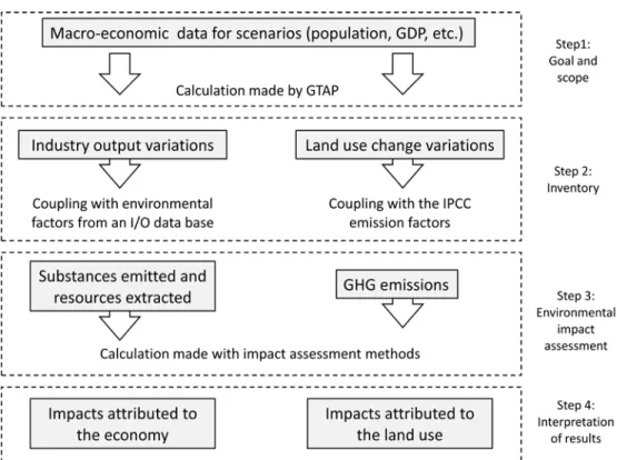
The method used in this study stands on the M-LCA developed in Dandres et al. (2012) and the steps of the method are summarized in Figure 1. The principle of the method relies on four sequential steps: to develop scenarios and implement them in GTAP (“goal and scope” step in Figure 1), to run GTAP simulations and map results with emission factors (“inventory” step in Figure 1), to apply impact assessment methods to compute environmental impacts (“impact assessment” step in Figure 1) and to analyze results (“results interpretation” step in Figure 1).

The method is divided into two parts (cf. left and right columns in Figure 1): the calculation of

the emissions triggered by a variation of activity in the economic sectors (obtained from coupling

GTAP with the environmental extension of an I/O Database) and the impacts of LUC (obtained

from coupling GTAP with IPCC factors).

Figure 1: LCA method used in the project.

Goal and scope definition

Two scenarios are compared to allow the distinction between the impacts caused by the

global economic growth (including demographic and dietary preference changes) from the

impacts due to the biofuel policies. The first scenario (referred later in the text as the reference

scenario) represents the evolution of the global economy from 2006 to 2020 under business as

usual conditions (with the exception that USA and EU 27 biofuel policies remain steady) and the

second one (referred as the biofuel scenario) integrates both the global economic growth and

more ambitious biofuel policies in the USA and the EU 27. The reference scenario integrates

exogenous drivers of expected changes in population, capital, gross domestic product (GDP),

skilled and unskilled workers and dietary preferences from 2006 (GTAP-BYP reference year) to

2020 (the desired year). The data are summarized in supplementary material (Table 3). In

addition to these drivers, the biofuel scenario incorporates the EU (European Commision 2012)

and the USA (U.S. Environmental Protection Agency 2012) estimated biofuels policies, based on existing regulations but adapted to focus only on first generation biofuels. Only first-generation biofuels are considered since the second generation of biofuels are currently not widely produced (therefore limited data are available to model it). Table 1 presents the share of biofuels in

transportation per region per year in the biofuel scenario (it is endogenously managed by GTAP- BYP for other economic sectors). The share of biofuels in the reference scenario in 2020 remains the same as in 2006. This reference scenario is, therefore, unlikely to happen since biofuel production is expected to increase in the future. The only purpose of the reference scenario in this study is to distinguish the specific environmental impacts due to the biofuel policies from those of the economic growth.

Region USA EU27

Year 2006 2011 2020 2006 2011 2020

Ethanol from cereal 3.13% 7.97% 9.31% 0.46% 0.98% 2.13%

Ethanol from sugar cane 0.07% 0.24% 2.05% 0.12% 0.24% 1.14%

Biodiesel from oilseeds 0.16% 0.62% 0.74% 1.1% 2.64% 6.7%

Table 1: Share of biofuels by volume in transportation by region for the biofuel scenario

GTAP-BYP includes only first generation biofuels. Since second and third generations of

biofuels are expected to have less environmental impacts than those of the first generation, the

results of this study might overestimate environmental impact if all biofuels would be considered

to reach targets of biofuel policies. Nevertheless, the work achieved in this study could be easily

adapted to a new version of GTAP-BYP that would include second and third generations of biofuels.

Inventory

The inventory is compiled using the environmental component of the I/O table of EXIOBASE (Tukker et al. 2013)

giving the unit of substance used/emitted per unit of

production of each economic sector based on the results of the GTAP-BYP simulations. The land use change factors from IPCC (Penman et al. 2003) are used to calculate GHG emissions from land use changes simulated by GTAP-BYP. More details regarding the application of the EXIOBASE table and GTAP model are presented in supplementary material.

Impact assessment

The impact assessment is done using the ReCiPe method (Goedkoop et al. 2013). The focus is made on GHG emissions but, based on the recommendations of Benoist et al. (2012) for biofuels, the eutrophication, acidification and ozone photochemical formation indicator are also included in the analysis.

GTAP

The economic model used in this M-LCA is GTAP-BYP, based on the GTAP model.

GTAP relies on national I/O tables to assess the variations due to a major change in the economy of a country, including non-linear effects (i.e. a response of the economy that is not proportional to the economic change). It calculates an optimal solution which enables equilibrium between supply and demand under specific constraints specified by the user. More details on GTAP-BYP are provided in supplementary material.

EXIOBASE

In order to study the global environmental impacts of biofuel policies with an

environmental I/O table, this table must be multi-region since consequences of biofuel policies might occur outside of the regions where the policies are implemented. EXIOBASE and WIOD are two currently available multi-regional I/O databases that would be fit for purpose.

EXIOBASE is preferred however since it allows to cover more environmental indicators and presents a finer granularity in its description of the agricultural sectors (Tukker and

Dietzenbacher 2013). In its most disaggregated version, the first version of EXIOBASE includes 43 countries and one region (Rest of World) and have data on 28 emission types to air (both combustion and non-combustion), as well as nitrogen and phosphorous emissions and use of resources for every economic sector (Tukker et al. 2013). The coupling of GTAP with EXIOBASE, as well as the modifications made on EXIOBASE are explained in the supplementary material.

Land use data

GTAP-BYP provides information about the area and type of land that are transformed (Lee et al. 2005). GTAP-BYP models four activities (sugar, cereal and oil crops; other crops;

pasture; and forests) spread into 18 agro-ecological zones that depend on the annual length of

growing period as well as the humidity conditions. IPCC proposed generic emission factors that

can be used to model GHG emissions from LUC (Penman et al. 2003). These emission factors

depend on several land characteristics such as the type of land (forest, crops or pasture),

geographical locations (boreal, tropical and temperate), and rain conditions (wet, dry). In this

study, IPCC factors were mapped with GTAP-BYP land types to compute LUC emissions. The

mapping is detailed in supplementary material.

While GTAP-BYP computes the total LUC for the period 2006-2020, the annual LUC emissions are obtained by dividing the total LUC emissions obtained from Equation 7

(supplementary material) by 14 years (the number of years of the scenarios).

Results and discussion

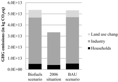
In this section, the global environmental impacts are presented first, then the impacts attributed to the industry, households and land use changes are analyzed, and then the difference between the scenarios and the limits of the method are discussed. Table 2 summarizes the GHG emissions per scenario, per region (USA, EU, and rest of world) and per category (industry, households and land use change) in 2020. It also presents the difference in GHG emissions between the biofuels scenario and the reference scenario. A negative result in the difference indicates a better performance of the biofuel scenario whereas a positive result indicates a better performance of the reference scenario.

GHG emissions per scenario

(Gt CO2eq/Functional unit) USA EU 27 REST OF

WORLD TOTAL

Biofuels 8.5 5.2 28.3 42.0

Industrial

production Reference 8.1 5.7 28.3 42.1

Difference* 0.3 -0.5 0.1 -0.1

Biofuels 1.1 0.1 3.8 5.0

Private household

consumption Reference 1.2 0.2 3.9 5.3

Difference* -0.1 -0.1 0.0 -0.3

Biofuels 0.6 0.4 5.8 6.8

Land use

change Reference 0.4 0.3 5.5 6.1

Difference* 0.3 0.1 0.2 0.6

Biofuels 10.2 5.7 37.9 53.8

Total Reference 9.7 6.1 37.7 53.5

Difference* 0.5 -0.5 0.3 0.3

*Values do not equal exactly to Biofuels minus Reference values due to hidden decimals.

Table 2: GHG emissions from industries, private households and land use in both scenarios It can be seen the industrial production is the main global emitter of GHG emissions, then come the land use changes and the private household consumption with smaller contributions. As expected, the land use change emissions are more important in the biofuel scenario than in the reference one. The main difference in GHG emissions between the scenarios is due to the land use change. These emissions are so significant in the biofuels scenario that they overcome the benefits of the biofuels policies observed in industrial production and private household consumption. Consequently, at the global level, the biofuels scenario is found to result in more GHG emissions than the reference scenario. This is consistent with other studies published in the literature (e.g., Searchinger et al. 2008; Hertel et al. 2009; Keeney and Hertel 2008; Plevin et al.

2010; United States Environmental Protection Agency 2009). It should be noted however the differences in GHG emissions between the two scenarios is relatively small when compared to the total GHG emissions of each scenario. These results are discussed in greater detailed for each category in the following paragraphs.

Industrial production emissions

The differences in environmental indicators results between the biofuel and reference

scenarios are depicted in Figure 2. A negative difference indicates that the biofuel scenario

would cause less impact than the reference scenario. On the contrary, a positive difference points

out that the biofuel scenario would be potentially more damaging than the reference one. It can

be seen the environmental indicators are not all affected in the same way. While the climate change tends to be less affected by the industrial production in the biofuels scenario, the

reference scenario performs better for the three other environmental indicators. This is consistent with what can be found in the literature (Benoist et al. 2012). Additionally, the contribution from the industrial production of each region to the environmental indicators is not the same. While the EU industrial production contributes the most to the climate change indicator, it contributes the less to the other indicators. Also, the acidification indicator is mainly affected by the USA industrial production while the eutrophication is mainly affected by the rest of world industry.

Globally, the contribution from the industrial production in the rest of the world for three of the four environmental indicators is relatively important (more than 60% in the case of

eutrophication). This result highlights the need for an approach enabling the capture of global

impacts of biofuel policies. Despite the implementation of biofuel policies in both the EU and the

USA, a large difference can be observed between these regions for all indicators.

Figure 2: Difference in environmental indicator results of industrial production between the biofuel and reference scenarios.

When looking at the rest of world region, it appears that Brazil is strongly affected by the policies: even though this country has not implemented a greater biofuel policy in the biofuels scenario, it appears to have more environmental impacts in the case of the biofuels scenario. This rise is due to the growing production of bioethanol from sugarcane in Brazil to meet the

requirement of the USA policy. Indeed in GTAP-BYP, the biofuel demand can be specified for each country, but the model allows global producers to fulfill this demand. That is the reason why there are Brazilian exportats towards the USA and so that Brazil is impacted by biofuel policies. This result is in accordance with Luo et al. (2009).

By capturing the evolution of the industry (through the changes of each economic sector), GTAP-BYP enables a broader view of the perturbation triggered by the biofuel policies than if

Eutrophication

(Mt Peq) Acidification (Mt SO2eq)

Photochemical O3 formation (Mt NMVOC)

Climate change (Gt CO2eq)

USA 0.06 3.15 0.08 0.34

EU 0.05 0.17 0.01 -0.47

Rest of World 0.18 1.00 0.08 0.06

-60%

-40%

-20%

0%

20%

40%

60%

80%

100%

USA EU

Rest of World

EXIOBASE would have been used without this economic model. Indeed, in this latter case, the results would not have been based on the evolution of the industry since inter industries

relationships would have remained unchanged, at the situation of 2000 (reference year of EXIOBASE version 1).

Private household emissions

GHG emissions for private households, presented above in Table 2, show that the biofuels scenario has less potential impacts than the reference scenario for each region. The impacts from the EU 27 are about one order of magnitude below the impacts of the USA, mainly due to the private consumption growth that is more important for the USA. It is also observed that differential GHG emissions from world private households are approximately three and a half times more important than differential emissions from world industries when the biofuel scenario and reference scenario are compared. This result confirms the modification of EXIOBASE regarding private household consumption emissions (presented in the supplementary material) is pertinent.

Land use change emissions

The differences between biofuels and references scenarios of annual land use change

GHG emissions per type of use and per region are presented in Figure 3. It shows that the biofuel

scenario causes globally more LUC emissions than the reference scenario. As expected, sugar,

oilseed and coarse grain crops that are required for the production of biofuels are more strongly

affected (causing more GHG emissions) in the US and EU in the biofuel than in the reference

scenario. Moreover, according to GTAP-BYP, important differences in LUC GHG emissions

between scenarios are related to pasture and forestry sectors. Indeed, regarding LUC, it is found

the biofuel scenario results in far more GHG emissions than the reference scenario for the pasture sector but in far less emissions for the forestry sector. For both of these sectors, GTAP- BYP anticipates most of the LUC emissions occur outside of the US and EU. This result highlights again the need to study LUC phenomena at world scale and not to restrict it to countries implementing biofuel policies.

Figure 3: Difference in GHG emissions from land use change of biofuel and reference scenarios.

When looking at the regional results, it can be noted that both the USA and EU 27 have more GHG emissions regarding the biofuel scenario than the reference scenario. More

specifically, the emissions from cereal, sugar, and oil crops are more important in the case of biofuel scenario for these two regions. The difference between USA and EU 27 that can be observed for cereal, sugar and oil crops, is due to the higher amount of land that is transformed to meet the requirements of the biofuels policy in the USA. These impacts do not represent

however the total share of world impacts regarding land use. This comes from the fact that both USA and Europe have agro-ecological zones that are very convenient for agriculture. Indeed, their agriculture zones are situated in temperate climate zone explaining why they are not as

-1.0E+00 -5.0E-01 0.0E+00 5.0E-01 1.0E+00 1.5E+00 2.0E+00

Ceral, sugar and oil

crops

Other

crops Pasture Forest All activities

LU C GH G e m iss io ns (Gt C O

eq )

Type of activity

World USA EU

affected as other countries in which climate is more challenging for crops (and so more important environmental factors).

These results also show that possible impacts have to be considered globally since the results can be positive in a region and negative in another. For instance, in Brazil, the results of biofuel policies are clearly negative (more GHG emissions). Indeed this country, according to GTAP-BYP, has to transform as much land as the USA to meet the sugarcane ethanol

requirements, a situation that triggers serious environmental effects.

As compared to the differences in GHG emissions from the industry and households categories between the biofuel and the references scenarios, the difference in LUC emissions are dramatically higher and therefore are determinant in the comparison of the scenarios (see Figure 4). Thus, when not considering land use change, the biofuels scenario performs better than the reference scenario but the opposite conclusion is obtained when considering LUC emissions.

This shows the importance of not neglecting LUC in biofuel studies.

Figure 4: Difference in GHG emissions between the biofuels and reference scenarios by region.

-0.8 -0.6 -0.4 -0.2 0.0 0.2 0.4 0.6 0.8

USA EU 27 Rest of

World Overall difference G H G em issi on s ( G t C O

eq)

Regions

Land use change

Industrial production

Private household

consumption

A more detailed analysis of the results obtained in EXIOBASE and GTAP provides the following insights. The inventory given by the I/O database shows that most impacted sectors for both scenarios are the energy intensive industries (such as the manufacture of chemicals or metals) and the other industries and services (such as transports). An analysis in the GTAP model has shown that the main contributor to these economic sectors (and as a matter of fact to these impacts) is both domestic sales as well as importations as opposed to exportations. When looking at importations and exportations between countries and by commodities, it is interesting to point out that the exchanges between countries are relatively constant when comparing the two scenarios. The differential impacts between the two scenarios are more related to the supply price. The supply price of commodities tends to rise among some specific commodities in the case of the biofuel scenarios, especially the agricultural products (e.g., paddy rice or cereals), as expected. A slight decrease from the commodities in energy intensive industries and in other industries and services can be observed, explaining the better environmental performance of the biofuel scenario when land use change is excluded. Indeed, even if the price and production of agricultural goods rise in the biofuel scenario, the impacts are not important enough to

counterbalance the decrease due to energy intensive industries. Thus, the coupling between the equilibrium model and the I/O database seems all the more pertinent when it comes to consider the economic reasons that are directly linked to the environmental impacts.

Total and differential emissions of the biofuels and reference scenarios

The method followed in this study enables to distinguish between the impacts of the economic growth (including demographic and dietary changes) and from the biofuel policies. It is shown the reference scenario is better than the biofuels scenario regarding the GHG emissions.

It is also pertinent however to compare the results of the scenarios to the initial situation (the

year 2006) in order to evaluate the trend of the global GHG emissions from 2006 to 2020.

Figures 5 put the overall GHG emissions of each scenario in the context of the economic growth over 2006-2020. A first observation is that the GHG emissions are significantly increased in both scenarios as compared to 2006. By comparing the contribution of each GHG emissions category it makes it possible to allocate GHG emissions to the biofuels policy or to the economic growth.

Thus, the economic growth is responsible for 94% of the change in GHG emissions over 2006- 2020 while the remaining 6% can be allocated to the effects of the biofuels policy. This means the biofuels policies have low influence on the future GHG emissions. This result is in

accordance with previous studies by Yang et al (2012) and by Dandres et al. (2012).

The largest contribution of GHG emissions from the economic growth comes from the industry while the contribution from land use change is still significant. When looking at the regional contributions of the land use change GHG emissions, it appears that most of these emissions come from the rest of the world (more than five times larger than from the USA and EU regions). Considering the rest of world region is more affected by the dietary change (see Table 3 in the supplementary material) than the USA and EU regions, this suggests the increased demand for meat in emerging countries is expected to have a large contribution to future GHG emissions. Nevertheless, the increase in population and resulting food demand are also

responsible for land use change GHG emissions.

Figure 5: Annual changes in GHG emissions in 2006 and in the biofuels and reference scenarios per category.

Limitations and uncertainty

In this study, it was shown that coupling GTAP-BYP with EXIOBASE makes it possible to assess several biofuel policies being implemented simultaneously in several regions in the context of evolving background. Moreover, it improves the results of policy assessment by both GTAP-BYP and EXIOBASE. Indeed, GTAP-BYP models changes in the economy (including demography, LUC, and dietary preferences) and EXIOBASE provide emissions factors to compute several types of environmental impacts from GTAP-BYP results instead of being restricted to GHG emissions. Nevertheless, some limitations are inherent to the choice of GTAP- BYP and EXIOBASE as well as the method to compute emissions from LUC: a limited number of substances in EXIOBASE, the fixed emission factors over the studied period, the fact that natural ecosystems are not convertible in land in GTAP-BYP, and the imperfect coupling of GTAP-BYP with EXIOBASE. These limitations are discussed in the supplementary material.

0.0E+00 1.0E+13 2.0E+13 3.0E+13 4.0E+13 5.0E+13 6.0E+13

Biofuels

scenario 2006

situation BAU scenario G H G em issi on s ( in k g C O

eq)

Land use change Industry

Households

Conclusions

The case study presented in this article suggests that the biofuel policies studied do not mitigate environmental impacts of climate change, eutrophication, ozone photochemical formation, and acidification when compared to business as usual conditions, especially when land use change impacts are considered. When compared to the expected economic growth (including demographic and dietary preference changes) in the timeframe considered, the difference between the two scenarios is however not very significant. The inclusion of the emissions due to land use change in the global impacts appears critically important in the evaluation of the biofuels scenario. It enables the consideration of more indirect impacts and greatly improves the completeness of this method. Especially, it reveals that regional biofuel policies are expected to cause emissions outside of the regions where they are implemented.

Nevertheless, some improvement needs to be achieved in order to give more precise results, especially given the uncertainty in data and models.

Using a general equilibrium model to calculate economic data that are then coupled

directly with environmental I/O tables is particularly relevant in the case of large-scale systems

since it enables a more complete life cycle assessment. Indeed, compared to the life cycle

assessments that determines the impacts of some processes or that focused on only a few

economic sectors, this method is able to provide environmental impacts across the whole

economy. Regarding the M-LCA developed by Dandres et al. (2011, 2012) and based on

ecoinvent, the macro-LCA based on EXIOBASE presented in this article is a new development

of the M-LCA method. It makes it possible to include all economic sectors but considers fewer

substances emitted or extracted from nature in the environmental impact assessment. The further

inclusion of missing substances in I/O databases would facilitate further coupling efforts.

Acknowledgments

The authors acknowledge the industrial partners of the International Chair in Life Cycle Assessment (a research unit of CIRAIG [Interuniversity Research Centre for the Life Cycle of Products, Processes and Services]) for their financial support: Alcan, Arcelor-Mittal, Bell Canada, Cascades, Eco-Entreprises-Québec/Recyc-Québec, Groupe EDF/GDF-SUEZ, Hydro- Québec, Johnson & Johnson, Mouvement des Caisses Desjardins, RONA, Total and Veolia Environnement.

References

Alcamo, J., K. Kok, G. Busch, J. Priess, B. Eickhout, M. Rounsevell, D. Rothman, and M.

Heistermann. 2006. Searching for the Future of Land: Scenarios from the Local to Global Scale. In Land-Use and Land-Cover Change, edited by E. Lambin and H. Geist:

Springer, Berlin, Heidelberg.

Angus, A., P. J. Burgess, J. Morris, and J. Lingard. 2009. Agriculture and land use: Demand for and supply of agricultural commodities, characteristics of the farming and food

industries, and implications for land use in the UK. Land Use Policy 26(Supplement 1):

S230-S242.

Banse, M., A. Tabeau, H. v. Meijl, G. Woltjer, and A. G. Prins. 2011. Global impact of multinational biofuel mandates on land use, feedstock prices, international trade and greenhouse gas emissions. In 14 th Annual Conference on Global Economic Analysis.

Venice, Italy.

Benoist, A., D. Dron, and A. Zoughaib. 2012. Origins of the debate on the life-cycle greenhouse gas emissions and energy consumption of first-generation biofuels - A sensitivity analysis approach. Biomass and Bioenergy 40(0): 133-142.

Bird, D. N., G. Zanchi, and N. Pena. 2013. A method for estimating the indirect land use change from bioenergy activities based on the supply and demand of agricultural-based energy.

Biomass and Bioenergy 59(0): 3-15.

Boies, A. M., D. McFarlane, S. Taff, W. F. Watts, and D. B. Kittelson. 2011. Implications of local lifecycle analyses and low carbon fuel standard design on gasohol transportation fuels. Energy Policy 39(11): 7191-7201.

Böttcher, H., S. Frank, P. Havlík, and B. Elbersen. 2013. Future GHG emissions more efficiently controlled by land-use policies than by bioenergy sustainability criteria. Biofuels,

Bioproducts and Biorefining 7(2): 115-125.

Bouët, A., B. V. Dimaranan, and H. Valin. 2010. Modeling the global trade and environmental

impacts of biofuel policies. Washington, D.C., USA: International Food Policy Research

Institute (IFPRI).

Britz, W. and T. W. Hertel. 2009. Impacts of EU biofuels directives on global markets and EU environmental quality: An integrated PE, global CGE analysis. Agriculture, Ecosystems

& Environment In Press, Corrected Proof.

Britz, W. and T. W. Hertel. 2011. Impacts of EU biofuels directives on global markets and EU environmental quality: An integrated PE, global CGE analysis. Agriculture, Ecosystems

& Environment 142(1–2): 102-109.

Cherubini, F. and G. Jungmeister. 2010. LCA of a biorefinery concept producing bioethanol, bioenergy, and chemicals from switchgrass. The International Journal of Life Cycle Assessment 15(1): 53-66.

Cherubini, F. and S. Ulgiati. 2010. Crop residues as raw materials for biorefinery systems - A LCA case study. Applied Energy 87(1): 47-57.

Cherubini, F. and A. H. Strømman. 2011. Life cycle assessment of bioenergy systems: State of the art and future challenges. Bioresource Technology 102(2): 437-451.

Cherubini, F., D. N. Bird, A. Cowie, G. Jungmeister, B. Schlamadinger, and S. Woess-Gallasch.

2009. Energy- and greenhouse gas-based LCA of biofuel and bioenergy systems: Key issues, ranges and recommendations. Resources, Conservation and Recycling 53(8): 434- 447.

Dalgaard, R., J. H. Schmidt, N. Halberg, P. Christensen, M. Thrane, and W. A. Pengue. 2008.

LCA of soybean meal. International Journal of Life Cycle Assessment 13(3): 1-15.

Dandres, T., C. Gaudreault, P. Tirado-Seco, and R. Samson. 2011. Assessing non-marginal variations with consequential LCA: Application to European energy sector. Renewable and Sustainable Energy Reviews 15(6): 3121-3132.

Dandres, T., C. Gaudreault, P. Tirado-Seco, and R. Samson. 2012. Macroanalysis of the

economic and environmental impacts of a 2005-2025 European Union bioenergy policy using the GTAP model and life cycle assessment. Renewable and Sustainable Energy Reviews 16(2): 1180-1192.

Davis, S. C., K. J. Anderson-Teixeira, and E. H. DeLucia. 2009. Life-cycle analysis and the ecology of biofuels. Trends in Plant Science 14(3): 140-146.

Duchin, F. 2005. A world trade model based on comparative advantage with m regions, n goods, and k factors. Economic Systems Research 17(2): 141-162.

Egilmez, G., M. Kucukvar, and O. Tatari. 2013. Sustainability assessment of U.S. manufacturing sectors: An economic input output-based frontier approach. Journal of Cleaner

Production 53: 91-102.

Ekvall, T. and B. P. Weidema. 2004. System boundaries and input data in consequential life cycle inventory analysis. International Journal of Life Cycle Assessment 9(3): 161-171.

Ekvall, T. and A. S. G. Andrae. 2006. Attributional and consequential environmental assessment of the shift to lead-free solders. International Journal of Life Cycle Assessment 11(5):

344-353

Eriksson, O., G. Finnveden, T. Ekvall, and A. E. Bjorklund. 2007. Life cycle assessment of fuels for district heating: a comparison of waste incineration, biomass- and natural gas

combustion. Energy Policy 35: 1346-1362.

Escobar, N., J. Ribal, G. Clemente, and N. Sanjuán. 2014. Consequential LCA of two alternative

systems for biodiesel consumption in Spain, considering uncertainty. Journal of Cleaner

Production 79(0): 61-73.

European Commision. 2012. Les objectifs d' Europe 2020.

http://ec.europa.eu/europe2020/europe-2020-in-a-nutshell/targets/index_fr.htm. Accessed 29/10 2013.

Fazio, S. and A. Monti. 2011. Life cycle assessment of different bioenergy production systems including perennial and annual crops. Biomass and Bioenergy 35(12): 4868-4878.

Ferrão, P. and J. Nhambiu. 2009. A Comparison Between Conventional LCA and Hybrid EIO- LCA: Analyzing Crystal Giftware Contribution to Global Warming Potential. In

Handbook of Input-Output Economics in Industrial Ecology, edited by S. Suh. Dordrecht:

Springer, Netherlands.

Finkbeiner, M. 2014. Indirect land use change – Help beyond the hype? Biomass and Bioenergy 62(0): 218-221.

Frees, N. 2008. Crediting aluminium recycling in LCA by demand or by disposal. International Journal of Life Cycle Assessment 13(3): 212-218.

Fritsche, U. R., R. E. H. Sims, and A. Monti. 2010. Direct and indirect land-use competition issues for energy crops and their sustainable production – an overview. Biofuels, Bioproducts and Biorefining 4(6): 692-704.

Gaudreault, C., R. Samson, and P. Stuart. 2010. Energy decision making in a pulp and paper mill: selection of LCA system boundary. International Journal of Life Cycle Assessment 15(2): 198-211.

Goedkoop, M. J., R. Heijungs, M. A. Huijbregts, A. D. Schryver, J. Struijs, and R. Van Zelm.

2013. A life cycle impact assessment method which comprises harmonised category indicators at the midpoint and the endpoint level. The Hague, Netherlands: Ministry of Housing, Spatial Planning and the Environment.

Haberl, H., K.-H. Erb, F. Krausmann, A. Bondeau, C. Lauk, C. Müller, C. Plutzar, and J. K.

Steinberger. 2011. Global bioenergy potentials from agricultural land in 2050: Sensitivity to climate change, diets and yields. Biomass and Bioenergy 35(12): 4753-4769.

Halleux, H., S. Lassaux, R. Renzoni, and A. Germain. 2008. Comparative life cycle assessment of two biofuels: ethanol from sugar beet and rapeseed methyl ester. International Journal of Life Cycle Assessment 13(3): 184-190.

Hamelin, L., M. S. Wesnaes, H. Wenzel, and B. M. Petersen. 2011. Environmental

Consequences of Future Biogas Technologies Based on Separated Slurry. Environmental Science & Technology 45(13): 5869-5877.

Hellmann, F. and P. H. Verburg. 2010. Impact assessment of the European biofuel directive on land use and biodiversity. Journal of Environmental Management 91(6): 1389-1396.

Hertel, T. W., A. A. Golub, A. D. Jones, M. O'Hare, R. J. Plevin, and D. M. Kammen. 2009.

Global Land Use and Greenhouse Gas Emissions Impacts of U.S. Maize Ethanol: The Role of Market-Mediated Responses. GTAP Working Paper No. 55. West Lafayette, IN, USA: Center for Global Trade Analysis, Department of Agricultural Economics, Purdue University.

Hertel, T. W., A. A. Golub, A. D. Jones, M. O'Hare, R. J. Plevin, and D. M. Kammen. 2010.

Effects of US Maize Ethanol on Global Land Use and Greenhouse Gas Emissions:

Estimating Market-mediated Responses. BioScience 60(3): 223-231.

Hertwich, E. G. and G. P. Peters. 2009. Carbon Footprint of Nations: A Global, Trade-Linked

Analysis. Environmental Science & Technology 43(16): 6414-6420.

Hsu, D. D., D. Inman, G. A. Heath, E. J. Wolfrum, M. K. Mann, and A. Aden. 2010. Life Cycle Environmental Impacts of Selected U.S. Ethanol Production and Use Pathways in 2022.

Environmental Science & Technology 44(13): 5289-5297.

Idenburg, A. and H. Wilting. 2000. DIMITRI: A dynamic input-output model to study the impacts of technology related innovations. In XIII International Conference on Input- Output Techniques. University of Macerata, Italy.

Keeney, R. and T. W. Hertel. 2008. The Indirect Land Use Impacts of U.S. Biofuel Policies: The Importance of Acreage, Yield, and Bilateral Trade Responses. Center for Global Trade Analysis, Department of Agricultural Economics, Purdue University.

Kendall, A. and B. Chang. 2009. Estimating life cycle greenhouse gas emissions from corn- ethanol: a critical review of current U.S. practices. Journal of Cleaner Production 17(13):

1175-1182.

Kim, S. and B. E. Dale. 2011. Indirect land use change for biofuels: Testing predictions and improving analytical methodologies. Biomass and Bioenergy 35(7): 3235-3240.

Kloverpris, J. H. 2009. Identification of biomes affected by marginal expansion of agricultural land use induced by increased crop consumption. Journal of Cleaner Production 17(4):

463-470.

Kloverpris, J. H. and S. Mueller. 2013. Baseline time accounting: Considering global land use dynamics when estimating the climate impact of indirect land use change caused by biofuels. The International Journal of Life Cycle Assessment 18(2): 319-330.

Larson, E. D. 2006. A review of life-cycle analysis studies on liquid biofuel systems for the transport sector. Energy for Sustainable Development 10(2): 109-126.

Lee, H.-L., T. W. Hertel, B. Sohngen, and N. Ramankutty. 2005. Towards An Integrated Land Use Data Base for Assessing the Potential for Greenhouse Gas Mitigation. West Lafayette (IN), USA: Purdue University, Global Trade Analysis Project (GTAP).

Lesage, P., T. Ekvall, L. Deschenes, and R. Samson. 2006. Environmental assessment of brownfield rehabilitation using two different life cycle inventory models. Part 2: case study. International Journal of Life Cycle Assessment 12(7): 497-513.

Luo, L., E. van der Voet, and G. Huppes. 2009. Life cycle assessment and life cycle costing of bioethanol from sugarcane in Brazil. Renewable and Sustainable Energy Reviews 13(6–

7): 1613-1619.

Malça, J. and F. Freire. 2011. Life-cycle studies of biodiesel in Europe: A review addressing the variability of results and modeling issues. Renewable and Sustainable Energy Reviews 15(1): 338-351.

Mathews, J. A. and H. Tan. 2009. Biofuels and indirect land use change effects: the debate continues. Biofuels, Bioproducts and Biorefining 3(3): 305-317.

Mathiesen, B. V., M. Munster, and T. Fruergaard. 2007. Energy system analyses of the marginal energy technology in life cycle assessments. Paper presented at SETAC Europe 14th LCA Case Studies Symposium, December 3-4, 2007, Goteborg, Sweden.

Melillo, J. M., J. M. Reilly, D. W. Kicklighter, A. C. Gurgel, T. W. Cronin, S. Paltsev, B. S.

Felzer, X. Wang, A. P. Sokolov, and C. A. Schlosser. 2009a. Indirect Emissions from Biofuels: How Important? Science 326(5958): 1397-1399.

Melillo, J. M., A. C. Gurgel, D. W. Kicklighter, J. M. Reilly, T. W. Cronin, B. S. Felzer, S.

Paltsev, C. A. Schlosser, A. P. Sokolov, and X. Wang. 2009b. Unintended Environmental Consequences of a Global Biofuels Program. Report no. 168. Cambridge, MA, USA:

Massachusetts Institute of Technology (MIT).

Menichetti, E. and M. Otto. 2009. Energy Balance & Greenhouse Gas Emissions of Biofuels from a Life Cycle Perspective. In Biofuels: Environmental Consequences and

Interactions with Changing Land Use, edited by R. W. H. a. S. Bringezu. Gummersbach, Germany: Cornell University.

Naik, S. N., V. V. Goud, P. K. Rout, and A. K. Dalai. 2010. Production of first and second generation biofuels: A comprehensive review. Renewable and Sustainable Energy Reviews 14(2): 578-597.

OECD and FAO. 2011. OECD FAO agricultural outlook 2011-2020. chapter 3: biofuels, edited by O. p. a. FAO.

Overmars, K. P., E. Stehfest, J. P. M. Ros, and A. G. Prins. 2011. Indirect land use change emissions related to EU biofuel consumption: an analysis based on historical data.

Environmental Science & Policy 14(3): 248-257.

Özdemir, E. D., M. Härdtlein, and L. Eltrop. 2009. Land substitution effects of biofuel side products and implications on the land area requirement for EU 2020 biofuel targets.

Energy Policy 37(8): 2986-2996.

Panichelli, L. and E. Gnansounou. 2008. Estimating greenhouse gas emissions from indirect land-use change in biofuels production: concepts and exploratory analysis for soybean- based biodiesel. Journal of Scientific and Industrial Research 67(11): 1017-1030.

Pauliuk, S., R. Wood, and E. G. Hertwich. 2015. Dynamic Models of Fixed Capital Stocks and Their Application in Industrial Ecology. Journal of Industrial Ecology 19(1): 104-116.

Pehnt, M., M. Oeser, and D. J. Swider. 2008. Consequential environmental system analysis of expected offshore wind electricity production in Germany. Energy 33: 747-759.

Penman, J., M. Gytarsky, T. Hiraishi, T. Krug, D. Kruger, R. Pipatti, L. Buendia, K. Miwa, T.

Ngara, K. Tanabe, and F. Wagner. 2003. Good Practice Guidance for Land Use, Land- Use Change and Forestry. Hayama, Japan: The Intergovernmental Panel on Climate Change (IPCC).

Pesonen, H.-L., T. Ekvall, G. Fleischer, G. Huppes, C. Jahn, Z. S. Klos, G. Rebitzer, G. W.

Sonnemann, A. Tintinelli, B. P. Weidema, and H. Wenzel. 2000. Framework for scenario development in LCA. International Journal of Life Cycle Assessment 5(1): 21-30.

Plevin, R. J., M. O’Hare, A. D. Jones, M. S. Torn, and H. K. Gibbs. 2010. Greenhouse Gas Emissions from Biofuels’ Indirect Land Use Change Are Uncertain but May Be Much Greater than Previously Estimated. Environmental Science & Technology 44(21): 8015- 8021.

Reinhard, J. and R. Zah. 2009. Global environmental consequences of increased biodiesel consumption in Switzerland: consequential life cycle assessment. Journal of Cleaner Production 17(Supplement 1): S46-S56.

Sanchez, S. T., J. Woods, M. Akhurst, M. Brander, M. O'Hare, T. P. Dawson, R. Edwards, A. J.

Liska, and R. Malpas. 2012. Accounting for indirect land-use change in the life cycle assessment of biofuel supply chains. Journal of the Royal Society Interface 9(71): 1105- 1119.

Sanden, B. A. 2007. Standing the rest of time: signals and noise from environmental assessments of energy technologies. Paper presented at SETAC Europe 14th LCA Case Studies Symposium, 3-4 December 2007, Goteborg, Sweden.

Schmidt, J. H. 2004. The importance of system boundaries for LCA on large materials flows of

vegetal oils. Paper presented at The Fourth World SETAC Congress, November 14-18

2004, Portland, USA.

Schmidt, J. H. 2008. System delimitation in agricultural consequential LCA. Outline of

methodology and illustrative case study of wheat in Denmark. International Journal of Life Cycle Assessment 13(4): 350-364.

Schmidt, J. H. and B. P. Weidema. 2008. Shift in the marginal supply of vegetable oil.

International Journal of Life Cycle Assessment 13(3): 235-239.

Scott, S. A., M. P. Davey, J. S. Dennis, I. Horst, C. J. Howe, D. J. Lea-Smith, and A. G. Smith.

2010. Biodiesel from algae: Challenges and prospects. Current Opinion in Biotechnology 21(3): 277-286.

Searchinger, T., R. Heimlich, R. A. Houghton, F. Dong, A. Elobeid, J. Fabiosa, S. Tokgoz, D.

Hayes, and T.-H. Yu. 2008. Use of U.S. croplands for biofuels increases greenhouse gases through emissions from land-use change. Science 319: 1238-1240.

Silalertruksa, T., S. H. Gheewala, and M. Sagisaka. 2009. Impacts of Thai bio-ethanol policy target on land use and greenhouse gas emissions. Applied Energy 86(Supplement 1):

S170-S177.

Soimakallio, S. and K. Koponen. 2011. How to ensure greenhouse gas emission reductions by increasing the use of biofuels? Suitability of the European Union sustainability criteria.

Biomass and Bioenergy 35(8): 3504-3513.

Steynberg, A. and M. Dry. 2004a. Fischer-Tropsch technology, Studies in surface science and catalysis,. Amsterdam ; Boston: Elsevier.

Steynberg, A. and M. Dry. 2004b. Fischer-Tropsch Technology. Vol. 152, Studies in Surface Science and Catalysis. Sasolburg, South Africa: Elsevier Science

Stratton, R. W., H. M. Wong, and J. I. Hileman. 2011. Quantifying Variability in Life Cycle Greenhouse Gas Inventories of Alternative Middle Distillate Transportation Fuels.

Environmental Science & Technology 45(10): 4637-4644.

Strømman, A. H., E. G. Hertwich, and F. Duchin. 2009. Shifting Trade Patterns as a Means of Reducing Global Carbon Dioxide Emissions. Journal of Industrial Ecology 13(1): 38-57.

Suh, S. 2003. MIET 3.0 User Guide. Leiden, The Netherlands: CML, Leiden University.

Suh, S. and G. Huppes. 2005. Methods for Life Cycle Inventory of a product. Journal of Cleaner Production 13(7): 687-697.

Taheripour, F., T. W. Hertel, W. E. Tyner, J. F. Beckman, and D. K. Birur. 2010. Biofuels and their by-products: Global economic and environmental implications. Biomass and Bioenergy 34(3): 278-289.

Thomassen, M. A., R. Dalgaard, R. Heijungs, and I. d. Boer. 2008. Attributional and

consequential LCA of milk production. International Journal of Life Cycle Assessment 13(4): 339-349.

Timilsina, G. R. and S. Mevel. 2013. Biofuels and Climate Change Mitigation: A CGE Analysis Incorporating Land-Use Change. Environmental and Resource Economics 55(1): 1-19.

Timmer, M. P. 2012. The World Input-Output Database (WIOD): Contents, Sources and Methods. WIOD.

Tukker, A. and E. Dietzenbacher. 2013. Global Multiregional Input-Output Frameworks: An Introduction And Outlook. Economic Systems Research 25(1): 1-19.

Tukker, A., T. Bulavskaya, S. Giljum, A. d. Koning, S. Lutter, M. Simas, K. Stadler, and R.

Wood. 2014. The Global Resource Footprint of Nations. ISBN: 978-3-200-03637-6. The

Netherlands Organisation for Applied Scientific Research – NL- 2628 XE Delft, Leiden

University, NL-2300 RA Leiden, Vienna University of Economics and Business, A-1020

Vienna, Norwegian University of Science and Technology, NO-7491 Trondheim.

Tukker, A., A. de Koning, R. Wood, T. Hawkins, S. Lutter, J. Acosta, J. M. Rueda Cantuche, M.

Bouwmeester, J. Oosterhaven, T. Drosdowski, and J. Kuenen. 2013. EXIOPOL - Development and illustrative analyses of a detailed blogal MR EE SUT/IOT. Economic Systems Research 25(1): 50-70.

U.S. Environmental Protection Agency. 2012. Renewable Fuels Standard (RFS).

https://www.epa.gov/renewable-fuel-standard-program. Accessed April 23 2012.

United States Environmental Protection Agency. 2009. Draft regulatory impact analysis changes to renewable fuel standard program. Washington, D.C., USA: U.S. Environmental Protection Agency, Office of Transportation and Air Quality, Assessment and Standards Division.

Vázquez-Rowe, I., A. Marvuglia, S. Rege, and E. Benetto. 2014. Applying consequential LCA to support energy policy: Land use change effects of bioenergy production. Science of The Total Environment 472: 78-89.

Verburg, P. H., B. Eickhout, and H. v. Meijl. 2008. A multi-scale, multi-model approach for analyzing the future dynamics of European land use. The Annals of Regional Science 42(1): 57-77.

Vuuren, D. P., E. Stehfest, M. G. J. Elzen, T. Kram, J. Vliet, S. Deetman, M. Isaac, K. Klein Goldewijk, A. Hof, A. Mendoza Beltran, R. Oostenrijk, and B. Ruijven. 2011a. RCP2.6:

exploring the possibility to keep global mean temperature increase below 2°C. Climatic Change 109(1): 95-116.

Vuuren, D. P., J. Edmonds, M. Kainuma, K. Riahi, A. Thomson, K. Hibbard, G. C. Hurtt, T.

Kram, V. Krey, J.-F. Lamarque, T. Masui, M. Meinshausen, N. Nakicenovic, S. J. Smith, and S. K. Rose. 2011b. The representative concentration pathways: an overview. Climatic Change 109(1): 5-31.

Wallington, T. J., J. E. Anderson, S. A. Mueller, E. Kolinski Morris, S. L. Winkler, J. M. Ginder, and O. J. Nielsen. 2012. Corn Ethanol Production, Food Exports, and Indirect Land Use Change. Environmental Science & Technology 46(11): 6379-6384.

Weidema, B. P. 2003. Market information in life cycle assessment. Copenhagen, Denmark:

Danish Environmental Protection Agency.

Weidema, B. P., N. Frees, and A.-M. Nielsen. 1999. Marginal production technologies for life cycle inventories. International Journal of Life Cycle Assessment 4(1): 48-56.

Westhoek, H. J., M. van den Berg, and J. A. Bakkes. 2006. Scenario development to explore the future of Europe's rural areas. Agriculture, Ecosystems & Environment 114(1): 7-20.

Wicke, B., P. Verweij, H. van Meijl, D. P. van Vuuren, and A. P. C. Faaij. 2012. Indirect land use change: review of existing models and strategies for mitigation. Biofuels 3(1): 87- 100.

Wood, R., T. R. Hawkins, E. G. Hertwich, and A. Tukker. 2014. Harmonising national input- output tables for consumption-based accounting - Experiences from EXIOPOL.

Economic Systems Research 26(4): 387-409.

Yang, Y., J. Bae, J. Kim, and S. Suh. 2012. Replacing Gasoline with Corn Ethanol Results in Significant Environmental Problem-Shifting. Environmental Science & Technology 46(7): 3671-3678.

Zah, R., H. Boni, M. Gauch, R. Hischier, M. Lehmann, and P. Wager. 2007. Life cycle assessment of energy products: environmental assessment of biofuels.

About the authors

Audrey Somé completed a master student of CIRAIG. CIRAIG is a unit of Polytechnique Montreal (Montreal, QC, Canada). Thomas Dandres is a research officer of CIRAIG. Caroline

Gaudreault is an associate professor of CIRAIG. Guillaume Majeau-Bettez is a postdoctoral fellow of CIRAIG and the Norwegian University of Science and Technology (Trondheim, Norway). Richard Wood is a professor of the Norwegian University of Science and Technology (Trondheim, Norway).

Rejean Samson is a professor of CIRAIG.

Address correspondence to: Thomas Dandres

Mail: CIRAIG, Département de Génie Chimique, Polytechnique Montréal, C.P. 6079, Succ.

Centre-ville. Montreal (QC) Canada. H3C 3A7

E-mail: thomas.dandres@polymtl.ca