HAL Id: hal-01522249
https://hal.archives-ouvertes.fr/hal-01522249
Submitted on 13 May 2017
HAL is a multi-disciplinary open access
archive for the deposit and dissemination of
sci-entific research documents, whether they are
pub-lished or not. The documents may come from
teaching and research institutions in France or
abroad, or from public or private research centers.
L’archive ouverte pluridisciplinaire HAL, est
destinée au dépôt et à la diffusion de documents
scientifiques de niveau recherche, publiés ou non,
émanant des établissements d’enseignement et de
recherche français ou étrangers, des laboratoires
publics ou privés.
Unsupervised Gaussian Mixture Models
Artur Maligo, Simon Lacroix
To cite this version:
Artur Maligo, Simon Lacroix. Classification of Outdoor 3D Lidar Data Based on Unsupervised
Gaus-sian Mixture Models. IEEE Transactions on Automation Science and Engineering, Institute of
Elec-trical and Electronics Engineers, 2017, 14 (1), pp.5-16. �10.1109/TASE.2016.2614923�. �hal-01522249�
Classification of Outdoor 3D Lidar Data Based on
Unsupervised Gaussian Mixture Models
Artur Maligo, Simon Lacroix
Abstract—3D point clouds acquired with lidars are an im-portant source of data for the classification of outdoor envi-ronments by autonomous terrestrial robots. We propose a two-layer classification model. The first two-layer consists of a Gaussian mixture model. This model is determined in a training step in an unsupervised manner, and classifies into a large set of classes. The second layer consists of a grouping of these classes. This grouping is determined by an expert during the training step, and leads to a smaller set of classes that are interpretable in a considered target task. Because the first layer relies on unsupervised learning, manual labelling of data is not required. Supervision is only necessary for the second layer, and in this case is assisted by the classes provided by the first layer. The evaluation is done for two datasets acquired with different lidars and possessing different characteristics. It is done quantitatively using one of the datasets, and qualitatively using another. The system design follows a standard learning procedure with a training, a validation and a test steps. The operation follows a standard classification pipeline. The system is simple, with no requirement of pre-processing or post-processing stages.
Note to practitioners. The classification model is a predictive model and can be used to classify new data. An implementation of the approach would consist in: (a) data acquisition; (b) composition of the learning datasets; (c) feature extraction, unsupervised training and supervised grouping for a few different systems to be tested; (d) validation consisting of a qualitative, visual inspection of the results of the tested systems; (e) selection of the system which performed the best; (f) runtime operation with the selected system. Applications of our system include terrain traversability analysis, rapid production of an operational semantic model in a case of search and rescue, reference in a comparison of different classification systems, labelling of a dataset, or equivalently, the production of a ground-truth.
I. INTRODUCTION
P
ERCEPTION is a key requirement for terrestrial au-tonomous mobile robots operating in outdoor environ-ments. In particular, the processing of 3D point clouds ac-quired with lidars enable robots to build environment mod-els, upon which various processes can be performed, such as traversability analysis [1], object recognition [2], scan registration, place recognition [3] and others involving data association. Semantic models, in this context, are especially interesting because they encode qualitative information, and thus provide to a robot the ability to reason at a higher level of abstraction.At the core of a semantic modelling system, lies the capacity to classify the sensor observations acquired from a target scene
Artur Maligo and Simon Lacroix are with LAAS-CNRS, Universit´e de Toulouse, CNRS, INSA, UPS, Toulouse, France. Email: [email protected], [email protected].
[4]. The challenges faced arise, firstly, from the difficulty of modelling the variability encountered in outdoor environments, which contain elements of all shapes and scales, possibly cluttered together [5], [6]. Secondly, the manner in which scene elements are sampled by a lidar depends on their position relatively to the sensor, on occlusions, and on the characteristics of the lidar. A classification system should be robust with respect to these challenges.
Although supervised learning may be employed in the classification [7], [8], it is not scalable with respect to the amount and complexity of the data, due to the necessity of manual labelling by a human domain expert. A different approach is to apply unsupervised learning, which overcomes this necessity because it is able to detect the classes that are naturally represented in the data.
In this work, we propose a two-layer classification model. The first layer consists of a Gaussian Mixture Model (GMM). This model is determined in a training step in an unsupervised manner, and classifies into a large set of classes. The first layer effectively offers an intermediary classification, and for this reason we use the term intermediary to indicate the elements in this layer. The second layer consists of a grouping of the intermediary classes. This grouping is determined by an expert during the training step, and leads to a smaller set of classes that are interpretable in a considered target task. The second layer provides the final classification, and for this reason we use the term final to indicate the elements in this layer.
Because the intermediary layer relies on unsupervised learn-ing, manual labelling of data is not required. Supervision is only necessary for the final layer, and in this case is assisted by the classes provided by the intermediary layer. The two-layer model is able to separate the factors that influence the classification. Data-oriented factors, that is the sensor and environment characteristics, are abstracted by the intermediary layer. The final layer, in turn, introduces the task-oriented factors, that is, it gives classes a semantic interpretation. The full classification model is a predictive model and can be used to classify new data.
We evaluate our method on two datasets acquired with different lidars and possessing different characteristics. We evaluate it quantitatively with the first set, and qualitatively with both sets. Our system delivers consistent results, illus-trating its generic nature and capacity of detecting the relevant classes in a scene.
In section II, we review the related work. Section III presents the main concepts of our approach and provides details about its implementation. We then introduce the ex-perimental setup in section IV, and evaluate our approach in
section V. The paper ends in section VI with a short discussion and pointers to future work.
II. RELATEDWORK
A. Classification Element
The classification element is the element being classified. It can be a 3D point, a segment, a voxel, or another structure. The choice of the classification element is linked to the type of environment model to be built.
In pointwise classification, classification is applied directly to 3D points [5], [7], [9]. Only local information, that is information about the neighbourhood of a point, is used for classification. Therefore, no assumptions regarding the segmentation of the points are made, making this approach agnostic with respect to shapes.
Some approaches apply a segmentation process on the points and then use the segments as classification targets [2], [6], [10]. This permits the use of global information in the classification, i.e. information about the whole object. This approach allows for a richer description of objects, but it introduces the constraint of dealing with all the variety of shapes – and the need to define of a segmentation process that yields segments belonging to a single class, which is a hard problem.
There are methods that consider a more specific form of segments: voxels [8], [11]. In these works, points are grouped into voxels of adaptive sizes, then a subsequent segmentation step is applied, resulting in super-voxels, which are the targets of classification.
B. Learning
Supervised learning is frequently applied in 3D data clas-sification. A comparison is presented in [5]. [9] uses linear classifiers, [2] uses a SVM, [7] uses a GMM and [8], [12] use a CRF. The GMM used in [7] is supervised, with a fixed number of Gaussian components for each class.
Supervised learning has the disadvantage of requiring man-ual labelling of the dataset, hardly applicable if the amount of data is large, or if the process of labelling is complex. Moreover, in difficult cases, where the considered classes are not well represented in the feature space, solutions tend to rely on more complex models, although these might not provide the most natural way of approaching the problem.
The use of unsupervised learning is relatively less common. The work of [6] presents a method where 3D points are segmented and the resulting segments are used for the un-supervised discovery of classes. [13] uses online clustering to incrementally learn classes, based on segments of a triangular mesh. In x[14], an unsupervised method based on range image features is used to generate a set of words, which are in turn used to replace similar regions of a map to compress its size. The work of [3] applies k-means clustering to range image features in order to assist in the place recognition problem.
In unsupervised learning, no classes are imposed, which leaves the model free to find the patterns that can be encoun-tered in the data. A disadvantage is that the resulting classes do not necessarily yield an immediate semantic interpretation, and for this reason are not readily useful.
C. Scale
Classification is performed on a feature vector, resulting from a feature extraction process [15]. When 3D data is considered, scale arises as an essential factor in this process.
Considering pointwise classification, a standard method is, given a target point, to take all points lying inside a spherical support region centred around it, and use these in the feature computation [3], [5], [7]. The specification of the sphere radius defines a scale of analysis. This method is not efficient when the classes present in the environment are characterized by different scales.
To overcome the problem mentioned above, multi-scale methods have been proposed. In [16], an adaptive process is performed: the radius of the support region is chosen based on the shape of the neighbourhood. This method is however computationally expensive.
Another multi-scale approach was proposed in [9]. In this work, multiple spherical support regions, with different radii, are used simultaneously for feature extraction. The resulting vector is a combination of the feature values extracted at the different radii, and thus encodes how the shape of the point’s neighbourhood is perceived at different scales.
[17] presents a hierarchical approach for dealing with mul-tiple scales. A point cloud is firstly analysed as a whole. If it is not considered flat according to a defined criterion, it is divided in halves, following a 2D grid model. These halves, which are 2D cells, are then submitted to the same analysis. This procedure continues in a recursive manner, and the division terminates if a cell is considered flat or if it has reached a minimum size.
Works applying segment classification deal with the scale problem in an implicit way, because segments assume different sizes depending on the object being segmented [2], [6], [8], [11].
D. Synthesis
We believe that pointwise classification has the advantage of not biasing the classification by introducing an arbitrary segmentation, be it a fixed discretization or a data-centred segmentation. Moreover, the first layer of our model is oriented towards representing the basic shape patterns that are present in the considered environment. Hence we opt for this approach. As for learning, our approach aims at avoiding manual labelling and at finding a model which naturally adapts to the data. We choose for this an unsupervised GMM. The works closest to ours are [6], [13], but they stop at the class discovery stage. The use of a final layer, in our approach, makes it possible to add a semantic interpretation to the discovered classes.
Scale being an important concern, besides considering a single spherical support region for feature extraction, we also explore the method of using multiple regions simultaneously, as in [9]. In the first, single-scale case, what our model learns is the classes existing at the given scale. In the second, multi-scale case, the model learns the classes that present a consistent, specific pattern over the scales.
III. APPROACH
Our approach relies on the proposed two-layer classification model. We perform pointwise classification, such that a point, associated with its support region, or neighbourhood, is the element being classified. In the multi-scale case, a point is characterized by multiple neighbourhoods. The whole process consists of the stages of feature extraction, intermediary clas-sification and final clasclas-sification.
A. Feature Extraction
The feature extraction process is performed pointwise. In the single-scale case, it takes into account a target point and the points in its spherical neighbourhood of radius r. In the multi-scale case, it takes into account multiple spherical neigh-bourhoods, determined by a set of radii R = {r1, ..., rNR},
NR being the number of radii. Three values are computed for
each scale, which leads to a feature vector x = [x1 x2 x3]T
with dimension 3, if single-scale, and to a feature vector x = [xT1 ... xTN
R]
T with dimension 3N
R, if multi-scale. In
the latter case, xi indicates the feature values computed at
radius ri.
The input point cloud is assumed to be expressed in the sensor reference frame. For the computation of the third feature value, the transformation to a reference frame (“world” reference frame) where the z axis oriented vertically is neces-sary. This transformation is assumed to be given (by the robot attitude estimation). Thus, the inputs of feature extraction are actually a point cloud and its corresponding sensor-to-world transformation. The reason behind these requirements will be made clear in the remaining of the section.
The three feature values result from a Principal Component Analysis (PCA) operation applied to the target point’s neigh-bourhood. The knowledge about the points’ distribution brings with it information about the local surface shape. Numerous works on 3D lidar data processing exploit this property. [9] uses the normalized eigenvalues at multiple scales to describe the dimensionality of the shape. [7], [12] use the differences between the eigenvalues to this end. [6], [13] use ratios, instead of differences. [17] uses the eigenvalue of the most vertical eigenvector to evaluate flatness. Our approach, in turn, builds on the multi-scale PCA features found in [9], as we explain hereafter.
Let λ1 > λ2 > λ3 the eigenvalues output by PCA, and
v1, v2, v3 the eigenvectors. As done in [9], we can take the
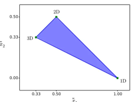
following values as the first two feature values: ˜ x1= λ1 λ1+ λ2+ λ3 , x˜2= λ2 λ1+ λ2+ λ3 .
These two values encode the shape of a distribution of points, or more especifically, its dimensionality, as shown in figure 1. Another form to exploit PCA is to interpret it as a plane fitting operation, as explained in [18]. Through this point of view, the eigenvector v3, associated to the smallest eigenvalue
λ3, represents an estimation of the surface normal. We use
the fact that the cloud is in the sensor reference frame, and flip the normal in function of the viewpoint, which is the frame’s origin. It is then possible to use the sensor-to-world
0.33 0.50 1.00 ˜x1 0.00 0.33 0.50 ˜x2 1D 2D 3D
Fig. 1: Eigenvalue features. This is the space generated by the first two feature values, which correspond to the normalized first two eigenvalues output by PCA. The feature values lie inside the closed triangle. The edges of the triangle, [1.0 0.0]T, [0.5 0.5]T and [0.3 0.3]T correspond to the cases where the 3D points are organized in pure 1D, 2D or 3D shapes, respectively. The definitive feature space is obtained after normalization, and corresponds to a translated and scaled version of this triangle.
transformation to transform the vector into the global reference frame, resulting in the global normal n = [nx ny nz]T. The
third feature value is given by the z coordinate: ˜
x3= nz.
In the 3D space, it makes no sense applying PCA on a set with less than four points, because such points will always be collinear or coplanar. Thus, during feature extraction we leave out points for which the condition NQ< 4 holds. Such points
are then also excluded from the classification. A beneficial consequence is that isolated outliers are naturally filtered out from classification.
The feature extraction process concludes with a statistical normalization step, relying on a mean µi and on a standard
deviation σi for each feature dimension i. These values are
determined during training. For every point x, for every dimension i, normalization is applied in the following manner:
xi=
˜ xi− µi
σi
.
Parts of feature extraction were implemented using tools such as Eigen [19] and Point Cloud Library (PCL) [20].
B. Intermediary Classification: GMM
The intermediary classification layer is a GMM. The GMM is a member of the family of mixture models, which as the name indicates, are models composed by mixtures of distributions. The basic goal of such a model is to represent a probability distribution, likely a complex one, by means of mixing multiple distributions. The individual distributions are called the model components.
Through feature extraction, a 3D point belonging to a point cloud is associated with a point x in the feature space. A GMM represents the distribution of x over the feature space by employing Gaussian distributions as components [15]. Let CY = {cy1, ..., cyNCY} be the set of intermediary classes,
NCY being the number of classes. The component, or class,
is indicated by the latent variable y = [y1... yNCY]
T. This is
done in the following manner: p(x) =X y p(y)p(x|y) = NCY X i=1 πiN (x|µi, Σi).
We note that y is a vector, and that we use yi to denote the
case where yi = 1 and yj = 0 for j 6= i, meaning that class
cyi is assigned to x. Each class is Gaussian, and is defined by
the following parameters: the mixing coefficient πi, the mean
µi and the covariance Σi.
Having in hands the distributions p(yi), p(x|yi) and p(x),
we can compute p(yi|x):
p(yi|x) = p(yi)p(x|yi) p(x) = πiN (x|µi, Σi) PNCY j=1 πjN (x|µj, Σj) . This is the Bayes equation. We call p(yi) the class prior
prob-abilities, p(x|yi) the likelihood and p(yi|x) the class posterior
probabilities. The computation of the posterior distribution corresponds to the inference step of classification. In our case, having obtained the posterior distribution through inference, we perform the decision step in sequence, and assign to a point the class that obtained the highest posterior probability. The GMM intermediary classes are data-oriented. They serve to capture all the different patterns that may be encoun-tered. Ideally, if the model were powerful enough, it should be able to capture, to abstract the different environmental and sensorial factors influencing the perception. By environmental factors, we refer to the variability and the clutter present in the environment, while by sensorial factors, we refer to the perception effects derived from the sensor sampling pattern.
Given a training set, the model parameters are found with the unsupervised Expectation-Maximization (EM) method. NCY, the number of classes in the GMM, or the number
of intermediary classes, should be large enough so that the GMM is able to provide a fine enough model of the patterns in the environment. Under this condition, we ensure that the corresponding intermediary classes can be grouped afterwards into meaningful final classes.
The number of classes indicate the complexity of the GMM. Increasing this number implies that the EM-based training will be slower, and that a larger amount of training data will be needed. Moreover, and perhaps most importantly, the grouping stage will be made slower, because the expert will have to look at and examine more classes. This layer is currently implemented using scikit-learn [21].
C. Final Classification: Grouping
The final classification layer is a grouping of the interme-diary classes into final classes. Viewing it purely through the point of view of classes, the set of intermediary classes is denoted by CY = {cy1, ..., cyNCY}, while the set of final
classes is denoted by CZ = {cz1, ..., czNCZ}. NCY and
NCZ respect the condition that NCZ ≤ NCY. This operation
aims at giving a single semantic interpretation to multiple intermediary classes. The semantics are ideally connected to
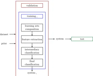
test system training i validation learning sets composition feature extraction intermediary classification final classification dataset prior system i
Fig. 3: Learning. Multiple training instances i are launched, each one resulting in a classification system i. These systems are evaluated through validation and one is selected for test. The inputs are the dataset and the prior, while the outputs are the selected system together with its test evaluation.
useful properties in a target task. We say thus that the final classes are task-oriented.
The main limitation of this method is that, in fact, not all the intermediary classes can be exploited. Some of them correspond to objects of different nature, and thus cannot be grouped into a meaningful final class. In this case, the class is marked as unknown final class. The unknown points do not contribute to the resulting semantic model. In a way, this situation is analogous to the case where, in the decision stage, we refrain from classifying a point, which is done based in some uncertainty criterion.
The grouping is determined during training. This step is done in a supervised manner, by a human expert. Overall, it consists in examining the results of the intermediary classifica-tion, by visual inspecclassifica-tion, and assigning to each intermediary class a final class, or the class unknown. This examination is performed on a grouping set, which does not have to be the same as the training set, although it usually is. To perform this task, a graphical interface is required (for this purpose, we use the ParaView visualization tool [22]). Some examples of the grouping training are shown in figure 2.
D. Learning
The learning of the full classification system follows the process of training, validation and test. A schematic overview of this process, as applied in our case, is shown in figure 3. During training, we must go through four stages: learning sets composition, feature extraction, intermediary classification and final classification. Each stage has parameters that must be determined. In a training instance, part of these parameters is manually fixed, while the other part is determined auto-matically. The result of training is a full classification system, which however might not be optimal due to the choices for the fixed parameters.
During validation, the systems resulting from multiple train-ing instances, with different parameter choices, are evaluated,
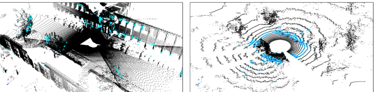
(a) Single intermediary classes that fail to represent a single element, and thus might not be grouped, depending on the target task. In the Freiburg case, it could represent either building or vegetation. In the Caylus case, it could represent either road or grass.
(b) Single intermediary classes that represent a single element, and thus are likely to be grouped. In the Freiburg case, it represents ground. In the Caylus case, it represents vegetation.
(c) Intermediary classes that are grouped into one final class. In the Freiburg case, they represent ground, while in the Caylus case, they represent vegetation.
Fig. 2: Grouping. These are examples of the actual interface used in the training process. Left: a scan from the Freiburg dataset. Right: one from the Caylus dataset. The concerned classes are highlighted in colours.
and the one with the best performance is selected. In this way, validation allows us to determine the parameters that are not automatically computed in training. The selected system is then submitted to a final evaluation in the test step.
Overall, the learning inputs are the dataset and the prior information. The dataset is the source of the actual training, validation and test sets chosen during the learning sets com-position. The prior corresponds to any assumption, hypothesis or choice made about the system. The features and the classification model, for example, are part of the prior, as well as the set of different parameters used in validation.
The learning outputs are the definitive classification system and its evaluation through the test step. The system is pre-dictive, able to classify new data, and must therefore be able to achieve a certain degree of generalization. In our work, we aim at achieving a basic level of generalization which
we call the dataset level. Generalizing at the dataset level means that the system is capable of classifying data coming from a similar environment and acquired with a similar sensor setup. Achieving higher levels of generalization would mean changing the environment or changing the sensor setup.
IV. EXPERIMENTALSETUP
The evaluation of the proposed approach follows the train-ing, validation and test steps. We evaluate the system under two separate contexts, each one corresponding to a different dataset. Both datasets contain 3D point clouds of outdoor environments. The first one is the Freiburg public dataset [3], for which we have ground-truth, made available in [5]. The second one is a dataset acquired with our own robot and sensor setup, for which there is no ground-truth available.
In each case, we train multiple systems to be compared through validation. A complete validation is a search problem, and would consist of training all the possible combinations of parameters. This leads to a combinatorial problem. In our approach, each training case includes the supervised grouping process. Due to the time required in the grouping and the combinatorial factor of the validation, it is not possible for us to proceed in an exhaustive manner.
We choose to perform a constrained validation, selecting a set of training cases considered as most informative. Con-cretely, this means testing each parameter at a time, by varying it while fixing the others at relevant values. In the end, this leads to a system which is the best locally, under the selected parameter set, yet it still leads to an informative exploration of the different alternatives. The selection of the parameters is done based on a preliminary training evaluation.
A. Freiburg Dataset
This is a public dataset, acquired at the Freiburg University’s campus [3]. It contains artificial elements such as streets, buildings of different types, road signs and lamp posts, but also some natural elements such as trees of different shapes and sizes, shrubs and vegetation areas. Some people appear in the scans too. The dataset was acquired with a SICK LMS lidar [23], [24], moved using a pan-tilt unit, on a mobile robot. The acquisition was static: the laser acquired the points while the robot was stopped. At each location, three scans at different orientations were taken and merged together. The individual scans overlap each other, creating different sampling densities at the overlapping regions.
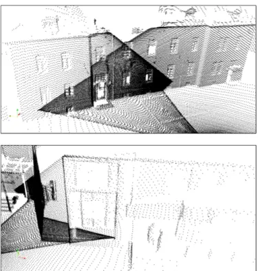
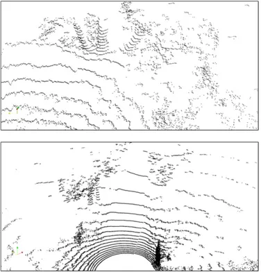
The Freiburg environment is relatively flat, structured and uncluttered. The point clouds are relatively dense. There are two main challenges encountered in the data. The first one is the nonuniform sampling, consisting of significative changes in the sampling density at the overlapping areas. The second one is the variability of facade features, such as windows, doors, roof and prominent features in general, all of them in varied sizes and types. Figure 4 shows some examples of these. The ground-truth presents a fine distinction of elements, with twenty classes in total. These include, for example, ground, sidewalk and lawn, as well as facade, window and door. These are grouped into the smaller set of final classes. We follow approximately the work done in [5], for which the ground-truth was produced, and where the classes are also grouped for the evaluation. The classes considered in their case were: ground, facade, pole and vegetation. These are relatively similar to ours, except that we include bicycles as vegetation, whereas they leave out the bicycle points from the evaluation, and that we include shrubs as facade, instead of as vegetation. The ground-truth does not cover all the points in the scans. Some complex features are left out, such as glass facades and the roofs of bicycle stations. Isolated groups of points, and some erroneous artifacts, are also filtered out. These points are thus not used in the evaluation. They are, however, still present in the training set, which means that they still contribute to the training of the model.
Fig. 4: Freiburg dataset. The top image shows a region where the individual scans overlap, causing important changes in the point densities. The bottom image shows a facade with a variety of window types.
B. Caylus Dataset
This dataset was acquired with our own robot and sensor setup, in an artificial countryside village. It presents a great variety of natural elements such as low and high grass, trees, bushes and other vegetation, but also artificial elements like an asphalted road, buildings, and some abandoned vehicles. The operator of the robot can be seen in some scans. The scans were acquired with a Velodyne HDL-32 lidar [25], mounted on the top of a Segway RMP-400-based UGV.
The Velodyne lidars, including the HDL-32, are designed to allow mobile acquisition. The dataset was acquired in this way. The UGV was manually controlled by an operator, while the lidar acquired data and a SLAM method, namely RT-SLAM [26], provided the localization by fusing GPS, inertial and visual information.
The area of the dataset presents some gentle slopes at specific points. Otherwise, it is basically flat. It is much less structured than the Freiburg area, with more grass, vegetation and some natural terrain. However, the two main challenging characteristics are the nonuniform sampling and the clutter. Here, nonuniform sampling refers to the fact that the sampling is relatively dense at close ranges, but becomes more and more sparse at farther ranges. This effect is normally present in scans from any lidar, but it is specially pronounced in the case of the Velodyne. As a result, it constitutes a bigger factor in the scans from the Velodyne, in Caylus, than in the scans from the SICK, in Freiburg. As for clutter, the second challenge, it is present in important amounts in the Caylus environment, and concerns particularly tree trunks, often surrounded by vegetation. Figure
Fig. 5: Caylus dataset. The top image shows an example of clutter found in the set. At the top-left of it, we can see two tree trunks being surrounded by foliage and vegetation. The bottom image shows the sampling sparsity problem. It is particularly noticeable for the road, going from the bottom-center to the top-center of the image, and presenting a dramatic decrease in sampling.
5 shows examples of both phenomena. C. Metrics
The Freiburg dataset contains ground-truth data, therefore allowing a quantitative evaluation. We choose to use the precision, recall and F1 metrics, as shown in table I. These
metrics take into account the classwise performance, which is necessary when dealing with unbalanced data, as is the case in semantic modelling. Moreover, F1 produces a generic
evaluation because it includes both precision and recall. For certain target tasks, it might be desirable to prioritize either precision or recall, and then other metrics can be used. The total F1 score is computed as F1total =
1 NCZ
P
iF1i, F1i
indicating the classwise F1score. The accuracy metric is also
reported.
For the Caylus dataset, there is no associated ground-truth. Actually, this is an example of a dataset for which ground-truth is difficult to produce, due to two factors: the sampling sparsity and the presence of more natural, non-structured elements. The evaluation, in this case, is done only in a qualitative manner, by visual inspection. This case represents a real implementation of our system, starting from a dataset with no ground-truth, and ending with a visual inspection of the classification results. We note that the relative difference in recall between differ-ent scans can be convenidiffer-ently noticed. It is, most of the times, clear enough to see missing points in one scan, compared
to another. Therefore, the evaluation is done in a relative way. Scans are compared between them, and differences on the recalls are noted down. This allows a ranking to be established. This procedure is consistent with the grouping method adopted, which also prioritizes the recall. The actual criterion used in the visual evaluation would depend on the target task, and could possibly prioritize different factors, other than the recall.
V. EVALUATION
The implementation of the evaluation method is done by defining one validation and one test sets. The training set, however, may vary in each training case. The validation set is used to evaluate every training case, while the test set is used to evaluate the selected system.
From each dataset, 10 scans were reserved for use in the different training sets, 5 for the validation set and 5 for the test set. The training scans were the first ones to be chosen, followed by the validation scans, and finally by the test scans. Assigning the priorities in this manner ensures that the system will learn with the best data available. The selected scans were kept as spread as possible over the scenes, while at the same time being picked from the most interesting areas, and aiming at having as much balance as possible between the different elements.
A. Preliminary Training Evaluation
The preliminary training evaluation uses all the scans re-served for training. It allows us to select the parameters to be evaluated in the validation. Three different training are selected, containing respectively 2, 5 and 10 scans, picked from the training scans. The feature parameters, r and R, are also evaluated. Five different values of r are considered, 0.2m, 0.4m, 0.6m, 0.8m and 1.0m, as well as a multi-scale version with R = {0.2m, 0.4m, 0.6m, 0.8m, 1.0m}. Another evaluated parameter is the number of intermediary classes, NCY. Using 50 classes is considered to be the maximum
number acceptable, because higher numbers would make the grouping training slower, and therefore too cumbersome. We thus test models with 10, 30 and 50 classes.
The final classes were not manually pre-selected, but in-stead, discovered on the preliminary training evaluation. For the Freiburg dataset, the set of final classes is composed by four classes. They were checked against the ground-truth available, to ensure that the latter could be used to support the evaluation. The classes are the following:
• ground. It corresponds to road, lawn, sidewalks, and so
on. Geometrically, these are flat and planar, with normals oriented upwards.
• building. It corresponds to buildings, including any facade structure, roofs, and so on, and also to shrubs. Shrubs are included here because they are so precisely trimmed that they appear clearly as low walls. Only in scarce cases, some edges present random traces indicating vegetation. Geometrically, the facades and shrubs are planar with normals oriented along the horizontal plane, whereas the facade structures have more varied geometries.
unk cz1 ... czi ... czNCZ rec F1 cz1 f pi,1 . . . . . .
czi f ni,unk f ni,1 ... tpi ... f ni,NCZ reci F1i
. . . . . . czNCZ f pi,NCZ
pre - prei - F1total
Evaluation metrics. This table shows the confusion matrix, with added information about the precision, recall and F1scores. The rows indicate the true classes, while the columns indicate the predicted classes. unk refers to the unknown final class, czito the i-th final class, pre to precision, and rec to
recall. tp indicates the true positives, f p the false positives, and f n the false negatives.
TABLE I
• trunk. It corresponds to tree trunks, posts and people. Geometrically, these are linear, with normals oriented along the horizontal plane.
• vegetation. It corresponds to vegetation, tree foliage and to bicycles and bicycle stations too. Parked bicyles and bicyles stations are common in the dataset, and their relatively random and scatteered shape matches well that of vegetation in general, therefore being included here. Geometrically, they are scattered, three-dimensional, with normals oriented in unpredictable directions.
For the Caylus dataset, after the preliminary training eval-uation, the set of final classes was composed by the six discovered classes:
• road. It corresponds to the asphalted road, and to side-walks. Geometrically, these are planar, with normals oriented upwards.
• building. It corresponds to buildings and facade features,
such as doors and windows. Geometrically, these are planar, with normals oriented along the horizontal plane, except from the facade features which have varied ge-ometries.
• trunk. It corresponds to tree trunks, posts and people. Posts are rare, but still present in the dataset. People refers mainly to the robot operator who appears in most of the scans. Geometrically, these are linear, with normals oriented mainly horizontally, but sometimes in other directions, for example when a trunk is inclined.
• vegetation. It corresponds to tree foliage and vegetation. Some regions where the grass is high can be considered as vegetation too. Geometrically, these are scattered, three-dimensional.
• grass. It corresponds to grass. Geometrically, it is
ba-sically planar, but less than road, because of the more scattered pattern of the grass.
• rough. It corresponds to rough terrain, usually found at the interface of grass and vegetation, or at the base of trees. It also corresponds to regions of medium-high grass. In fact, the classes grass, rough and vegetation represent a progression of unstructured terrain, and of scatterness, in terms of geometric shape.
B. Freiburg Test Results
We now consider the systems which performed the best in the validation stage, and submit them to the last step of evaluation: the test. From the validation results, we retrieve
that the setup which obtained the best performance was {2-scan-training-set, r = 0.6m, NCY = 50}. In the set of
final classes, {ground, building, trunk, vegetation}, ground has the purest semantic interpretation. building includes shrubs too, as previously explained. trunk includes posts and people. vegetation includes bicycles. Therefore, these classes mix elements of different nature, to some extent. There is, however, a consistent point underlying them, discussed previously in their presentation: the geometry. A definitive judgement on the semantic interpretation of the discovered classes depends on the target task. In the case where geometry constitutes the required information, these classes can be considered relevant. Otherwise, a finer classification system would be necessary, one that could for instance join shrubs to vegetation, and exclude bicycles from vegetation. Such a finer system would require as input more specific, detailed geometric representations, or other types of information such as vision or information from a knowledge-base.
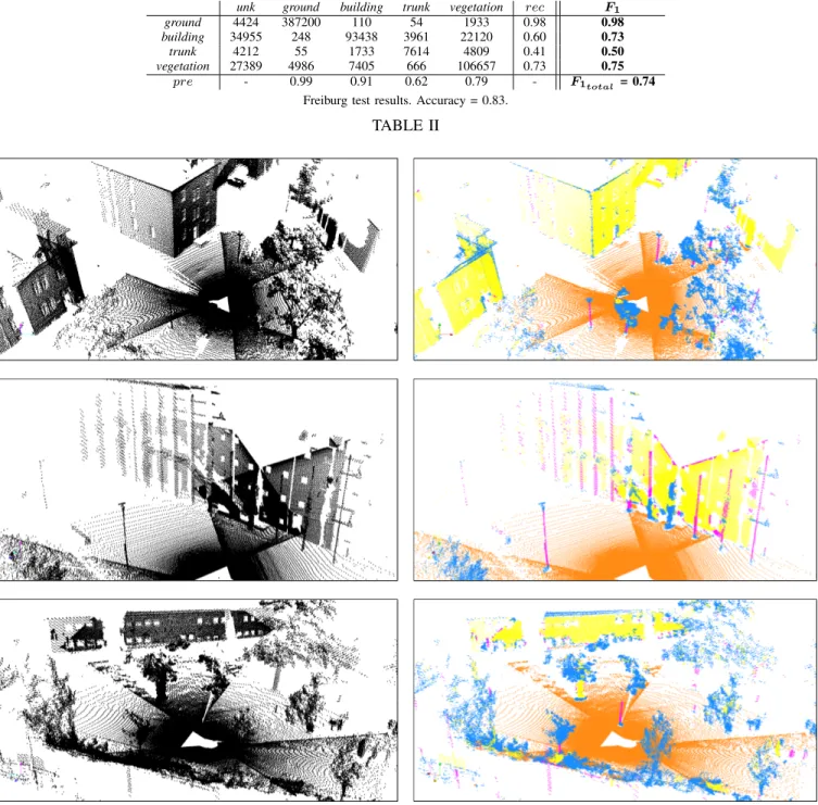
Table II shows the quantitative results of the test. Figure 6 shows the classification on the test scans. The total F1obtained
is 0.74. It is lower than the score obtained in the validation step, 0.77, yet close enough to confirm that the system was able to generalize from the validation set to the test set. A generalization at the dataset level, in this case, is therefore verified.
In order to increase the performance, the complexity of the system must be increased, by either using a more complex feature extraction stage or a more complex classification stage. Regarding the feature extraction, the selected system already presents the feature parameters that obtained the best performance, so the feature extraction process itself must be improved. As for the number of intermediary classes, since it is already at its maximum, complexifying the classification model means changing the model itself.
As for the remaining of the test scores, we can note that the precision scores are all higher than the recall scores. The main reason behind this difference is the impossibility of using all the intermediary classes provided by the GMM, leaving some of them as unknown. This can be observed in the results: apart from the case of the class trunk, the highest number of false negatives always appears under unknown. This is a characteristic of our two-layer approach: the data-oriented, intermediary layer learns the different patterns encountered in the data, but the task-oriented, final layer discards those which fail to correspond to some meaningful semantics.
unk ground building trunk vegetation rec F1 ground 4424 387200 110 54 1933 0.98 0.98 building 34955 248 93438 3961 22120 0.60 0.73 trunk 4212 55 1733 7614 4809 0.41 0.50 vegetation 27389 4986 7405 666 106657 0.73 0.75 pre - 0.99 0.91 0.62 0.79 - F1total = 0.74
Freiburg test results. Accuracy = 0.83.
TABLE II
Fig. 6: Freiburg classification test results. Input at the left, output at the right. Colours: (ground, orange), (building, yellow), (trunk, pink), (vegetation, blue). The misclassification of some facade regions as vegetation can be seen in some of the scans, as well as the misclassification of the base of posts as vegetation.
Classwise, ground obtained the best F1, precision and
recall scores. This is understandable, because in the struc-tured Freiburg environment, the ground can be consistently distinguished due to its planar shape and upwards normal orientation. trunk obtained the worst scores. It is confused with borders of other objects, especially corners of buildings, windows and doors. Additionally, the base and the top of tree trunks, as well as the base of posts, are frequently misclassified as vegetation. This factor can be spotted in the confusion matrix, appearing as the high number of vegetation false positives actually corresponding to trunk. In all these
cases, the confusions between trunk and building or vegetation have a greater negative effect on trunk, because of its rarity. vegetationsuffers from misclassifications too, being confused with elements such as corners and roofs of buildings.
The limitations encountered are, in a way, due to the important density changes present in the data. Such changes make the distinctions harder by multiplying the patterns cor-responding to each element. However, this point is addressed in part through the set of intermediary classes, which are able to represent some of the different patterns. Overall, the main problem seems to lie in the variability of the facade features,
such as windows, doors, roofs, prominent regions, corners and so on. These are the elements most frequently misclassified, either as post or vegetation, irrespective of sampling densities. The main source of this problem, in turn, are the features employed, which do not allow a better distinction of the elements.
C. Caylus Test Results
In the validation, the setup which obtained the best perfor-mance was {10-scan-set, r = 0.6m, NCY = 50}. The set of
final classes, {road, building, trunk, vegetation, grass, rough}, is larger than the Freiburg set. road, building and grass have the purest semantic interpretations. trunk includes the road, posts and people. vegetation includes high grass, bushes and foliage. rough includes rough terrain, such as stony ground, and medium grass. As in the Freiburg case, the common underlying link is the geometry. It is interesting to note that the classes ground, grass, rough and vegetation can be interpreted as a progression in terms of scatterness of the geometry, while, to some extent, still correspond to specific elements in the environment.
Similarly to the Freiburg case, the test performance matched the validation performance, so the system was able to gen-eralize to the test set, confirming its capacity to achieve a dataset-level generalization. As for Freiburg, the results corre-spond to the system complexity. Because the best parameters were already determined through the validation, increasing the performance would require a change in the feature extraction stage or in the classification stage.
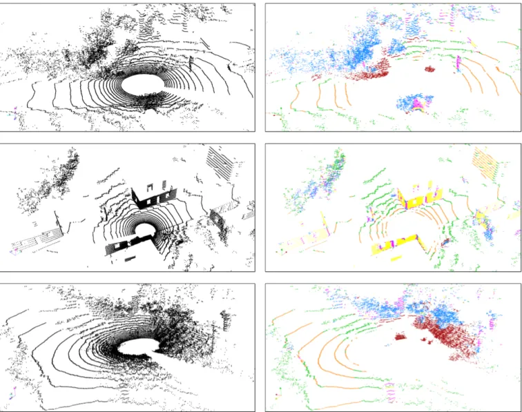
Figure 7 shows the classification results on the scans of the test set. The main problem is the non-distinction of the nearest points to the sensor, which correspond either to the road or to grass. In other words, the system was unable to separate nearby road from nearby grass. Another problem was that, at far range, vegetation was perceived as grass. Yet another difficulty encountered was also present in the Freiburg dataset: the confusion between vegetation, trunks and building features. In the Caylus case, however, this effect was more constrained. Firstly, because the Caylus facades are sampled in a relatively similar manner, while the Freiburg facades are sampled in a variety of ways due to the overlapping scans. Secondly, because the Caylus facade features are simpler, corresponding to simple squared windows and doors.
The nonuniform sampling in the data impacted the dis-tinction between distant road and distant buildings. At far range, because of the line-based sampling pattern of the Velodyne lidar, these two elements appear simply as lines, therefore having the same shape and normals oriented along unpredictable directions. The sampling also played a part in the confusion between distant vegetation and grass. Were the sampling is denser, these two elements would maybe have been better distinguished. Clutter, on the other side, affected the classification of trunks, as many were considered as vegetation because they were entirely surrounded by it.
In the end, among the class confusions, the nonuniform sampling effects, and the clutter, the main source of difficulty remains the class confusions: nearby road with grass, distant
vegetation with grass, buildings with trunks and vegetation. These, in turn, are a consequence of the feature representation used. Thus, as happened in the Freiburg case, the features do not allow a better distinction between these elements.
VI. CONCLUSION
The approach proposed in this work takes as input a 3D point cloud with its corresponding sensor-to-world transforma-tion, and outputs a classified version of the point cloud. The feature extraction represents the shape of a point neighbour-hood using information from a PCA operation. Regarding the classifier, the first, intermediary layer corresponds to a GMM trained in an unsupervised manner, and the second, final layer corresponds to a grouping of the intermediary classes into final classes. The approach avoids the necessity of manually labelling the input dataset, instead requiring a manual training of the grouping which is based on the trained intermediary layer.
The evaluations show that the approach is able to achieve a dataset generalization. The main advantages are the following: + Data-orientation. The unsupervised training of the GMM brings the data-oriented aspect to the system. The GMM classes are able to capture, at least in part, the variety of patterns in the data, addressing challenges such as nonuniform sampling, sensor noise, environment variabil-ity and clutter in an unsupervised manner.
+ Task-orientation. In spite of its unsupervised core, the approach is able to deliver final classes which, under certain conditions, can be semantically interpreted. In all cases, the final classes are consistent with the geometry represented through the features. The final classes are defined with the grouping, which brings the task-oriented aspect, in a principled and explicit manner. The system can be used as a predictive model in a target task. + Standard design and operation. The design follows a
stan-dard learning procedure with a training, a validation and a test steps. The operation follows a standard classification pipeline. It is composed by a feature extraction and a classification stages. The classification stage groups the elementary stages of inference and decision.
+ Simplicity. There is no requirement of pre-processing or post-processing stages, although these may be included. The feature extraction and classification stages are simple. The design procedure, mainly based on unsupervised learning, is simple.
The main disadvantages are the following:
- Training noise. This refers to two factors. The first is the randomness present in the GMM training due to the random initialization method, constituting the GMM training noise. The second is the randomness present in the grouping training layer due to the expert supervision process, which is bound to be erroneous from time to time, constituting the grouping noise. They both con-stitute the training noise. Such noise is a disadvantage because it affects the final classification performance, which ideally would be deterministic and predictable in all cases.
Fig. 7: Caylus classification test results. Input at the left, output at the right. Colours: (road, orange), (building, yellow), (trunk, pink), (vegetation, blue), (grass, green), (rough, brown). The missing nearby points can be clearly detected in the scans. Some misclassifications of building features as trunk can also be observed.
- Supervision computational complexity. The approach re-quires a supervised training of the grouping, which is done for each system evaluated in the learning process. In terms of computational complexity, this corresponds to a linear complexity. A supervised approach, on the contrary, requires a single, supervised labelling of the input dataset, offering a lower computational complexity. If taken individually, on the other hand, the grouping training is much simpler than the dataset labelling, be-cause it is guided by the intermediary classes discovered by the GMM.
- Final performance. Considering the simplicity of the system, the performance is reasonable. With respect to the state-of-the-art, however, it does not compete with more advanced classification systems.
Between the feature extraction, the intermediary GMM and the final grouping, the feature extraction constitutes the main factor limiting the performance of the approach. In
this context, a first extension could be the addition of an extra feature value, x4, coming also from the PCA operation:
the z coordinate of the world-frame representation of v2,
the second PCA eigenvector. This value can be seen as the natural complement for the current value x3, which is the z
coordinate of the world-frame representation of the normal, or v3. This would add one extra dimension of information about
the orientation of the points. It would allow, for instance, to isolate vertical linear elements such as vertical tree trunks and posts, with x3 and x4 being both zero in this case.
It would be interesting to test the approach under an application case. A natural case would be terrain traversability analysis. A rough scheme of how our system can be used in such context is given hereafter. The final classes are each linked to a traversability class, which in turn are each linked to a traversability cost. The output pointwise structure is trans-formed to a 3D-voxel model. Under a conservative criterion, the class of a voxel may be set as the highest-cost class among
the classes of the individual points within the voxel. For a 2D path planning, the voxels above a certain height may be ignored, and the others projected onto a subsequent 2D-grid model, using the same conservative criterion. For a 3D path planning, the 3D-voxel model would already be enough. The classes of the final model, corresponding to traversability costs, would provide the cost criterion for a path planning algorithm. As an example, we consider the model produced for the Caylus dataset as being appropriate to tackle such a problem in that environment.
Besides terrain traversability analysis, the proposed ap-proach may also be useful in a number of other cases. An example is the rapid production of an operational semantic model in a case of search and rescue. The simplicity of design of the system would be advantageous. The model produced could be used as a preliminary but operational model, while maybe a finer, more complete model would be put under construction. Another example is the comparison of different classification systems. In this case, our system could be used as a baseline reference in the comparison, its simple and unsupervised nature allowing it to be rapidly designed. Yet another example is the labelling of a dataset, or equivalently, the production of a ground-truth, which, after all, was one of the main concerns behind this work. Because our system is unsupervised at its core, it can justly be used as an aid in the full labelling of a dataset. Lastly, our approach can, of course, be used in any case where it already provides a fine-enough model for the required target task.
REFERENCES
[1] P. Papadakis, “Terrain traversability analysis methods for unmanned ground vehicles: A survey,” Engineering Applications of Artificial In-telligence, vol. 26, no. 4, 2013.
[2] M. Himmelsbach, T. Luettel, and H. Wuensche, “Real-time object classification in 3d point clouds using point feature histograms,” in IROS, 2009.
[3] B. Steder, M. Ruhnke, S. Grzonka, and W. Burgard, “Place recognition in 3d scans using a combination of bag of words and point feature based relative pose estimation,” in IROS, 2011.
[4] A. N¨uchter and J. Hertzberg, “Towards semantic maps for mobile robots,” Robotics and Autonomous Systems, vol. 56, no. 11, 2008. [5] J. Behley, V. Steinhage, and A. Cremers, “Performance of histogram
descriptors for the classification of 3d laser range data in urban envi-ronments,” in ICRA, 2012.
[6] F. Moosmann and M. Sauerland, “Unsupervised discovery of object classes in 3d outdoor scenarios,” in IEEE International Conference on Computer Vision Workshops (ICCV Workshops), 2011.
[7] J.-F. Lalonde, N. Vandapel, D. Huber, and M. Hebert, “Natural terrain classification using three-dimensional ladar data for ground robot mo-bility,” Journal of Field Robotics, vol. 23, no. 10, 2006.
[8] E. Lim and D. Suter, “3d terrestrial lidar classifications with super-voxels and multi-scale conditional random fields,” Computer-Aided Design, vol. 41, no. 10, 2009.
[9] N. Brodu and D. Lague, “3d terrestrial lidar data classification of complex natural scenes using a multi-scale dimensionality criterion: Applications in geomorphology,” ISPRS Journal of Photogrammetry and Remote Sensing, vol. 68, no. 0, 2012.
[10] F. Moosmann, O. Pink, and C. Stiller, “Segmentation of 3d lidar data in non-flat urban environments using a local convexity criterion,” in IEEE Intelligent Vehicles Symposium, 2009.
[11] A. Aijazi, P. Checchin, and L. Trassoudaine, “Segmentation based classification of 3d urban point clouds: A super-voxel based approach with evaluation,” Remote Sensing, vol. 5, no. 4, 2013.
[12] D. Munoz, N. Vandapel, and M. Hebert, “Onboard contextual classifica-tion of 3-d point clouds with learned high-order markov random fields,” in ICRA, 2009.
[13] R. Triebel, R. Paul, D. Rus, and P. Newman, “Parsing outdoor scenes from streamed 3d laser data using online clustering and incremental belief updates,” in AAAI Conference on Artificial Intelligence, 2012. [14] M. Ruhnke, B. Steder, G. Grisetti, and W. Burgard, “Unsupervised
learning of compact 3d models based on the detection of recurrent structures,” in IROS, 2010.
[15] C. Bishop, Pattern Recognition and Machine Learning. Springer-Verlag New York, Inc., 2006.
[16] R. Unnikrishnan, “Statistical approaches to multi-scale point cloud processing,” Ph.D. dissertation, Robotics Institute, Carnegie Mellon University, 2008.
[17] F. Neuhaus, D. Dillenberger, J. Pellenz, and D. Paulus, “Terrain driv-ability analysis in 3d laser range data for autonomous robot navigation in unstructured environments,” in ETFA, 2009.
[18] K. Klasing, D. Althoff, D. Wollherr, and M. Buss, “Comparison of surface normal estimation methods for range sensing applications,” in IEEE International Conference on Robotics and Automation (ICRA), 2009.
[19] G. Guennebaud, B. Jacob, et al., “Eigen v3,” http://eigen.tuxfamily.org, 2013.
[20] R. Rusu and S. Cousins, “3d is here: Point cloud library (PCL),” in IEEE International Conference on Robotics and Automation (ICRA), 2011. [21] F. Pedregosa, G. Varoquaux, A. Gramfort, V. Michel, B. Thirion,
O. Grisel, M. Blondel, P. Prettenhofer, R. Weiss, V. Dubourg, J. Vander-plas, A. Passos, D. Cournapeau, M. Brucher, M. Perrot, and E. Duch-esnay, “Scikit-learn: Machine learning in Python,” Journal of Machine Learning Research, vol. 12, pp. 2825–2830, 2011.
[22] K. Moreland, “The paraview tutorial,” Sandia National Laboratories, Tech. Rep., 2013.
[23] SICK, “Lms200-30106,” Datasheet, 2015. [24] ——, “Lms291-s05,” Datasheet, 2015.
[25] Velodyne, “Hdl-32e,” User’s Manual, Revision E, 2012.
[26] C. Roussillon, A. Gonzalez, J. Sol`a, J.-M. Codol, N. Mansard, S. Lacroix, and M. Devy, “Rt-slam: A generic and real-time visual slam implementation,” in Computer Vision Systems. Springer, 2011, vol. 6962, pp. 31–40.
Artur Maligo received his PhD from LAAS/CNRS. There, he worked in the field robotics team, and his research covered semantic modelling based on 3D lidar data. Overall, he is interested in using machine learning methods to solve the classification problem. He focuses in using unsupervised learning to ease the learning process.
Simon Lacroix is a research scientist at LAAS/CNRS, where he animates the field robotics activities. He was mainly involved in planetary robotics during the 90’s, and has initiated aerial robotics activities in the lab in the beginning of the 2000’s. Since then, his research is focused on the deployment of teams of multiple heterogeneous autonomous robots for exploration, surveillance or intervention missions. His main interests originally concerned perception and navigation for autonomous aerial and terrestrial robots (environment perception and modeling, localisation, perception control and autonomous navigation strategies), and have evolved towards decisional processes required by the cooperation within multi-robot teams.