Anomalous transport in disordered fracture networks: Spatial
Markov model for dispersion with variable injection modes
The MIT Faculty has made this article openly available. Please share
how this access benefits you. Your story matters.
Citation Kang, Peter K. et al. "Anomalous transport in disordered fracture
networks: Spatial Markov model for dispersion with variable
injection modes." Advances in Water Resources 106 (August 2017): 80-94 © 2017 Elsevier
As Published http://dx.doi.org/10.1016/j.advwatres.2017.03.024
Publisher Elsevier BV
Version Original manuscript
Citable link https://hdl.handle.net/1721.1/123817
Terms of Use Creative Commons Attribution-NonCommercial-NoDerivs License
Anomalous transport in disordered fracture networks:
spatial Markov model for dispersion with variable
injection modes
Peter K. Kang
Korea Institute of Science and Technology, Seoul 02792, Republic of Korea Massachusetts Institute of Technology, 77 Massachusetts Ave, Building 1, Cambridge,
Massachusetts 02139, USA Marco Dentz
Institute of Environmental Assessment and Water Research (IDÆA), Spanish National Research Council (CSIC), 08034 Barcelona, Spain
Tanguy Le Borgne
Universit´e de Rennes 1, CNRS, Geosciences Rennes, UMR 6118, Rennes, France Seunghak Lee
Korea Institute of Science and Technology, Seoul 02792, Republic of Korea Ruben Juanes
Massachusetts Institute of Technology, 77 Massachusetts Ave, Building 1, Cambridge, Massachusetts 02139, USA
Abstract
We investigate tracer transport on random discrete fracture networks that are characterized by the statistics of the fracture geometry and hydraulic conductivity. While it is well known that tracer transport through fractured media can be anomalous and particle injection modes can have major im-pact on dispersion, the incorporation of injection modes into effective trans-port modelling has remained an open issue. The fundamental reason behind
this challenge is that—even if the Eulerian fluid velocity is steady—the La-grangian velocity distribution experienced by tracer particles evolves with time from its initial distribution, which is dictated by the injection mode, to a stationary velocity distribution. We quantify this evolution by a Markov model for particle velocities that are equidistantly sampled along trajecto-ries. This stochastic approach allows for the systematic incorporation of the initial velocity distribution and quantifies the interplay between veloc-ity distribution and spatial and temporal correlation. The proposed spatial Markov model is characterized by the initial velocity distribution, which is determined by the particle injection mode, the stationary Lagrangian veloc-ity distribution, which is derived from the Eulerian velocveloc-ity distribution, and the spatial velocity correlation length, which is related to the characteristic fracture length. This effective model leads to a time-domain random walk for the evolution of particle positions and velocities, whose joint distribution follows a Boltzmann equation. Finally, we demonstrate that the proposed model can successfully predict anomalous transport through discrete fracture networks with different levels of heterogeneity and arbitrary tracer injection modes.
Keywords: Discrete Fracture Networks, Injection Modes, Anomalous
Transport, Stochastic Modelling, Lagrangian Velocity, Time Domain Random Walks, Continuous Time Random Walks, Spatial Markov Model
1. Introduction 1
Flow and transport in fractured geologic media control many impor-2
tant natural and engineered processes, including nuclear waste disposal, ge-3
ologic carbon sequestration, groundwater contamination, managed aquifer 4
recharge, and geothermal production in fractured geologic media [e.g., 1, 5
2, 3, 4, 5]. Two dominant approaches exist for simulating flow and trans-6
port through fractured media: the equivalent porous medium approach [6, 7] 7
and the discrete fracture network approach (DFN) [8, 9, 10, 11, 12, 13, 14, 8
15, 16, 17, 18, 19, 20, 21]. The DFN approach explicitly resolves individ-9
ual fractures whereas the equivalent porous medium approach represents 10
the fractured medium as a single continuum by deriving effective parame-11
ters to include the effect of the fractures on the flow and transport. The 12
latter, however, is hampered by the fact that a representative elementary 13
volume may not exist for fractured media [22, 23]. Dual-porosity
mod-14
els are in between these two approaches, and conceptualize the fractured-15
porous medium as two overlapping continua, which interact via an exchange 16
term [24, 25, 26, 27, 28, 29, 30, 31, 32]. 17
DFN modelling has advanced significantly in recent years with the in-18
crease in computational power. Current DFN simulators can take into ac-19
count multiple physical mechanisms occurring in complex 3D fracture sys-20
tems. Recent studies also have developed methods to explicitly model ad-21
vection and diffusion through both the discrete fractures and the permeable 22
rock matrix [33, 34, 35, 36]. In practice, however, their application must 23
account for the uncertainty in the subsurface characterization of fractured 24
media, which is still an considerable challenge [37, 38, 39]. Thus, there is a 25
continued interest in the development of upscaled transport models that can 26
be parameterized with a small number of model parameters. Ideally, these 27
model parameters should have a clear physical interpretation and should be 28
determined by means of field experiments, with the expectation that the 29
model can then be used for predictive purposes [40, 41]. 30
Developing an upscaled model for transport in fractured media is espe-31
cially challenging due to the emergence of anomalous (non-Fickian) trans-32
port. While particle spreading is often described using a Fickian framework, 33
anomalous transport—characterized by scale-dependent spreading, early ar-34
rivals, long tails, and nonlinear scaling with time of the centered mean 35
square displacement—has been widely observed in porous and fractured 36
media across multiple scales, from pore [42, 43, 44, 45, 46] to single frac-37
ture [47, 48, 49, 50] to column [51, 52] to field scale [53, 54, 55, 56, 57, 41, 58]. 38
The ability to predict anomalous transport is essential because it leads to fun-39
damentally different behavior compared with Fickian transport [59, 60, 61]. 40
The continuous time random walk (CTRW) formalism [62, 63] is a frame-41
work to describe anomalous transport through which models particle motion 42
through a random walk in space and time characterized by random space 43
and time increments, which accounts for variable mass transfer rates due 44
to spatial heterogeneity. It has been used to model transport in heteroge-45
neous porous and fractured media [64, 65, 66, 67, 68, 49, 69] and allows 46
incorporating information on flow heterogeneity and medium geometry for 47
large scale transport modelling. Similarly, the time-domain random walk 48
(TDRW) approach [70, 71, 72] models particle motion due to distributed 49
space and time increments, which are derived from particle velocities and 50
their correlations. The analysis of particle motion in heterogeneous flow
51
fields demonstrate that Lagrangian particle velocities exhibit sustained cor-52
relation along their trajectory [73, 70, 74, 75, 76, 77, 78, 79, 45]. Volume 53
conservation induces correlation in the Eulerian velocity field because fluxes 54
must satisfy the divergence-free constraint. This, in turn, induces correlation 55
in the Lagrangian velocity along a particle trajectory. To take into account 56
velocity correlation, Lagrangian models based on Markovian processes have 57
been proposed [70, 71, 74, 76, 77, 78, 45, 41, 80]. Spatial Markov models 58
are based on the observation that successive velocity transitions measured 59
equidistantly along the mean flow direction exhibit Markovianity: a parti-60
cle’s velocity at the next step is fully determined by its current velocity. The 61
spatial Markov model, which accounts for velocity correlation by incorporat-62
ing this one-step velocity correlation information, has not yet been extended 63
to disordered (unstructured) DFNs. 64
The mode of particle injection can have a major impact on transport 65
through porous and fractured media [81, 82, 83, 84, 85, 86, 58, 87]. Two 66
generic injection modes are uniform (resident) injection and flux-weighted 67
injection with distinctive physical meanings as discussed in Frampton and 68
Cvetkovic [84]. The work by Sposito and Dagan [82] is one of the earliest 69
studies of the impact of different particle injection modes on the time evolu-70
tion of a solute plume spatial moments. The significance of injection modes 71
on particle transport through discrete fracture networks has been studied for 72
fractured media [84, 58]. Dagan [87] recently clarified the theoretical relation 73
between injection modes and plume mean velocity. Despite recent advances 74
regarding the significance of particle injection modes, the incorporation of 75
injection methods into effective transport modelling is still an open issue 76
[84]. The fundamental challenge is that the Lagrangian velocity distribution 77
experienced by tracer particles evolves with time from its initial distribution 78
which is dictated by the injection mode to a stationary velocity distribution 79
[73, 84, 75, 88]. In this paper, we address these fundamental questions, in 80
the context of anomalous transport through disordered DFNs. 81
The paper proceeds as follows. In the next section, we present the studied 82
random discrete fracture networks, the flow and transport equations and 83
details of the different particle injection rules. In Section 3, we investigate the 84
emergence of anomalous transport by direct Monte Carlo simulations of flow 85
and particle transport. In Section 4, we analyze Eulerian and Lagrangian 86
velocity statistics to gain insight into the effective particle dynamics and 87
elucidate the key mechanisms that lead to the observed anomalous behavior. 88
In Section 5, we develop a spatial Markov model that is characterized by the 89
initial velocity distribution, probability density function (PDF) of Lagrangian 90
velocities and their transition PDF, which are derived from the Monte Carlo 91
simulations. The proposed model is in excellent agreement with direct Monte 92
Carlo simulations. We then present a parsimonious spatial Markov model 93
that quantifies velocity correlation with a single parameter. The predictive 94
capabilities of this simplified model are demonstrated by comparison to the 95
direct Monte Carlo simulations with arbitrary injection modes. In Section 6, 96
we summarize the main findings and conclusions. 97
2. Flow and Transport in Discrete Random Fracture Networks 98
2.1. Random Fracture Networks 99
We numerically generate random DFNs in two-dimensional rectangular 100
regions, and solve for flow and tracer transport within these networks. The 101
fracture networks are composed of linear fractures embedded in an imper-102
meable rock matrix. The idealized 2D DFN realizations are generated by 103
superimposing two different sets of fractures, which leads to realistic discrete 104
fracture networks [89, 67]. Fracture locations, orientations, lengths and hy-105
draulic conductivities are generated from predefined distributions, which are 106
assumed to be statistically independent: (1) Fracture midpoints are selected 107
randomly over the domain size of Lx×Ly where Lx = 2 and Ly = 1; (2)
Frac-108
ture orientations for two fracture sets are selected randomly from Gaussian 109
distributions, with means and standard deviation of 0◦± 5◦ for the first set,
110
and 90◦ ± 5◦ for the second set; (3) Fracture lengths are chosen randomly
111
from exponential distributions with mean Lx/10 for the horizontal fracture
112
set and mean Ly/10 for the vertical fracture set; (4) Fracture conductivities
113
are assigned randomly from a predefined log-normal distribution. An exam-114
ple of a random discrete fracture network with 2000 fractures is shown in 115
Figure 1. 116
The position vector of node i in the fracture network is denoted by xi.
The link length between nodes i and j is denoted by lij. The network is
char-acterized by the distribution of link lengths pl(l) and hydraulic conductivity
K. The PDF of link lengths here is exponential pl(l) =
exp(−l/¯l)
¯
l . (1)
Note that the link length and orientation are independent. The character-117
istic fracture link length is obtained by taking the average of a link length 118
over all the realizations, which gives ¯l ≈ Lx/200. A realization of the
ran-119
dom discrete fracture network is generated by assigning independent and 120
identically distributed random hydraulic conductivities Kij > 0 to each link
121
between nodes i and j. Therefore, the Kij values in different links are
correlated. The set of all realizations of the spatially random network gener-123
ated in this way forms a statistical ensemble that is stationary and ergodic. 124
We assign a lognormal distribution of K values, and study the impact of 125
conductivity heterogeneity on transport by varying the variance of ln(K). 126
We study log-normal conductivity distributions with four different variances: 127
σlnK = 1, 2, 3, 5. The use of this particular distribution is motivated by the
128
fact that conductivity values in many natural media can be described by a 129
lognormal law [90, 91]. 130
2.2. Flow Field 131
Steady state flow through the network is modeled by Darcy’s law [22] for 132
the fluid flux uij between nodes i and j, uij = −Kij(Φj − Φi)/lij, where Φi
133
and Φj are the hydraulic heads at nodes i and j. Imposing flux conservation
134
at each node i, P
juij = 0 (the summation is over nearest-neighbor nodes),
135
leads to a linear system of equations, which is solved for the hydraulic heads 136
at the nodes. The fluid flux through a link from node i to j is termed
137
incoming for node i if uij < 0, and outgoing if uij > 0. We denote by eij the
138
unit vector in the direction of the link connecting nodes i and j. 139
We study a uniform flow setting characterized by constant mean flow in the positive x-direction parallel to the principal set of factures. No-flow conditions are imposed at the top and bottom boundaries of the domain, and fixed hydraulic head at the left (Φ = 1) and right (Φ = 0) boundaries. The overbar in the following denotes the ensemble average over all network realizations. The one-point statistics of the flow field are characterized by the Eulerian velocity PDF, which is obtained by spatial and ensemble sampling
of the velocity magnitudes in the network pe(u) = P i>jlijδ(u− uij) N`¯l . (2)
where N` is the number of links in the network. Link length and flow
veloc-ities here are independent. Thus, the Eulerian velocity PDF is given by pe(u) = 1 N` X i>j δ(u− uij). (3)
Even though the underlying conductivity field is uncorrelated, the mass con-140
servation constraint together with heterogeneity leads to the formation of 141
preferential flow paths with increasing network heterogeneity [92, 80]. This 142
is illustrated in Figures 2a and b, which show maps of the relative velocity 143
magnitude for high velocities in networks with log-K variances of 1 and 5. As 144
shown in Figures 2c and d, for low heterogeneity most small flux values occur 145
along links perpendicular to the mean flow direction, whereas low flux values 146
do not show directionality for the high heterogeneity case. This indicates 147
that fracture geometry dominates small flux values for low heterogeneity and 148
fracture conductivity dominates small flux values for high heterogeneity. An 149
increase in conductivity heterogeneity leads to a broader Eulerian velocity 150
PDF, with significantly larger probability of having small flux values as illus-151
trated in Figure 3, which shows pe(u) for networks of different heterogeneity
152
strength. 153
2.3. Transport 154
Once the fluxes at the links have been determined, we simulate transport of a passive tracer by particle tracking. Particles are injected along a line
x 0 0.5 1 1.5 2 y 0 0.5 1 (a) x 0 0.5 1 y 0.5 1 (b)
Figure 1: (a) Example of a two-dimensional DFN studied here, with 2000 fractures (1000 fractures for each fracture set). (b) Subsection of a spatially uncorrelated conductivity field between 0 ≤ x ≤ 1 and 0.5 ≤ y ≤ 1. Conductivity values are assigned from a lognormal distribution with σlnK = 1. Link width is proportional to the conductivity value; only connected links are shown.
x
0 0.5 1 1.5 2
y0.5
(a) Low heterogeneiy, high flux
x
0 0.5 1 1.5 2
y0.5
(b) High heterogeneity, high flux
x
0 0.5 1 1.5 2
y0.5
(d) High heterogeneity, low flux
x
0 0.5 1 1.5
y0.5
(c) Low heterogeneity, low flux
2
Figure 2: Normalized flow field (|uij|/¯u) showing high and low flux zones for a log-normal conductivity distribution with two different heterogeneities. Link width is proportional to the magnitude of the normalized flow. (a) σlnK= 1. Links with the flux value smaller than ¯
u/5 are removed. (b) σlnK = 5. Links with the flux value smaller than ¯u/5 is removed. Preferential flow paths emerge as conductivity heterogeneity increases. (c) σlnK = 1. Links with the flux value larger than ¯u/5 are removed. Most of low flux values occur at the links perpendicular to the mean flow direction. (d) σlnK = 5. Links with the flux value larger than ¯u/5 are removed. Low flux values show less spatial correlation than high flux values.
normalized flux 10-10 10-5 100 probability density 10-4 10-2 100 102 104 106 σlnK = 1 σlnK = 2 σlnK = 3 σlnK = 5 slope = -0.55 1 0.55
Figure 3: Eulerian flux probability density functions for four different levels of conductivity heterogeneity. Increase in conductivity heterogeneity significantly increases the probability of small flux values.
at the inlet, x = 0, with two different injection methods: (1) uniform injec-tion, and (2) flux-weighted injection. Uniform (resident) injection introduces particles uniformly throughout the left boundary; this means that an equal
number of particles is injected into each inlet node i0,
Ni0 = Np
P
i0
, (4)
where Ni0 is the number of particles injected at node i0, Np is the total
number of injected particles. Flux-weighted injection introduces particles
proportional to the total incoming flux Qi0 at the injection location i0
Ni0 = Np Qi0 P
i0Qi0
. (5)
Uniform injection simulates an initial distribution of tracer particles extended 155
uniformly over a region much larger than the characteristic heterogeneity 156
scale, and flux-weighted injection simulates a constant concentration pulse 157
where the injected mass is proportional to the local injection flux at an inlet 158
boundary that is much larger than the heterogeneity scale. For the uniform 159
injection, the initial velocity distribution is then equal to the distribution of 160
the Eulerian velocities. For the flux-weighted injection, the initial velocity 161
distribution is equal to the flux-weighted Eulerian distribution. In general the 162
initial velocity distribution may be arbitrary and depends on the conditions 163
at the injection location. More detailed discussions can be found in section 4 164
and section 5. 165
Injected particles are advected with the flow velocity uij between nodes.
166
To focus on the impact of conductivity variability on particle transport, we 167
assume porosity to be constant. This is a reasonable assumption because 168
the variability in porosity is significantly smaller than the the variability in 169
conductivity [22, 93]. 170
At the nodes, we apply a complete mixing rule [94, 95, 96]. Complete mix-171
ing assumes that P´eclet numbers at the nodes are small enough that particles
172
are well mixed within the node. Thus, the link through which the particle 173
exits a node is chosen randomly with flux-weighted probability. A different 174
node-mixing rule, streamline routing, assumes that P´eclet numbers at nodes
175
are large enough that particles essentially follow the streamlines and do not 176
transition between streamlines. The complete mixing and streamline routing 177
rules are two end members. The local P´eclet number and the intersection
178
geometry determine the strength of mixing at nodes, which is in general be-179
tween these two end-members. The impact of the mixing rule on transverse 180
spreading can be significant for regular DFNs with low heterogeneity [97, 80]. 181
However, its impact is much more limited for random DFNs [96]. Since our 182
interest in this study is the longitudinal spreading in random DFNs, we focus 183
on the case of complete mixing. Thus, the particle transition probabilities 184
pij from node i to node j are given by
185 pij = |u ij| P k|uik| , (6)
where the summation is over outgoing links only, and pij = 0 for incoming
186
links. Particle transitions are determined only by the outgoing flux distribu-187
tion. 188
relations xn+1 = xn+ `nen, (7a) tn+1 = tn+ `n un , (7b)
where xn ≡ xin is the particle position after n random walk steps, `n≡ linin+1
the particle displacement and en≡ einin+1its orientation; the particle velocity
at the nth step is denoted by un ≡ |uinin+1|. The particle displacement,
orientation and velocity determined by the transition probability pinj from
node in to the neighboring nodes j given by Eq. (6). Equations (7) describe
coarse-grained particle transport for a single realization of the spatial random network. Particle velocities and thus transition times depend on the particle
position. The particle position at time t is x(t) = xint, where
nt= sup(n|tn ≤ t) (8)
denotes the number of steps needed to reach time t. We solve transport in a single disorder realization by particle tracking based on Eq. (7) with the two different injection rules (4) and (5) at the inlet at x = 0. The particle density in a single realization is
p(x, t) =hδ(x − xnt)i, (9)
where the angular brackets denote the average over all injected particles. As 189
shown in Figure 4, both network heterogeneity and injection rule have signifi-190
cant impact on particle spreading. An increase in network heterogeneity leads 191
to an increase in longitudinal particle spreading, and the uniform injection 192
rule significantly enhances longitudinal spreading compared to flux-weighted 193
injection. The impact of network heterogeneity and injection method can be 194
clearly seen from projected concentration profiles, fτ(ω). Arbitrary injection
195
modes are also studied and discussed in section 5.2. 196
3. Average Solute Spreading Behavior 197
We first study the average solute spreading behavior for the four different levels of conductivity heterogeneity and the two different injection methods described above. We first illustrate the persistent effect of the particle in-jection method on particle transport, with the two different inin-jection modes. To investigate the average spreading behavior, we average over all particles and network realizations. The average particle density is given by
P (x, t) =hδ(x − xnt)i, (10)
where the overbar denotes the ensemble average over all realizations. We 198
run Monte Carlo particle tracking simulations for 100 realizations for each 199
combination of conductivity heterogeneity and particle injection rule. In each 200
realization, we release 104 particles at the inlet (x = 0) with the two different
201
injection methods. 202
3.1. Breakthrough Curves 203
The average particle spreading behavior is first studied with the first 204
passage time distribution (FPTD) or breakthrough curve (BTC) of particles 205
at a control plane located at x = xc. The FPTD is obtained by averaging
206
over the individual particle arrival times τa(xc) = inf(tn| |xn− x0| > xc) as
207
(e) (d) flux uniform (f) (b) (a) (c) x x σlnK = 1 , σlnK= 1 , σlnK= 5 , flux flux uniform σlnK = 5 , σlnK= 5 , σlnK= 1 , flux fτ (ω ) fτ (ω ) 0 0.5 1 1.5 2 10-2 100 0 0.5 1 1.5 2 10-2 100
Figure 4: Particle distribution at t = 20tl for a given realization after the instantaneous release of particles at the inlet, x = 0. tl is the median transition time to travel Lx/100. (a) The low heterogeneity case (σlnK = 1) with flux-weighted injection. (b) The low het-erogeneity case (σlnK = 1) with uniform injection. (c) The projected particle distribution in the longitudinal direction for the low heterogeneity case (σlnK = 1). (d) The high heterogeneity case (σlnK = 5) with the flux-weighted injection. (e) The high heterogene-ity (σlnK = 5) with the uniform injection. (f) The projected particle distribution in the longitudinal direction for the high heterogeneity case (σlnK= 5). For the high heterogene-ity case, the injection method has significant impact on particle spreading. The uniform injection method leads to more anomalous spreading.
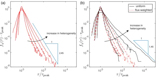
100 102 104 10-8 10-6 10-4 10-2 100 100 102 104 10-8 10-6 10-4 10-2 100 increase in heterogeneity increase in heterogeneity fχ (τ )· τpe ak τ / τpeak τ / τpeak fχ (τ )· τpe ak uniform flux-weighted (b) (a) 1 1.45 1 2.45
Figure 5: (a) FPTDs for σln K = 1, 2, 3, 5 with flux-weighted injection at xc = 200¯l. Increase in conductivity heterogeneity leads to larger dispersion and stronger late-time tailing. (b) FPTDs for σln K = 1, 2, 3, 5 with uniform injection (black solid lines). Uniform injection leads to significantly larger dispersion and late-time tailing compared to the flux-weighted injection (red dashed lines). FPTDs are normalized with the peak arrival time.
Figure 5 shows FPTDs at the outlet, f (τ, xc = 200¯l), for different
con-208
ductivity heterogeneities and injection rules. Conductivity heterogeneity has 209
a clear impact on the FPTD by enhancing longitudinal spreading. This
210
is so because stronger conductivity heterogeneity leads to broader particle 211
transition time distribution, which in turn leads to enhanced longitudinal 212
spreading. The injection rule also has a significant impact on FPTDs espe-213
cially for high conductivity heterogeneity. FPTDs between the two different 214
injection rules are similar for σln K = 1, but uniform injection shows
sig-215
nificantly stronger tailing for σln K = 2, 3, 5 [Figure 5(b)]. As conductivity
216
heterogeneity increases, the flux values at the inlet also becomes broader. 217
For flux-weighted injection, most of particles are injected at the nodes with 218
high flux values. However, for uniform injection, particles are uniformly in-219
jected across the injection nodes and relatively large number of particles are 220
released at the nodes with low flux values. This leads to notable difference 221
between the two injection rules and the difference grows as the conductivity 222
heterogeneity increases. 223
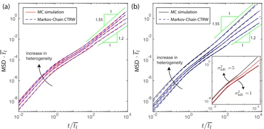
3.2. Centered Mean Square Displacement 224
We also study longitudinal spreading in terms of the centered mean square 225
displacement (cMSD) of average particle density, P (x, t). For the longitudi-226
nal direction (x), the cMSD is given by σ2
x(t) = h[x(t) − hx(t)i]2i where h·i
227
denotes the average over all particles for a given realization. In Figure 6, 228
we show the time evolution of the longitudinal cMSDs. The time axis is 229
normalized with the mean travel time along the characteristic fracture link 230
length, ¯l. For both injection methods, spreading shows a ballistic regime
231
(∼ t2) at early times, which then transitions to a preasymptotic scaling in
an intermediate regime and finally to a final asymptotic regime. The time 233
evolutions of cMSDs for the two injection cases are notably different as con-234
ductivity heterogeneity increases, while the asymptotic late-time scalings are 235
very similar. 236
The asymptotic power-law scaling can be understood in the framework of a continuous time random walk (CTRW) description of dispersion. At large times the Lagrangian velocity distributions are in their steady states and subsequent particle velocities are independent. Thus, at large times horizontal particle dispersion can be described by the CTRW
xn+1 = xn+ `0, tn+1= tn+ τn, (12)
with the transition time τn = `0/vn. The velocities vnare distributed
accord-ing to ps(v) which is space Lagrangian velocity PDF, and `0is a distance along
the streamline that is sufficiently large so that subsequent particle velocities
may be considered independent. Thus, the distribution of transit times τn is
given in terms of the space Lagrangian and Eulerian velocity PDFs as [88]
ψ(τ ) = `0
τ2ps(`0/τ ) =
`0
τ3vpe(`0/τ ), (13)
where v is the average Eulerian velocity, see also Section 4. Specifically, for
the scaling pe(v)∝ vα at small velocities, the transit time PDF scales as
ψ(τ ) ∝ τ−1−β, β = 2 + α. (14)
From Figure 3, we estimate for σln K = 5 that α≈ −0.55, which corresponds
237
to β = 1.45. CTRW theory [66, 65] predicts that the cMSD scales as t3−β,
238
which here implies t1.55. This is consistent with the late-time scaling of the
239
cMSD shown in 6 for σln K = 5.
The Monte Carlo simulations show that, in the intermediate regime (t/tl
241
approximately between 1 and 100), the longitudinal cMSD increases linearly 242
with time for flux-weighted injection [Figure 6(a)]. For uniform injection, 243
cMSD increases faster than linearly (i.e., superdiffusively) for intermediate to 244
strong heterogeneity in the intermediate regime [Figure 6(b)]. The stronger 245
heterogeneity led to the increase in the late-time temporal scaling for both 246
flux-weighted and uniform injection cases. The Monte Carlo simulations also 247
show that there is no noticeable difference between the uniform injection 248
and the flux-weighted injection for the low heterogeneity case whereas the 249
difference increases as heterogeneity increases [Figure 6(b), inset]. 250
In summary, both the increase in conductivity heterogeneity and the uni-251
form injection method enhance longitudinal spreading. For low heterogeneity, 252
the two different injection rules do not affect particle spreading significantly. 253
The difference, however, becomes significant as the conductivity heterogene-254
ity increases. Both the magnitude of the cMSD and the super-diffusive scaling 255
behavior are notably different for the two different injection rules at high het-256
erogeneity. We now analyze the Lagrangian particle statistics to understand 257
the underlying physical mechanisms that lead to the observed anomalous 258
particle spreading. 259
4. Lagrangian Velocity Statistics 260
The classical CTRW approach [64, 65]—see Eq. (12)—relies on the in-261
dependence of particle velocities at subsequent steps and thus spatial po-262
sitions. Recent studies, however, have shown that the underlying mecha-263
nisms of anomalous transport can be quantified through an analysis of the 264
10-2 100 102 104 10-2 100 102 t/ tl t/ tl 10-8 10-6 10-4 10-2 100 10-8 10-6 10-4 10-2 100 · tl · tl MSD MSD (a) (b) MC simulation Markov-Chain CTRW MC simulation Markov-Chain CTRW 104 1.55 1 1.2 1 1.55 1 1.2 1 increase in heterogeneity increase in heterogeneity 10-2 104 10-8 100 σ2 lnK = 1 σ2 lnK = 5
Figure 6: Time evolution of longitudinal MSDs for σln K = 1, 2, 3, 5 obtained from Monte Carlo simulations (solid lines), and the model predictions from the Markov-Chain CTRW (32) and (35) with the full transition PDF (dashed lines). Increase in conductivity het-erogeneity leads to higher dispersion, and the Markov-chain CTRW model is able to accu-rately capture the time evolution of the MSDs for all levels of heterogeneity and injection rules. (a) Flux-weighted injection. (b) Uniform injection. Inset: Comparison between flux-weighted and uniform injection for σln K = 1, 5. Impact of injection rule is significant for high conductivity heterogeneity.
statistics of Lagrangian particle velocities such as velocity distribution and 265
correlation [74, 76, 98, 77, 78, 45, 80]. In the following, we briefly intro-266
duce two viewpoints for analyzing Lagrangian velocities—equidistantly and 267
isochronally along streamlines—and the relation between them [88]. We then 268
proceed to a detailed analysis of the Lagrangian velocity statistics measured 269
equidistantly along streamlines. 270
4.1. Lagrangian Velocities 271
Particle motion is described here by the recursion relations (7). In this
framework, we consider two types of Lagrangian velocities. The t(ime)–
Lagrangian velocities are measured at a given time t,
vt(t) = unt, (15)
where nt is defined by (8). The s(pace)–Lagrangian velocities are measured
at a given distance s along the trajectory. The distance sn traveled by a
particle along a trajectory after n steps is given by
sn+1 = sn+ `n. (16)
The number of steps needed to cover the distance s is described by ns =
sup(n|sn ≤ s). Thus, the particle velocity at a distance s along a trajectory
is given by
vs(s) = uns. (17)
The PDF of t–Lagrangian velocities sampled along a particle path is given by pt(v) = lim n→∞ Pn i=1τiδ(v− ui) Pn i=1τi , (18)
where we defined the transit time, τi =
`i
ui
(19) The PDF of s–Lagrangian velocities sampled along a particle path are defined analogously as ps(v) = lim n→∞ Pn i=1`iδ(v− ui) Pn i=1`i . (20)
Note the difference with respect to Eq. (2), which samples velocities in the network uniformly, while in Eq. 20 velocities are sampled along trajectories.
Using the definition of the transit time τi in (19), the PDFs of the s– and
t–Lagrangian velocities are related through flux weighting as [88] ps(v) =
vpt(v)
Z
dv vpt(v)
. (21)
Furthermore, for flux-preserving flows and under ergodic conditions, the Eu-lerian and t-Lagrangian velocity PDFs are equal,
pe(v) = pt(v). (22)
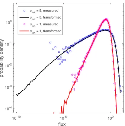
Thus, under these conditions, the s–Lagrangian and Eulerian velocity PDFs are related as [88] ps(v) = vpe(v) Z dv vpe(v) . (23)
This means that the stationary s-Lagrangian velocity PDF can be determined 272
from the Eulerian velocity PDF. Figure 7 illustrates this relation by compar-273
ing the s-Lagrangian velocity PDFs measured from the numerical simulation 274
to the flux-weighted Eulerian velocity PDFs shown in Figure 3. 275
flux 10-10 10-5 100 probability density 10-4 10-3 10-2 10-1 100 σlnK = 5, measured σlnK = 5, transformed σlnK = 1, measured σlnK = 1, transformed
Figure 7: s-Lagrangian velocity PDFs for σlnK = 1 and σlnK = 5. The measured s-Lagrangian velocity PDF agrees very well with the PDF obtained by transforming the Eulerian velocity PDF using Eq. (23).
4.2. Evolution of Lagrangian Velocity Distributions 276
It is important to emphasize that the above definitions of the Lagrangian velocity PDFs refer to stationary conditions. We now define the PDFs of t– and s–Lagrangian velocities through sampling between particles and network realizations at a given time (t-Lagrangian) or space (s-Lagrangian) velocities
ˆ
pt(v, t) =hδ[v − v(t)]i, pˆs(v, s) =hδ[v − v(s)]i. (24)
In general, these quantities evolve in time and with distance along the stream-line and are sensitive to the injection conditions because evidently for t = 0
and s = 0 both are equal to the PDF of initial particle velocities ˆpt(v, t =
0) = ˆps(v, s = 0) = p0(v), but their respective stationary PDFs are different,
namely
pt(v) = lim
t→∞pˆt(v, t), ps(v) = lims→∞pˆs(v, s). (25)
Let us consider some further consequences of these properties. First, we notice that under (Eulerian) ergodicity the uniform injection condition (4) corresponds to an initial velocity PDF of
p0(v) = pe(v) = pt(v), (26)
that is, the initial velocity PDF is equal to the Eulerian and thus t–Lagrangian 277
velocity PDFs. This means that for the uniform injection method, the t– 278
Lagrangian velocity PDF is steady, ˆpt(v, t) = pt(v), while the s–Lagrangian
279
velocity PDF is not. It evolves from its initial distribution ps(v, s = 0) =
280
pe(v) to the steady state distribution (23).
The flux-weighted injection condition, on the other hand, corresponds to the the initial velocity PDF
p0(v) = ps(v), (27)
due to relation (21). The initial velocity PDF is equal to the s–Lagrangian 282
velocity PDF. This means that under flux-weighting, the s–velocity PDF is 283
steady, ˆps(v, s) = ps(v). Under these conditions, the t–Lagrangian velocity
284
PDF ˆpt(v, t) evolves from the initial distribution ˆpt(v, t = 0) = ps(v) towards
285
the asymptotic pt(v) = pe(v), which is equal to the Eulerian velocity PDF.
286
These are key insights for the qualitative and quantitative understanding of 287
the average transport behavior. 288
4.3. Space-Lagrangian Velocity Statistics 289
We analyze particle velocities along their projected trajectories in the 290
longitudinal direction. Spatial particle transitions may be characterized by 291
the characteristic fracture link length, ¯l. The Lagrangian velocity vs(sn) at
292
a distance xn = n¯l along the projected trajectory is approximated by the
293
average velocity vn ≡ ¯l/τn where τn is the transition time for the distance
294 ¯
l at step n. In the following, we investigate the statistical characteristics of 295
the s-Lagrangian velocity series {vn}. For the uniform flow conditions under
296
consideration here, the projected distance xnis a measure for the streamwise
297
distance sn, and vn for the s-Lagrangian velocity vs(sn). Spatial Lagrangian
298
velocities have been studied by Cvetkovic et al. [73] and Gotovac et al. [75] 299
for highly heterogeneous porous media and by Frampton and Cvetkovic [16] 300
for 3D DFNs in view of quantifying particle travel time statistics and thus 301
modelling effective particle motion. 302
normalized flux 10-10 10-8 10-6 10-4 10-2 100 probability density 10-3 10-2 10-1 100 101 102 103 104 105 106 uniform - inlet uniform - outlet flux - inlet flux - outlet normalized flux 10-10 10-5 100 probability density 10-2 100 102 104 106
Figure 8: Lagrangian flux distributions at the inlet and outlet for uniform and flux-weighted injection rules, for σlnK = 5. Note that Lagrangian flux distributions at the outlet are identical regardless of the injection method. Inset: the same plot for σlnK = 1.
We first study the convergence of the s–Lagrangian velocity PDFs towards 303
a stationary distribution and the invariance of ˆps(v, s) for a stationary
(flux-304
weighted) initial velocity PDF. We consider the two injection conditions (4) 305
and (5) and record the distribution of particle velocities at a line located at 306
the control point xc. Under ergodic conditions, we expect ˆps(v, s) to converge
307
towards its steady state distribution (23) for uniform injection and to remain 308
invariant for the flux-weighted injection. Figure 8 shows ˆps(v, s = 0) and
309
ˆ
ps(v, s = xc) for uniform and flux-weighted injection conditions and two
310
different heterogeneity strengths. We clearly observe that ˆps(v, xc) = ps(v)
311
is invariant for flux-weighted injection. For uniform injection, ˆps(v, xc) has
312
already evolved towards its steady limit after xc = 200¯l. This is an indication
313
that the flow and transport system is in fact ergodic. Note that in terms 314
of computational efficiency, this observation gives a statistically consistent 315
way of continuing particle trajectories through reinjection at the inlet. If 316
the outlet is located at a position xc large enough so that ˆps(v, s = xc) =
317
ps(v), particles are reinjected at the inlet with flux-weighted probability, this
318
means that the velocity statistics are preserved. Furthermore, this method 319
ensures that the domain is large enough to provide ergodic conditions. In 320
the following, we analyze the statistical properties of streamwise velocity 321
transitions with the aim of casting these dynamics in the frame of a Markov 322
model for subsequent particle velocities. 323
We first consider the distribution ψτ(t) of transition times along particle
324
trajectories through sampling the transition times along all particle trajecto-325
ries and among network realizations. To this end, we consider a flux-weighted 326
injection because it guarantees that the s-Lagranagian velocities are station-327
ary. Figure 9 illustrates the PDF of transition times for different variances 328
of ln(K). As σln K increases, the transition time PDFs become broader. The
329
transition time closely follows a truncated power-law distribution. 330
Next we consider two-point velocity statistics to gain insight into the velocity correlations along a streamline. To this end, we consider the velocity
auto covariance for a given lag ∆s = s− s0. As pointed out above, for
flux-weighted injection, the streamwise velocities here are stationary and therefore Cs(s− s0) = h[vs(s)− hvs(s)i][vs(s0)− hvs(s0)i]i. (28)
In order to increase the statistics, we furthermore sample along streamlines
over a distance of 102¯l. The velocity variance is σ2v = Cs(0). The velocity
autocorrelation function χs(s) = Cs(s)/σ2v. The correlation length scale `cis
defined by `c= ∞ Z 0 ds χs(s). (29)
The inset in Figure 9 shows the increase in the velocity correlation length 331
scale with increasing ln(K) variances for a flux-weighted injection case. This 332
can be attributed to the emergence of preferential flow paths, as shown in 333
Figure 2. Painter and Cvetkovic [71] and Frampton and Cvetkovic [16] also 334
reported the existence of clear velocity correlation between successive jumps 335
in DFNs and showed that this correlation structure should be captured for 336
effective transport modelling. 337
The existence of a finite correlation length along the particle trajectories indicates that subsequent velocities, when sampled at a distance much larger
10-2 100 102 104 106 10-12 10-8 10-4 100 σlnK=1 σlnK=2 σlnK=3 σlnK=5 ψτ (t )· tl t/ tl 1 1 2.45 2.85 σ2lnK 1 2 3 4 5 n c 3 5 7 9 11
Figure 9: (a) Lagrangian transition time distributions for σln K = 1, 2, 3, 5 with flux-weighted injection. As the network conductivity becomes more heterogeneous, the tran-sition time distribution becomes broader. Inset: the effective correlation length increases with increasing network heterogeneity: 3.8¯l, 5.6¯l, 8.2¯l, 11.5¯l. The correlation step (nc) is computed by integrating velocity autocorrelation function in space.
study this feature, we characterize the series of s-Lagrangian velocities {vn}
in terms of the transition probabilities to go from velocity vm to velocity
vm+n. We determine the transition probabilities under flux-weighted particle
injection because, as detailed above, under these conditions, the s-Lagrangian velocity is stationary. Thus, the transition probability is only a function of the number n of steps,
rn(v|v0) = hδ(v − vm+n)i |vm=v0 (30)
Numerically, the transition probability is determined by discretizing the
s-Lagrangian velocity PDF into N velocity classes Ci = (vs,i, vs,i+ ∆vs,i) and
recording the probability for each class given the previous velocity class. This
procedure gives the transition matrix Tn(i|j) from class j to i after n steps
such that rn(v|v0) is approximated numerically as
rn(v|v0) = N X i,j=1 ICi(v)Tn(i|j)ICj(v 0) ∆vi , (31)
where the indicator function ICi(v) is 1 if v∈ Ci and 0 otherwise.
338
Figure 10 shows the one-step transition matrix T1(i|j) for equidistant and
339
logarithmically equidistant velocity classes for different network heterogene-340
ity. Higher probabilities along the diagonal than in the off-diagonal positions 341
indicate correlation between subsequent steps, which, however, decreases as 342
the number of steps along the particle trajectory increases, as indicated by 343
the existence of a finite correlation scale `c.
344
5. Stochastic Particle Motion and Effective Transport Model 345
In the following, we describe the evolution of the s-Lagrangian velocities 346
by a Markov-chain, which is motivated by the existence of a finite spatial 347
(a) (b)
(c) (d)
current velocity class
current velocity class
current velocity class
ne xt v elocit y class ne xt v elocit y class ne xt v elocit y class -6 -5 -4 -3 -2 -6 -5 -4 -3 -2
current velocity class
ne
xt v
elocit
y class
Figure 10: (a) One-step velocity transition matrix T1(i|j) with linear equiprobable binning for N = 50 velocity classes for σln K = 1. (b) Velocity transition matrix with linear equiprobable binning for σln K = 5. The color-bar shows the logarithmic scale. (c) Velocity transition matrix with logarithmic binning for σln K = 1. (d) Velocity transition matrix with logarithmic binning for σln K = 5. Increase in conductivity heterogeneity leads to higher probability close to diagonal entries.
correlation scale (see inset of figure 9). This leads to a spatial Markov-chain 348
random walk (which we also termed spatial Markov Model) formulation of 349
particle dispersion that is valid for any initial velocity distribution, and thus 350
for any injection protocol. This modelling approach is in line with the time-351
domain random walk (TDRW) and continuous time random walk (CTRW) 352
approaches discussed in the Introduction and below. 353
5.1. Markovian Velocity Process 354
Along the lines of Le Borgne et al. [74] and Kang et al. [77], we model
the velocity series {vn} as a Markov-chain, which is a suitable model to
sta-tistically quantify the evolution of the s-Lagrangian velocities based on the existence of a finite correlation length. In this framework, the n–step
tran-sition probability rn(v|v0) satisfies the Chapman–Kolmogorov equation [99]
rn(vn|v0) =
Z
dvkrn−k(vn|vk)rk(vk|v0). (32a)
The velocity process is fully characterized in terms of the one-step transition
PDF r1(v|v0) and the steady state PDF ps(v) of the s-Lagrangian velocity.
Consequently, the evolution of the s-Lagrangian velocity PDF ˆps(v, sn) is
given by
ps(v, sn) =
Z
dv0r1(v|v0)ps(v0, sn), (32b)
with the arbitrary initial PDF ps(v, s0 = 0) = p0(v). The number of steps
355
to decorrelate this Markov-chain is given by nc = `c/¯l. Figure 11 shows the
356
evolution of the PDF of s-Lagrangian velocities for the uniform injection (4). 357
Recall that the uniform injection mode corresponds to the initial velocity 358
PDF pe(v). Thus, the numerical Monte Carlo simulations are compared to
359
the predictions of (32b) for the initial condition ˆps(v, s0 = 0) = pe(v). The
360
transition PDF r1(v|v0) is given by (31) with the velocity transition matrix
361
shown in Figure 10. As shown in Figure 11, the prediction of the Markovian 362
velocity model and the Monte Carlo simulation are in excellent agreement, 363
which confirms the validity of the Markov model (32) for the evolution of 364
s-Lagrangian velocities. Velocity transition dynamics are independent of the 365
particular initial conditions and thus allow predicting the evolution of the 366
Lagrangian velocity statistics for any initial velocity PDF and thus for any 367
injection protocol. 368
As mentioned above, the Markov-chain {vn} is fully characterized by
the stationary PDF of the s-Lagrangian velocities and the transition PDF
r1(v|v0). The behavior of the latter may be characterized by the number of
steps nc needed to decorrelate, i.e., the number of steps ncsuch that rn(v|v0)
for n > nc converges to the stationary PDF rn(v|v0) → ps(s). The number
of steps for velocities to decorrelate can be quantified by
nc=
`c
¯l , (33)
The simplest transition PDF that shares these characteristics is [41, 80, 50, 88]
r1(v|v0) = aδ(v− v0) + (1− a)ps(v), (34)
with a = exp(−¯l/`c). This transition PDF is thus fully determined by one
369
single parameter nc. Note that the latter increases with the level of
hetero-370
geneity, as illustrated in the inset of figure 9. This parameter is estimated 371
here from the simulated Lagrangian velocities. It may also be measured in 372
the field from multiscale tracer tests [41]. In the following, we study particle 373
dispersion in the Markovian velocity model for the full transition PDF shown 374
in Figure 10 and the reduced-order Markov model (34). 375
5.2. Particle Dispersion and Model Predictions 376
We consider particle motion along the mean pressure gradient in x– direction, which is described by the stochastic regression
xn+1 = xn+ ¯l, tn+1= tn+
¯ l vn
. (35)
The velocity transitions are determined from the Markovian velocity
pro-cess (32). Note that the {vn} process describes equidistant velocity
tran-sitions along particle trajectories, while (35) describes particle motion pro-jected on the x-axis. In this sense, (35) approximates the longitudinal travel
distance xn with the distance sn along the streamline, which is valid if the
tortuosity of the particle trajectories is low. As indicated in Section 3.2, for
travel distances `0 larger than `c, or equivalently, step numbers n nc ≡
`c/¯l, subsequent velocities may be considered independent and particle
dis-persion is fully characterized by the recursion relation (12) and the transition time PDF (13). Thus, as shown in Section 3.2, the CTRW of Eq. (12) cor-rectly predicts the asymptotic scaling behavior of the centered mean square displacement. This is not necessarily so for the particle breakthrough and the preasymptotic behavior of the cMSD. As seen in Section 3.1, the late time tailing of the BTC depends on the injection mode and thus on the initial velocity PDF. In fact, the slope observed in Figure 5 for uniform particle in-jection can be understood through the persistence of the initial velocity PDF.
flux 10-10 10-8 10-6 10-4 10-2 100 probability density 10-2 100 102 104 106 at at at at CTRW prediction 10-5 10-3 10-1 101 10-3 10-2 10-1 100 at at CTRW prediction 5¯l 50¯l 50¯l 10¯l 5¯l ¯l
Figure 11: Evolution of the PDF of s-Lagrangian velocities for uniform injection, i.e., for an initial velocity PDF ˆps(v, s0 = 0) = pe(v). The symbols denote the data obtained from the direct numerical simulation, the dashed lines show the predictions of (32b) with the transition matrix shown in Figure 10. Inset: Evolution of the PDF of s-Lagrangian velocities for a flux-weighted injection. In this case, the initial velocity PDF is identical to the stationary s-Lagrangian velocity PDF.
by the transit time PDF
ψ0(t) =
¯ l
t2p0(¯l/t). (36)
Thus, for an initial velocity PDF p0(v) = pe(v), the initial transit time PDF
is given in terms of the Eulerian velocity PDF, which is characterized by a stronger probability weight towards low velocities than the PDF of the
s-Lagrangian velocities, which is given by (23). The space-time random
walk (35) together with the Markov model (32b) is very similar to the TDRW approach [70, 71] and can also be seen as a multi-state, or correlated CTRW approach because subsequent particle velocities and thus transition times are represented by a Markov process [100, 101, 74, 102]. The joint distribution p(x, v, t) of particle position and velocity at a given time t is given by [74]
p(x, v, t) =
t
Z
0
dt0H(¯l/v− t0)R(x− vt0, v, t− t0), (37)
where H(t) is the Heaviside step function; R(x, v, t) is the frequency by which a particle arrives at the phase space position (x, v, t). It satisfies
R(x, v, t) = R0(x, v, t) +
Z
dv0r1(v|v0)R(x− ¯l, v0, t− ¯l/v0), (38)
where R0(x, v, t) = p0(x, v)δ(t) with p0(x, v) = p(x, v, t = 0). Thus, the right
side of (37) denotes the probability that a particle arrives at a position x−vt0
where it assumes the velocity v by which it advances toward the sampling position x. Equations (37) and (38) can be combined into the Boltzmann equation ∂p(x, v, t) ∂t =−v ∂p(x, v, t) ∂x − v ¯ lp(x, v, t) + Z dv0v 0 ¯ l r1(v|v 0)p(x, v0, t), (39)
see Appendix A. This result provides a bridge between the TDRW ap-377
proach [70, 71] and the correlated CTRW approach. 378
As illustrated in Figure 3, the Eulerian velocity PDF can be characterized 379
by the power-law pe(v) ∝ vα. Thus, the first CTRW steps until the
decor-380
relation at n = nc are characterized by the transit time PDF ψ0(t)∝ t−2−α.
381
The corresponding tail of the BTC is f (t, xc) ∝ t−2−α. The observed value
382
of α = −0.55 explains the tailing of the BTC in Figure 5 as t−1.45, which
383
shows the importance of the initial velocity distribution. We also observe 384
decrease in BTC tailing (larger absolute slope) with travel distance as initial 385
velocity distribution converges to stationary Lagrangian velocity distribution 386
and as tracers sample more velocity values. This implies that one needs to be 387
careful when inferring a β from single BTC measurement because the slope 388
can evolve depending on the injection method, velocity PDF and velocity 389
correlation. 390
First, we compare the results obtained from Monte Carlo simulation in 391
the random DFN to the predictions of the Markov-chain CTRW (32) and 392
(35) with the full transition PDF of Figure 10. Figure 6 shows the evolu-393
tion of the cMSD for different levels of heterogeneity and different injection 394
modes. As expected from the ability of the Markov model to reproduce 395
the evolution of the s-Lagrangian velocity PDF for both uniform and flux-396
weighted injection conditions, the predictions of particle spreading are in 397
excellent agreement with the direct numerical simulations. In Figure 12 we 398
compare breakthrough curves obtained from numerical simulations with the 399
predictions by the Markov model for the uniform and flux-weighted injection 400
modes. Again, the impact of the injection mode and thus initial velocity 401
PDF is fully quantified by the Markov model. 402
We now apply the Markov model (32)–(35), i.e., employing a parsimo-403
nious parameterization of the velocity transition PDF, with a single param-404
eter nc (equation (33)), which is estimated here from velocity correlations
405
along streamlines (see inset of figure 9). We first compare the reduced-order 406
Markov model to the cases of uniform and flux-weighted injection, and con-407
clude that the proposed parsimonious stochastic model provides an excellent 408
agreement with the direct numerical simulations (Figure 13). This implies 409
that the simple correlation model (34) can successfully approximate the ve-410
locity correlation structure. Hence it appears that high order correlation 411
properties, quantified from the full transition probabilities (figure 10), are 412
not needed for accurate transport predictions in the present case. This sug-413
gests promising perspective for deriving approximate analytical solutions for 414
this Markov-chain CTRW model [88]. Furthermore, as discussed in [41], the 415
velocity correlation parameter nc can be estimated in the field by combining
416
cross-borehole and push-pull tracer experiments. 417
Finally, we consider the evolution of the particle BTC and the cMSD for 418
arbitrary injection modes. For real systems both flux-weighted and uniform 419
injections are idealizations. A flux-weighted condition simulates a constant 420
concentration pulse where the injected mass is proportional to the local in-421
jection flux at an inlet boundary that is extended over a distance much larger 422
than the correlation scale during a given period of time. A uniform injection 423
represents an initial concentration distribution that is uniformly extended 424
over a region far larger than the correlation length. In general, the initial 425
concentration distribution may not be uniform, and the injection boundary 426
may not be sufficiently large, which leads to an arbitrary initial velocity dis-427
tribution, biased maybe to low or high flux zones, as for example in the 428
MADE experiments, where the solute injection occurred into a low perme-429
ability zone [103]. For demonstration, we study two scenarios representing 430
injection into low and high flux zones: uniform injections into regions of the 431
20-percentile highest, and 20-percentile lowest velocities. The initial velocity 432
PDF for the low velocity mode shows the power-law behavior which is the 433
characteristic for the Eulerian PDF, and the initial velocity PDF for the high 434
velocity mode shows narrow initial velocity distribution (Figure 15). Even-435
tually, the s-Lagrangian PDFs evolve towards the stationary flux-weighted 436
Eulerian PDF as discussed in the previous section. 437
Figure 15 shows the predictive ability of the effective stochastic model 438
for these different injection conditions. The reduced-order Markov velocity 439
model compares well with the direct Monte Carlo simulation in the random 440
networks. As expected, the BTCs for injection into low velocity regions 441
have a much stronger tailing than for injection into high velocity regions. 442
In fact, as the initial velocity shows the same behavior at low velocities as 443
the Eulerian velocity PDF, the breakthrough tailing is the same as observed 444
in Figure (12). We also observed that the reduced-order Markov velocity 445
model can capture important features of the time evolution of cMSDs. This 446
demonstrates that the proposed model can incorporate arbitrary injection 447
modes into the effective modelling framework. 448
100 102 104 10-8 10-6 10-4 10-2 100 1 2.45 100 102 104 10-8 10-6 10-4 10-2 100 1 1.45 fχ (τ ) τ τ fχ (τ ) (b) (a) MC simulation Correlated CTRW MC simulation Correlated CTRW
Figure 12: Particle BTCs from Monte Carlo simulations and the predictions from the Markov-chain CTRW model with the full velocity transition matrix for (a) flux-weighted injection, and (b) uniform injection at xc = 200¯l.
100 102 104 10-8 10-6 10-4 10-2 100 100 102 104 10-8 10-6 10-4 10-2 100 fχ (τ ) τ τ fχ (τ ) (b) (a) MC simulation Correlated CTRW MC simulation Correlated CTRW 1 2.45 1 1.45
Figure 13: Particle BTCs from Monte Carlo simulations and predictions from the Markov-chain CTRW model with the reduced-order velocity transition matrix for (a) flux-weighted injection, and (b) uniform injection at xc = 200¯l.
normalized flux 10-10 10-8 10-6 10-4 10-2 100 probability density 10-3 10-2 10-1 100 101 102 103 104 105 106 low - inlet low - outlet high - inlet high - outlet normalized flux 10-10 100 probability density 10-2 106
Figure 14: Lagrangian flux distributions at the inlet and outlet with two arbitrary initial velocity distributions for σln K = 5. The two initial velocity distributions come from uni-form injections into regions of the 20-percentile highest, and 20-percentile lowest velocities. Flux values are normalized with the mean flux value. Note that flux distributions at outlet are identical regardless of the initial velocity distribution. Inset: same plot for σln K = 1.
100 102 104 10-8 10-6 10-4 10-2 100 100 102 104 10-8 10-6 10-4 10-2 100 fχ (τ ) τ τ fχ (τ ) (b) (a) MC simulation Correlated CTRW MC simulation Correlated CTRW 1 2.45 1 1.45
Figure 15: (a) Particle BTCs from Monte Carlo simulations for injection into high-velocity regions (solid line) and predictions from Markov-chain CTRW model with the reduced-order velocity transition matrix (dashed line). (b) Corresponding results for injection into low-velocity regions.
6. Conclusions 449
This study shows how the interplay between fracture geometrical prop-450
erties (conductivity distribution and network geometry) and tracer injection 451
modes controls average particle transport via Lagrangian velocity statistics. 452
The interplay between fracture heterogeneity and tracer injection methods 453
can lead to distinctive anomalous transport behavior. Furthermore, the in-454
jection conditions, for example, uniform or flux-weighted, imply different 455
initial velocity distributions, which can have a persistent impact on particle 456
spreading through DFNs. For uniform injection, the s-Lagrangian velocity 457
distribution evolves from an Eulerian velocity distribution initially to a sta-458
tionary s-Lagrangian distribution. In contrast, for flux-weighted injection, 459
the s-Lagrangian velocity distribution remains stationary. 460
We have presented a spatial Markov model to quantify anomalous trans-461
port through DFNs under arbitrary injection conditions. We derive an ana-462
lytical relation between the stationary Lagrangian and the Eulerian velocity 463
distribution, and formally incorporate the initial velocity distribution into the 464
spatial Markov model. The proposed model accurately reproduces the evo-465
lution of the Lagrangian velocity distribution for arbitrary injection modes. 466
This is accomplished with a reduced-order stochastic relaxation model that 467
captures the velocity transition with a single parameter: the effective ve-468
locity correlation `c. The agreement between model predictions and direct
469
numerical simulations indicates that the simple velocity correlation model 470
can capture the dominant velocity correlation structure in DFNs. 471
In this study, we investigated the particle transport and the impact of 472
the injection condition for idealized 2D DFN using a Markov velocity model. 473
These findings can be extended to 3D DFNs, for which similar behaviors 474
regarding the injection mode have been found [58]. Also, Frampton and 475
Cvetkovic [16] reported similar velocity correlation structures for 3D DFNs 476
as in 2D, which suggests that a velocity Markov model such as the one 477
presented in this work can be used for the modelling of particle motion in 478
3D DFNs. 479
Acknowledgements: PKK and SL acknowledge a grant (16AWMP-480
B066761-04) from the AWMP Program funded by the Ministry of Land, 481
Infrastructure and Transport of the Korean government and the support 482
from Future Research Program (2E27030) funded by the Korea Institute of 483
Science and Technology (KIST). PKK and RJ acknowledge a MISTI Global 484
Seed Funds award. MD acknowledges the support of the European Research 485
Council (ERC) through the project MHetScale (617511). TLB acknowledges 486
the support of European Research Council (ERC) through the project Re-487
activeFronts (648377). RJ acknowledges the support of the US Department 488
of Energy through a DOE Early Career Award (grant DE-SC0009286). The 489
data to reproduce the work can be obtained from the corresponding author. 490
Appendix A. Boltzmann Equation 491
The time derivative of (37) gives ∂p(x, v, t)
∂t =−v
∂p(x, v, t)
∂x + R(x, v, t)− R(x − ¯l, v, t − ¯l/v). (A.1)
Note that R(x, v, t) denotes the probability per time that a particle has the velocity v at the position x. It varies on a time scale of ¯v. Thus we can approximate (37) as
p(x, v, t)≈
¯l
vR(x− ¯l, v, t − ¯l/v). (A.2)
Using this approximation and combining (A.1) with (38) gives for t > 0 ∂p(x, v, t) ∂t =−v ∂p(x, v, t) ∂x − v ¯ lp(x, v, t) + Z dv0r1(v|v0) v0 ¯ l p(x, v 0 , t). (A.3) 492 References 493
[1] G. S. Bodvarsson, W. B., R. Patterson, D. Williams, Overview of sci-494
entific investigations at Yucca Mountain: the potential repository for 495
high-level nuclear waste, J. Contaminant Hydrol. 38 (1999) 3–24. 496
[2] J. L. Lewicki, J. Birkholzer, C. F. Tsang, Natural and industrial ana-497
logues for leakage of CO2 from storage reservoirs: identification of fea-498
tures, events, and processes and lessons learned, Environ. Geol. 52 (3) 499
(2007) 457–467. 500
[3] D. H. Tang, E. O. Frind, E. A. Sudicky, Contaminant transport in 501
fractured porous media: Analytical solution for a single fracture, Water 502
Resour. Res. 17 (3) (1981) 555–564. 503
[4] C. V. Chrysikopoulos, C. Masciopinto, R. La Mantia, I. D. Manariotis, 504
Removal of biocolloids suspended in reclaimed wastewater by injection 505
into a fractured aquifer model, Environ. Sci. Technol. 44 (3) (2009) 506
971–977. 507
[5] K. Pruess, Enhanced geothermal systems (EGS) using CO2 as working
508
fluid: novel approach for generating renewable energy with simultane-509
ous sequestration of carbon, Geothermics 35 (2006) 351–367. 510
[6] S. P. Neuman, C. L. Winter, C. M. Newman, Stochastic theory of field-511
scale Fickian dispersion in anisotropic porous media, Water Resour. 512
Res. 23 (3) (1987) 453–466. 513
[7] Y. W. Tsang, C. F. Tsang, F. V. Hale, B. Dverstorp, Tracer transport 514
in a stochastic continuum model of fractured media, Water Resour. 515
Res. 32 (10) (1996) 3077–3092. 516
[8] L. Kiraly, Remarques sur la simulation des failles et du r´eseau
kars-517
tique par ´el´ements finis dans les mod`eles d’´ecoulement, Bull. Centre
518
Hydrog´eol. 3 (1979) 155–167, Univ. of Neuchˆatel, Switzerland.
[9] M. C. Cacas, E. Ledoux, G. de Marsily, B. Tillie, A. Barbreau, E. Du-520
rand, B. Feuga, P. Peaudecerf, Modeling fracture flow with a stochas-521
tic discrete fracture network: Calibration and validation: 1. The flow 522
model, Water Resour. Res. 26 (3) (1990) 479–489. 523
[10] A. W. Nordqvist, Y. W. Tsang, C. F. Tsang, B. Dverstorp, J. Anders-524
son, A variable aperture fracture network model for flow and transport 525
in fractured rocks, Water Resour. Res. 28 (6) (1992) 1703–1713. 526
[11] L. Moreno, I. Neretnieks, Fluid flow and solute transport in a network 527
of channels, J. Contaminant Hydrol. 14 (1993) 163–194. 528
[12] R. Juanes, J. Samper, J. Molinero, A general and efficient formulation 529
of fractures and boundary conditions in the finite element method, Int. 530
J. Numer. Meth. Engrg. 54 (12) (2002) 1751–1774. 531
[13] Y. J. Park, K. K. Lee, G. Kosakowski, B. Berkowitz, Transport be-532
havior in three-dimensional fracture intersections, Water Resour. Res. 533
39 (8) (2003) 1215. 534
[14] M. Karimi-Fard, L. J. Durlofsky, K. Aziz, An efficient discrete fracture 535
model applicable for general purpose reservoir simulators, Soc. Pet. 536
Eng. J. 9 (2) (2004) 227–236. 537
[15] L. Martinez-Landa, J. Carrera, An analysis of hydraulic conductiv-538
ity scale effects in granite (Full-scale Engineered Barrier Experiment 539
(FEBEX), Grimsel, Switzerland), Water Resour. Res. 41 (3) (2005) 540
W03006. 541