An approach to parameter sensitivity analyses in model assessment

ANALYSES IN MODEL ASSESSMENT

by

Cecilia Sau Yen Wong

June 1978

MIT Energy Laboratory

ACKNOWLEDGEMENTS

This research was conducted as part of the M.I.T. Energy Laboratory's Model Assessment Project with support from the Electric Power Research

Institute. The author expresses her deep gratitude to Professor Fred Schweppe for his advice and help in preparing this paper.

Page

1. Introduction 4

2. Static Generation Expansion 7

2.1 No Existing Systems ₁₁

2.2 Existing Systems ₂₀

2.3 Generalizing the Results ₂₅

3. Criteria Sensitivity ₂₈

4. Application to REM ₃₂

5. Discussion and Extensions ₄₆

Section 1: INTRODUCTION

The effect of parameter variation on system performance is important in system analysis and especially important for model assessment. The technique of parameter sensitivity analysis as, for example, that

introduced into feedback system by Bode (1) and extended by Horowitz (2) is a measure of the change in some desired quantity with respect to the change in some system parameters(3). If T is the desired quantity and is the parameter, the sensitivity function is given by

T T a

a

,

'

T.

Cruz (4), Perkins (5), and Morgans (6) have done extended work on linear multivariable systems.

Although such sensitivities are appropriate when taken in the

context in which one intended, they are inadequate for model assessment. Parameter sensitivity analysis for model assessment should adopt an approach similar to that of building a model. The complexity of the model structure depends on the purposes of building the model.

Similarly, the sensitivity of a model should depend on the criteria set for analyzing that model. It would be more appropriate to predetermine a sequence of criteria and then obtain the parameter sensitivity with

respect to each criterion. A model could well be sensitive to one criterion and very insensitive to another. Rather than using the usual definitions of sensitivity, a new approach on parameter sensitivity is introduced for model assessment. This approach, named criteria

sensitivity, is represented by the relationship between the percentage change in parameter vector and the minimum value of the performance

indicator* of a criterion. The main idea is to present the sensitivity in two-dimensional space; one axis represents the minimum value of the performance indicator of a criterion, and the other axis represents the percentage change in parameter vector at its nominal value. Knowing the relationship between the minimum value and the percentage change, one would get a good picture of how sensitive the model criterion is with respect to parameter change.

This report uses the above sensitivity analysis on

1. the logic of optimal plant mixes to illustrate such a new approach, and

2. the generation expansion submodel of the Regional Electricity Model, REM (7), as an example for applying such an approach to dynamic systems in general.

This report is organized as follows. Section 2 considers the static generation expansion problem (i.e., fixed year, no time dynamics). The numerical results and discussion of this static problem act as a vehicle to explain the basic ideas of this sensitivity analysis. The ideas of Section 2 are then abstracted and generalized in Section 3 to yield a more complete concept with an application to arbitrary dynamic systems. In Section 4, these general ideas are applied to the REM** study, which

*Criterion is used as a verbal description of rules for judging the effect of parameter changes on some concerns. These concerns are

represented mathematically by the performance indicator which is a scalar function.

**It is assumed that the reader is already familar with generation expansion logic in general and REM in particular.

is a dynamic model. Finally, the extension of the new theory and the relationship between parameter sensitivity and model validity are discussed in Section 5.

Section 2: STATIC GENERATION EXPANSION

For the purpose of illustrating this new approach to sensitivity analysis, let us analyze the static optimal plan mix logic by Turvey (8) for a particular region at time, say, 1975. The logic of optimal plant mix in electricity supply is to choose the plant composition for

minimizing the average cost per kilowatt hour. The principal economic parameters of this cost are capital costs, operation and maintenance costs, fuel costs, and heat rates. The average cost equation defined in REM (9) is

cost -= Pa + Pb

usage (mills/kWh)

Pa = CHRATE * (PCAPIT + CFULK2) the usage-dependent 8.76 * AVAFAC * DUTMAX ge-dependent

component of production cost,

Pb = CFULM2 + POAMCO, the usage-independent component of production cost, where

CHRATE = capital charge rate for planning

PCAPIT = predicted capital cost for plant type j CFULK2 = cost of nuclear fuel loading

AVAFAC = availability factor

DUTMAX = maximum allowable duty cycle

CFULM2 = predicated fossil fuel cost for plant type j POAMCO = predicated O&M cost for plant type j.

Assume there are six plant alternatives: coal-fired thermal, oil-fired thermal, light water uranium reactors; light water plutonium reactors, high-temperature gas reactors, and liquid metal fast breeder reactors. The optimal mix is to find a plant composition with minimum cost. Assume the parameter values are as given in Table 1. The optimal plan mix is OIL, COAL, and LWRU as indicated in Figure 1.

Table 1

NOMINAL VALUES OF PARAMETERS

PLANT COAL OIL LWR LWR HTGR LMFBR

PARAMETER U-235 PU-U

CHRATE .1487 .1487 .1487 .1487 .1487 .1487 PCAPIT ($/kW) 391.3 351.6 456.1 683.1 746.0 909.5 CFULK2 ($/kW) 0 0 45.61 456.10 5.21 38.97 AVAFAC .85 .95 .85 .70 .70 .70 DUMAX .9 .9 .86 .86 .86 .86 Pa (mills/kWh) 8.680 6.979 11.650 32.110 21.180 26.74 CFULM2 11.09 17.14 3.131 31.31 2.244 -.3466 (mills/kWh) POAMCO .4797 .4797 .6396 .6396 .6396 .6396 (mills/kWh) Pb 11.57 17.62 3.771 31.950 2.883 .2930 (mills/kWh)

of production

8769 hrs. Figure 1. OPTIMAL PLANTS

If the forecasted load duration curve is as given as in Table 2, the percentage capacities for optimal plant mixes are 23% for oil, 4% for coal, and 73% for LWRU as indicated in Figure 2. If by 1985 the costs for generating electricity are the sames as those listed in Table 1, the total cost for generating electricity can be calculated by the method described in Appendix A.

Table 2

VALUES OF LOAD DURATION CURVE

USAGE 0 .01 .03 .05 .07 .1 .15 .2 .3

% CAPACITY 1 .902 .869 .847 .834 .822 .807 .790 .762

USAGE .4 .5 .6 .7 .8 .9 .98 1.0 1.001

Capacity in percentage

4

E

8760 hrs.

Figure 2. NOMINAL VALUES OF CAPACITY

Let us view the optimal mix logic as a black box with exogenous input parameters as listed in Table 1 (except capital charge rate, CHRATE) and outputs as the percentage capacity for various plants and total cost. Let us examine the effect of parameters changes on plant capacity and total cost.

There are three parts in this section. Section 2.1 assumes that there is no existing plant, that is, all plants are built from scratch,

and the plant composition would be exactly as that of the optimal mixes.

OIL COAL

Since the assumption in Section 2.1 is not realistic, Section 2.2 takes existing plants into consideration and assumes that 64% of predicted capacity would be generated from existing plants. As a result of that, the plant capacity would not only depend on the composition of optimal mixes, but also on the composition of the existing plants. Similar

analyses are done on both parts so that one can examine the corresponding results. Section 2.3 discusses the results in general terms.

Section 2.1: No Existing Systems Case Al: Percentage Nuclear

It is assumed that one of the issues of interest in generation

expansion study is the total nuclear capacity. In order to quantify the effect of parameter change on the percentage of nuclear capacity, it is necessary to define some criteria. One possible criterion is to

determine how much change in parameter values can be allowed before nuclear is completely removed from the optimal mixes of generation type. Thus for this case we have:

Interest: investigate the effect of parameter changes on the percentage nuclear capacity in optimal mixes. Criterion: what change is necessry to eliminate nuclear in

optimal mixes?

If some of the parameters are changed simultaneously in a particular fashion as indicated in Table 3, 7% of such simultaneous change would result in eliminating nuclear capacity in optimal mixes. The percentages of capacity distribution with different magnitude change in parameters

are summarized in Table 4 and plotted in Figure 3. These results

indicate that if one wants to avoid the possibility of eliminating nuclear completely, one has to restrict the simultaneous change less than 7%, say, 6%. In other words, the 6% region in parameter space would guarantee that nuclear would not be eliminated completely.

Table 3

CHANGES IN PARAMETERS FOR ELIMINATING LWRU

COAL LWRU PCAPIT - + CFULK2 0 + AVAFAC + -DUTMAX + -CFULM2 - + POAMCO - + COAL + LWRU t Table 4

PERCENTAGE OF CAPACITY DISTRIBUTION WITH SIMULTANEOUS CHANGE IN PARAMETERS FOR ELIMINATING LWRU

NOMINAL 1% 2% 3% 5% 6% 7%

OIL 23% 22% 21% 19% 17% 14% 10%

COAL 4% 10% 16% 22% 32% 40% 90%

75. PERCENTAGE OF 50 LWR CAPACITY DISTRIBUTION 25 PERCENTAGE CHANGE T I I I I DAMrrDC T 2 3 t4 5 6 7 - nnll I c Lc

Figure 3. PERCENTAGE OF LWR CAPACITY IN DISTRIBUTION WITH SIMULTANEOUS CHANGE IN PARAMETERS

Case A2: Percentage Oil

Interest: investigate the effect of parameter changes on percentage oil capacity in optimal mixes.

Criterion: what change is necessary to eliminate oil in optimal mixes?

It has been calculated that 4% simultaneous change in parameters in a chosen direction, as listed in Table 5, would produce zero oil capacity

in optimal mixes. Again, the percentage of capacity distribution with different magnitudes of simultaneous change are summarized in Table 6, and plotted in Figure 4. If one changes parameters within a 3% region at their nominal values, it is guaranteed that oil would not be eliminated completely.

Table 5

CHANGES IN PARAMETERS FOR ELIMINATING OIL

OIL COAL PCAPIT + -CFULK2 0 0 AVAFAC - + DUTMAX - + CFULM2 + -POAMCO + -OIL COAL+ Table 6

PERCENTAGE OF CAPACITY DISTRIBUTION WITH SIMULTANEOUS CHANGE IN PARAMETERS FOR ELIMINATING OIL

NOMINAL 1% 2% 3% 4%

OIL 23% 21% 18% 13% 0

COAL 4% 8% 13% 20% 38%

Percentage of oil capacity distribution

20

10

0 1 2 3 4 Percentage change in parameters

Figure 4. PERCENTAGE OF OIL CAPACITY DISTRIBUTION WITH SIMULTANEOUS CHANGES IN PARAMETERS

Case A3: Percentage Coal

Interest: investigate the effect of parameter changes on the percentage coal capacity in optimal mixes.

Criterion: what change is necessary to eliminate coal in optimal mixes?

All it takes is 1% simultaneous change in the direction indicated in Table 7 to eliminate coal completely. The distribution of percentage capacity is listed in Table 8. In this case, the guaranteed region in parameters space has to be less than 1%.

Table 7

CHANGES IN PARAMETERS FOR ELIMINATING COAL

OIL COAL LWRU

PCAPIT - + -CFULK2 0 0 -AVAFAC + - + DUTMAX + - + CFULM2 - + -POAMCO - + -OIL COAL + LWRU + Table 8

PERCENTAGE CAPACITY DISTRIBUTION WITH SIMULTANEOUS CHANGE IN PARAMETERS FOR ELIMINATING COAL

NOMINAL 1%

OIL 23% 25%

COAL 4% 0

LWRU 73% 75%

So far we have calculated the effect of simultaneous parameter changes on various directions. If one changes one single parameter at a time, the effect would be smaller than what we have shown in the previous tables and figures. Table 9 presents the percentage change in one single

Table 9

PERCENTAGE CHANGE IN ONE PARAMETER RESULTS IN DIFFERENT OPTIMAL GENERATION MIXES

COAL + COAL + OIL + OIL + LWRU + LWRU+

OPTIMAL PLANTS COAL,LWRU COAL,LWRU COAL,LWRU OIL,LWRU OIL,COAL OIL,LWRU

CHRATE * * * * * * PCAPIT +4% -20% +25% -5% +46% -8% CFULK2 ** ** ** ** * -80% AVAFAC or DUTMAX -4% * -20% +6% -32% +8% CFULM2 +10% -43% * -6% * -89% (oil,coal) POAMCO * * * * * * * small effect ** no effect

(small effect for other plants)

Case A4: Total Cost

Interest: investigate the effect of parameter changes on the percentage increase in total cost.

Criterion: what change is necessary to have at most 30% increase in total cost?

Ten percent simultaneous change in a particular direction would result in a 34.5% increase in total cost. The direction change is summarized in Table 10 and the effect of parameter changes is presented in Table 11 and plotted in Figure 5. In order to guarantee that the increase in total cost is less than 30%, the region in parameter space would have to be smaller than 10%, say 9%.

Table 10

CHANGES IN PARAMETERS FOR INCREASING TOTAL COST

PARAMETER ALL PLANTS

PCAPIT + CFULK2 + AVAFAC DUTMAX CFULM2 + POAMCO + Table 11

PERCENTAGE INCREASE IN TOTAL COST WITH SIMULTANEOUS CHANGE IN PARAMETERS

SIMULTANEOUS CHANGE

IN PARAMETER VECTOR 2% 4% 6% 8% 9% 10%

Percentage increase in total cost

30

20 10 2 Percentage change in parameter vector 10

Figure 5. PERCENTAGE INCREASE IN TOTAL COST WITH SIMULTANEOUS CHANGE IN PARAMETERS

Let us summarize the results in Table 12. Column 1 shows the percentage capacity distribution at nominal values of parameters.

Columns 2 to 5 show the percentage capacity distribution and increase in total cost when the parameter vector is changed in various directions according to the interests specified. The maximum size of guaranteed regions are shown in the last row. The size of maximum guaranteed region serves as a scale to measure the sensitivity so that one has a common ground to compare the sensitivity with respect to different interests.

Table 12

OPTIMAL CAPACITY DISTRIBUTION AND TOTAL COST WITH DIFFERENT SIMULTANEOUS CHANGES IN PARAMETERS

CASE CASE CASE CASE

NOMINAL Al A2 A3 A4

SIMULTANEOUS CHANGE

IN PARAMETER VECTOR 7% 4% 1% 10%

DIRECTION OF CHANGE OIL OIL + OIL +

OF PARAMETER VECTOR COAL + COAL + COAL + ALL + LWRU + LWRU LWRU +

CAPCITY OIL 23% 10% 0 25% 23%

DISTRIBU- COAL 4% 90% 38% 0 9%

TION LWRU 73% 0 62% 75% 68%

CHANGE IN TOTAL COST - 18.2% .16% -2.2% 34.5% MAXIMUM SIZE OF

GUARANTEED REGION 6% 3% .5% 9%

Section 2.2: Existing Systems

It would be more realistic if one takes the existing plants into consideration. If by 1985, the percentage capacity of existing plants is 64% with a combination of 20% for oil, 4% for coal, and 40% for LWRU, and

if most of the costs (except those for fuels) for existing plants are the same as those listed in Table 1, one would be able to calculate the cost for generating electricity from existing plants. Also, the costs for generating electricity from new plants can be calculated if one takes the logic of building new plants as described in Appendix A.

Case B: Percentage Nuclear

Interest: investigate the effect of parameter changes on the percentage nuclear capacity of new plants.

Criterion: what change is necessary to eliminate building any new nuclear plant?

Since the nuclear capacity of existing plants is 40%, one would build nuclear plants when the percentage in optimal mixes is above 40. Column 6 of Table 4 shows that 6% change in parameter vector would have the optimal mixes as 14% for oil, 40% for coal, and 46% for LWRU, that

is, 6% of capacity is needed from new nuclear plants. In other words, it also takes 7% parameter changes to eliminate building new nuclear plants, and the corresponding guaranteed region is 6%.

Case B2: Percentage Oil

Interest: investigate the effect of parameter changes on percentage oil capacity for new plants.

Criterion: what change is necessary to eliminate building any new oil plant?

Column 2 in Table 6 shows that with 1% change in parameters, it is optimal to have 21% oil capacity. Since the existing oil capacity is 20%, 1% capacity would be needed from new oil plants. The result of 2% change in parameters shows that it is optimal to have 18% oil capacity, i.e., no new oil plant would be needed. Hence the guaranteed region is 1% change in parameter space.

Case B3: Percentage Coal

Interest: investigate the effect of parameter changes on percentage coal capacity for new plants.

Criterion: what change is necessary to eliminate building any new coal plant?

In the nominal case no new coal plant is needed because the coal capacity in optimal mixes is 4% which is the same as that of the existing capacity. Therefore no parameter change is necessary.

Case B4: Total Cost

Interest: investigate the effect of parameter changes on the percentage increase in total cost.

Criterion: what change is necessary to have at most 30% increase in total cost?

Seventeen percent simultaneous parameter changes in a particular direction would result in a 31% increase in total cost. The direction of change is the same as that indicated in Table 10, and the effects of parameter changes are presented in Table 13 and plotted in Figure 6. In order to guarantee that the increase in total cost is less than 30%, the size of the region in parameter space would have to be less than 17%, say 16%.

Table 13

EFFECT OF PARAMETER CHANGES ON TOTAL COST SIMULTANEOUS CHANGE

IN PARAMETER VECTOR 5% 10% 15% 16% 17%

Percentage increase in total cost 30

20

10

Percentage change in parameter vector Figure 6. PERCENTAGE INCREASE IN TOTAL COST

(EXISTING SYSTEMS INCLUDED) WITH

SIMULTANEOUS CHANGE IN PARAMETER

Let us summarize the results of Cases B in Table 14. Column 1 shows that the percentage capacity distribution at nominal values. Columns 2, 3, and 5 show the percentage distribution and change in total cost when

parameter vector are changed in various directions according to the interests specified. The sizes of the guaranteed regions are shown in the last row.

When the results from Table 14 and 12 are compared it shows that the model becomes more sensitive in cases 1 to 3, and less sensitive in case

4. The sensitivity shown in cases 1 to 3 depends not only on the

direction of change in parameter vector but also on the initial capacity composition of existing plants. It is expected that the total cost would

become less sensitive as indicated Column 5 of Table 14 because the cost for generating 64% capacity from existing plants depends heavily on the nominal values of parameters, and only 36% capacity comes from new plants.

Table 14

CAPACITY DISTRIBUTION AND TOTAL COSTS WITH DIFFERENT SIMULTANEOUS CHANGES IN PARAMETERS

(Existing plant composition is 20% for oil, 4% for coal, and 40'

NOMINAL CASE CASE CASE

% for LWRU) CASE B1 B2 B3 B4 SIMULTANEOUS CHANGE IN PARAMETER VECTOR DIRECTION OF CHANGE OF PARAMETER VECTOR CAPACITY OIL DISTRIBU- COAL TION LWRU

CHANGE IN TOTAL COST MAXIMUM SIZE OF GUARANTEED REGION 7% OIL COAL + LWRU + 20% 40% 40% 4.7% 23% 4% 73% 2% OIL + COAL + LWRU 20% 11% 69% 2.7% 6% 1% - 17% ALL + - 28% 8% - 64% - 31.2% - 16%

Let us closely examine the results obtained in cases 1 and 4. Column 2 in Table 14 indicates that when the parameters are changed 7% a particular direction, the percentage capacity of LWRU decreases from 73% to 40% while the total cost increases only by 4.7%. Column 5 indicates that when the parameters are changed 17% in a different direction, the percentage capacity of LWRU decreases from 73% to 64% while the total cost increases by 31%.

Section 2.3 Generalizing the Results

Now consider the results of Sections 2.1 and 2.2. It is obvious that the model's sensitivity depends on

(1) issues of concern (i.e., percentage nuclear, total cost, etc.), (2) the criterion used to quantify the effect of parameter changes

on the specified interest, and the corresponding scalar performance indicator used to measure such an effect, and (3) the type of parameter changes.

The issue of concern depends on the purposes of building the model and the applicaton of the model.

The choice of criterion is admittedly a difficult decision. For example, consider the criteria used in Cases Al and B1 of "completely wiping out nuclear from the mixes." Some modelers might choose to look for parameter variations which cause at most a 50% decrease in the

nuclear mixes. The corresponding performance indicator for the former is percentage nuclear capacity,and for the latter is the percentage nuclear capacity minus 50 percent nuclear capacity at nominal value. However, the results of Sections 2.1 and 2.2 emphasize that is is necessary to make such choices. In order to quantify the model's sensitivity it is essential to define the performance indicator explicitly as the measure of such effect.

The type of parameter changes used in Sections 2.1 and 2.2 are not the "usual" type. Instead of varying one parameter at a time, all of the parameters are varied simultaneously. To illustrate the difference, let us consider a very simple model:

x: output

1, a

2: parameters.

Let a1, and x° be the nominal values of al, 2 and x where a? = a = x = 1. For a small change in al and 2,

we have

= (

+)(a

+A2)

= c c + 2 (Ac₁) + ct(1A 2) + ( 1)(A 2)

= x° + + 2 + higher order term.

Thus a 5% change in either parameter al or 2 individually causes a 5% change in the output x, but a 5% simutaneous change in al and a2 can cause a change in x anywhere from 0 to 10%. Usually sensitivity studies are associated with changing parameters one at a time, however, the sensitivity analysis of this approach emphasizes the superimposed effect of simultaneous change in parameters.

The results of Sections 2.1 and 2.2 can be viewed as examples of the new approach for sensitivty anlsysis which is hereinafter called

"criterion sensitivity." Thus two major factors which depend on the criteria sensitivity approach are:

(1) A sequence of predetermined criteria and their corresponding

scalar functions of index performance. For example, (a) the effect of parameter changes on eliminating nuclear in case Al of

Section 2 could serve as a criterion and its corresponding performance indicator would be the percentage nuclear capacity

increase in total cost as in Case A4 could also be considered as one of the criterion and its corresponding performance

indicator would be the 30% minus percentage increase in total cost.

(2) The definition of percentage change in parameter vector as the percentage of simultaneous change in a direction which is chosen relative to the specified performance indicator.

Section 3: CRITERIA SENSITIVITY

The "critera sensitivity" concept discussed in Section 2.3 is now expressed in a more general framework.

Let us consider a time-discrete model in the following form x(n + 1) = ¢(x(n), x(n - 1), x(n - 2), ..., x(1) , n, a) where

x(n): Kx dimensional state variable vector

a: Ka dimensional parameter vector (includes initial

conditions

n: time variable for n = 1. ... , tl. Base case:

a °: nominal parameter values x°(n): outputs for aO.

Perturbed case:

a

= a +

Aa

x(n) = outputs for a.

For each predetermined criterion C_i (e.g., effect of parameter change on eliminating nuclear in optimal mixes as in Case Al of Section 2.1), a scalar function Ii(n) is defined as the indicator of

performance (e.g., percentage nuclear capacity in optimal mixes as in Case Al), and the behavior of the system is considered as acceptable when the indicator of performance is positive for all time n = 1, ... , t1.

*The positive value of performance indicator I(n) is used in defining

acceptable behavior of system in general context. For example, in Case B1 of Section 2.2, the performance indicator I(n) can either be defined as (i) % nuclear capacity - 40%, and the behavior of system is considered as acceptable if I(n) is positive, or (ii) % nuclear capacity, and the behavior of system is considered as acceptable if I(n) is above 40%.

Percentage change in parameter vector is usually taken as the percentage change of one parameter only. Different from the usual meaning, the percentage change in parameter vector for this approach is used to represent the size of the region in parameter space under

examination. For example, seven percent change in parameter vector means that the region considered is within seven percent change from its

nominal value o. Any perturbed parameter vector would be within that seven percent cuboid. Similarly, if the percentage change in parameter vector is d, the perturbed parameter vector i( would lie within d percent

cuboid, that is,

e a(d) ={a:

a(1

-

.01

x d) <

j

a(

1 + .01 x d)

for j = 1, ... , Kj}.

It is not necessary that all parameters have to be changed by d percent (e.g., in Case Al, all the changes in parameters are listed in Table 3 while other parameters are unchanged). Depending on the chosen direction of change of parameter vector, some components of the vector are changed and others remain unaltered. Weighted coefficients can be introduced for parameters such that the perturbed components are changed proportionally to their weights.

The direction of change of parameter vector is chosen such that the minimum value MIi(n, d) of Ii(n) over all a in the region of

d-percent change is obtained (e.g., in case Al, the minimum value of Ii(n) over all is the percentage LWRU capacity listed in Table 4). That is,

MIi(n, d) (d) i I(n)

The relationship of minimum values MIi(n, d) and percentage change d is plotted so that one can see how MIi(n, d) changes gradually (e.g., in

Case Al, percentage LWRU capacity vs percentage change in parameter vector is plotted in Figure 3).

The maximum guarantee-acceptable neighborhood, GANi is defined as

the region of maximum percentage change dm such that MIi(n, dm) is positive for all n = 1, ..., t (e.g., in Case Al, maximum GAN is the 6% region). In other words, the behavior of the system is acceptable for

any perturbed parameter vector within the guarantee-acceptable neighborhood GANi. The maximum size of GANj serves as a measure

for the parameter sensitivity with respect to each criterion C_i.

It is beyond the scope of this paper to discuss the systematic way of identifying the maximum GAN for any type of performance functions. The procedure to identify GAN for indicator-of-performance function with monotonic* properties is now discussed.

Procedure:

(1) Define a sequence of criteria C, with corresponding

indicator-of-performance functions I(n), and assign values of weighted coefficients for all parameters.

*Monotonic property is that for any parameter at in parameter space; the partial derivatives of Ii(n) with respect to j is either

(2) Based on the signs of the partial derivative of Ii(n) with respect to each parameter aj, choose a direction Di change

of parameter vector such that it would give a largest decrease

in Ii(n) for all n.

(3) If Ii(n) can be expressed explicitly in terms of percentage change d, obtain the maximum guarantee-acceptable neighborhood GANi analytically. Otherwise, one could do the following.

(4) Calculate the size* of probable GAN by using the upper and lower bounds for endogenous variables yj(n) for all j = 1, ..., Ky.

(5) Find the maximum static guarantee-acceptable neighborhood by using the nominal values of endougenous variables, and

(6) Find the maximum dynamic guarantee-acceptable neighborhood by changing the input values of exogenous parameters in a

particular direction with certain step size until Ii(n) is no longer positive for some time n.

*The size indicates the least known percentage change needed for driving Ii(n) to negative.

Section 4: APPLICATION TO REM

In order to demonstrate how to apply criteria sensitivity analysis on a dynamic model, let us use the generation and expansion (G&E)

submodel of REM as an example. REM contains nine regions corresonding to the nine census* regions of the United States. Within each region and at any time n, the generation and expansion (G&E) submodel is used to choose the optimal mixes of eight plant types** with hydroelectric capacity supplied exogenously.

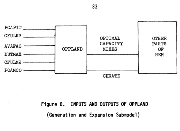
The corresponding subroutine of G&E of the FORTRAN version of REM is OPPLAND. The optimal capacity mixes of the eight plant types are

computed within the subroutine. OPPLAND takes variables listed in Table 1 of Section 2 as input variables and produces outputs as optimal

capacity mixes. As indicated in Figure 8, these variables of each plant type are exogenous except CHRATE, which is determined by other parts of

REM, is endogenous. The new installed capacity of each plant type is computed by using logic similar to that described in Section 2. The

values of optimal capacity and existing capacity of each plant type are used for such computation.

*The nine census regions are: (1) New England, (2) Middle Atlantic, (3) East North Central, (4) West North Central, (5) South Atlantic, (6) East South Central, (7) West South Central, (8) Mountain, and (9) Pacific. **The eight plants are: (1) coal-fired power plant, (2) natural

gas-fired power plant, (3) oil-fired power plant, (4) light water uranium rector, (5) light water plutonium reactor, (6) high-temperature gas

reactor, (7) liquid metal fast breeder, and (8) gas turbines and internal combustion as peaking units.

PCAPIT CFULK2 AVAFAC- OPPLAND DUTMAX CFULM2 POAMCO --OPTIMAL CAPACITY MIXES CHRATE

Figure 8. INPUTS AND OUTPUTS OF OPPLAND (Generation and Expansion Submodel)

If one is interested in investigating the effect of parameter changes on the percentage installed nuclear capacity, one would define the criterion as to what change is necessary to eliminate new

construction of nuclear capacity. In other words, one would like to do criteria sensitivity analysis similar to Case B1 in Section 2 for all nine regions and every year from 1975 to 1997. In order to do criteria sensitivity analysis, let us follow the procedure described in Section 3.

Step 1: Consider

(a) the criteria as the effect of parameter change on eliminating building any new nuclear capacity and its corresponding

indicator of performance function I(n) as the additional

OTHER PARTS OF REM

installed nuclear capacity 10 years* later.

(b) the acceptable behavior as that new nuclear capacity would not be eliminated completely from 1985 on (i.e., I(n) > 0 for any n > 1985), and

(c) all weighted coefficients for parameters as ones. Step 2:

In order to choose a direction of change of parameter vector let us compute the signs of partial derivatives of additional nuclear capacity with respect to each exogenous parameter (i.e., the signs of

aI(n)

aaj

for n = 1975, ..., 1997, where aj is an exogenous parameter).

The direction of change of parameter vector is chosen as the opposite sign of that of the partial derivatives such that I(n) would approach zero more rapidly. The direction of change** is listed in Table 15.

Table 15

CHANGE IN PARAMETERS FOR ELIMINATING NEW INSTALLED NUCLEAR CAPACITY

ALL FOSSILS ALL NUCLEAR

PCAPIT - + CFULK2 - + AVAFAC + DUTMAX + CFULM2 - + POAMCO +

*The lead time for construction a nuclear plant is 10 years.

**The direction of change is chosen for decreasing the average cost of all fossils and increasing the cost of all nuclear.

Step 3:

Since the performance function I(n) cannot be expressed explicitly in terms of exogenous parameters, one has to follow steps 4 to 6.

Step 4: Calculate the size of probable GANi.

As it is shown in Section 2, eliminating building any new nuclear plant would be more sensitive than just eliminating nuclear among optimal mixes. If one computes the least known percentage change in parameters needed for eliminating nuclear among optimal mixes, the same least known would certainly apply to eliminate additional nuclear capacity.

In order to obtain a rough idea of what the least known percentage change is, let us examine the endogenous variable, CHRATE. It is

explained in Appendix B that the increase in CHRATE would decrease optimal nuclear capacity, and conversely the decrease in CHRATE would certainly delay the elimination of nuclear among optimal mixes. Thus one can use the lower bound of CHRATE to determine the least known percentage change in parameters needed for eliminating nuclear.

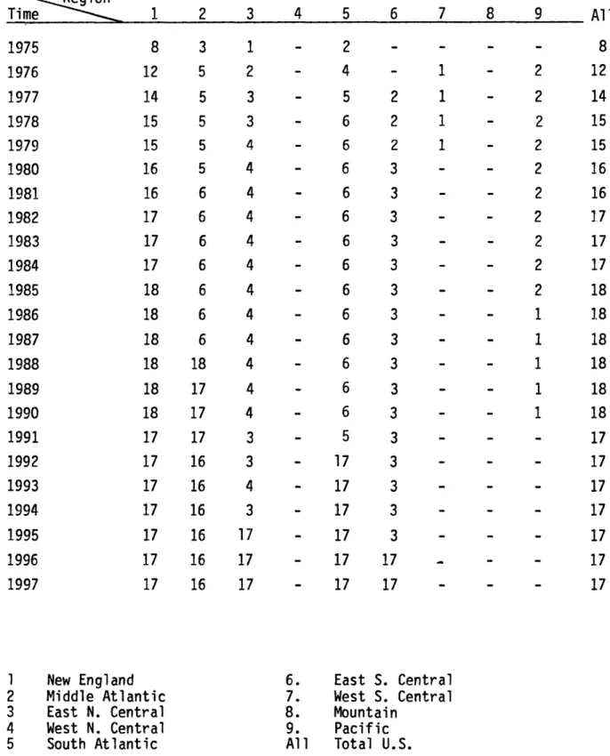
By using the computer program CALPC* and the lower bound of CHRATE (i.e., .11**) the least known percentage change needed for driving Ii(n) to negative is calculated and summarized in Table 16. Row 1 in Table 16 shows that in 1975 the least known percentage change is 12, 5, 2, and 4 for regions 1, 2, 3, and 5 respectively. For the rest of the

*The documentation of CALPC is listed in Appendix C.

**The calculation of the lower bound is shown in Appendix B.

Table 16

THE LEAST KNOWN PERCENTAGE CHANGE IN PARAMETERS NEEDED FOR ELIMINATING NUCLEAR AMONG OPTIMAL MIXES

\-, Region

Time 1975 1976 1977 1978 1979 1980 1981 1982 1983 1984 1985 1986 1987 !.988 1989 1990 1991 1992 1993 1994 1995 1996 1997 1 12 15 17 19 19 20 20 20 21 21 22 22 22 22 21 21 20 20 20 20 20 20 2 3 5 2 6 4 7 4 7 5 7 5 7 5 7 5 7 5 7 5 7 5 7 5 7 5 7 5 22 5 21 5 21 5 20 4 20 4 20 4 20 20 20 19 19 19 20 4

-

5 6 4

-- 6 2 7 3 7 4 - 8 4 - 8 4 - 8 4 - 8 4 - 8 4 - 8 4 - 8 4 - 8 4 - 8 4 7 4 7 4 7 4 7 3 20 3 - 20 3 20 3 - 20 3 - 20 19 - 19 19 7

-

8 9 All - - 12 2 - 3 15 2 - 3 17 2 - 3 19 2 - 4 19 - - 4 20 - - 4 20 - - 4 20 - - 4 21 - - 3 21 - - 3 22 - - 3 22 - - 3 22 - - 3 22 - - 2 21 - - 2 21 20 - - - 20 20 20 20 - - - 20 - - - 20 1 New England 2 Middle Atlantic 3 East N. Central 4 West N. Central 5 South Atlantic 6. 7. 8. 9. All East S. Central West S. Central Mountain Pacific Total U.S.

regions, there is no change in parameter vector because nuclear is not among the optimals in the nominal case. The last column shows the least known percentage change needed for eliminating nuclear among optimals for the entire United States. The largest number, 22, indicates that if one changes the parameter vector in the direction specified as in Table 15,

22% would definitely eliminate nuclear among optimals from 1975 to 1997. Hence, the same number, 22%, of parameter change would certainly

eliminate any additional nuclear capacity from 1985 to 1997. Twenty-two percent is the size of the probable GAN.

Step 5: Compute static results.

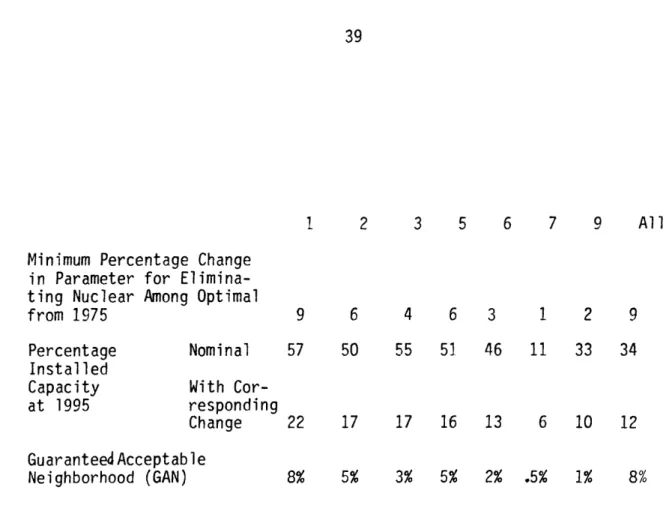
The static analysis for one region at one year in Case Al of Section 2 is obtained by using the nominal value of CHRATE. With the help of the computer program CALPC, one can easily calculate the static minimum

percentage change in parameters for eliminating nuclear among optimals for all regions and at every year from 1975 to 1997. The results are summarized in Table 17. Row 1 shows that in 1975, it takes 8%, 3%, 1%, and 2% for eliminating nuclear among optimals for regions 1, 2, 3, and 5 respectively. The last column shows the minimum percentage needed for such elimination for the entire United States. Thus the same percentage would definitely work for eliminating additional nuclear capacity 10 years from the corresponding time.

Step 6: Compute dynamic results.

The dynamic results shown in Table 18 are obtained by changing the values of exogenous parameters* within OPPLAND only for the entire period

TABLE 17 STATIC MINIMUM PERCENTAGE CHANGE IN PARAMETERS FOR ELIMINATING NUCLEAR AMONG OPTIMALS

Region

Time 1975 1976 1977 1978 1979 1980 1981 1982 1.983 1984 1985 1986 1987 1988 1989 1990 1991 1992 1993 1994 1995 1996 1997 1 2 3 8 3 1 12 5 2 14 5 3 15 5 3 15 5 4 16 5 4 16 6 4 17 6 4 17 6 4 17 6 4 18 6 4 18 6 4 18 6 4 18 18 4 18 17 4 18 17 4 17 17 3 17 16 3 17 16 4 17 16 3 17 16 17 17 16 17 17 16 17 4 5 2 4 - 5 - 6 - 6 - 6 - 6 6 6 6 - 6 - 6 - 6 6 6 - 6 -

5

-17 - 17 17 - 17 17 - 17 6 7 8 9 All - 1 - 2 12 2 1 - 2 14 2 1 - 2 15 2 1 - 2 15 3 - - 2 16 3 - - 2 16 3 - - 2 17 3 - - 2 17 3 - - 2 17 3 - - 2 18 3 - - 1 1.8 3 - - 1 18 3 - - 1 18 3 - - 1 18 3 - - 1 18 3 - - - 17 3 - - - 17 3 - - - 17 3 - - - 17 3 - - - 17 17 _ - - 17 17 - - 17 1 New England 6. 2 Middle Atlantic 7. 3 East N. Central 8. 4 West N. Central 9.

5 South Atlantic All

Note: - means nuclear is not among the

East S. Central West S. Central Mountain

Pacific Total U.S.

optimal in nominal case.

1 2 3 5 6 7 9 All

Minimum Percentage Change in Parameter for Elimina-ting Nuclear Among Optimal from 1975 Percentage Installed Capacity at 1995 9 6 4 6 3 1 2 9 Nominal 57 50 55 51 46 11 33 34 With Cor-responding Change 22 17 17 16 13 6 10 12 Guaranteed Acceptable Neighborhood (GAN) 8,

TABLE 18 DYNAMIC RESULTS PARAMETERS

1. New England 2. Middle Atlantic

3. East N. Central

9% 5% 3% 5% 2% .5% 1% 8%

WITH DIFFERENT SIMULTANEOUS CHANGES IN

6. East S. Central 7. West S. Central 9. Pacific

1975 to 1997 and then running the whole REM model without changing exogenous parameter variables in other REM subroutines. Since some of the parameters changed in OPPLAND are also used in other subroutines, the results must be interpreted accordingly, i.e. as the sensitivity of

changes in OPPLAND on REM when OPPLAND is imbedded in the overall REM structure. Ideally these results would be compared with similar sensitivity studies done when the parameter values are changed

simultaneously throughout all of REM. However, this second set of tests were not made so the differences in the two approaches are not known.

The direction of change is the same as that listed in Table 15, and the step size is .01. Row 1 shows that the dynamic minimum percentage of change in parameter vector for eliminating nuclear among optimals for the entire period of 1975 to 1997. It is the same minimum for eliminating

additional nuclear capacity from 1985 to 1997.* The New England region, which relies heavily on nuclear, requires 9% change for such elimination, while the West South Central region requires the least change, that is, 1%. Rows 2 and 3 show the percentage installed nuclear capacity in

1995. With 9% change in New England, the nuclear capacity drops from 57% to 22% and for the entire United States it drops from 34% to 12%. With

1% change in the West South Central region, the percentage installed nuclear capacity drops from 11% to 6%. The maximum size of

guarantee-acceptable neighborhood (GAN) for each region is shown in the last row. For any change of parameters within a GAN it is guaranteed

*The model is valid till 1997.

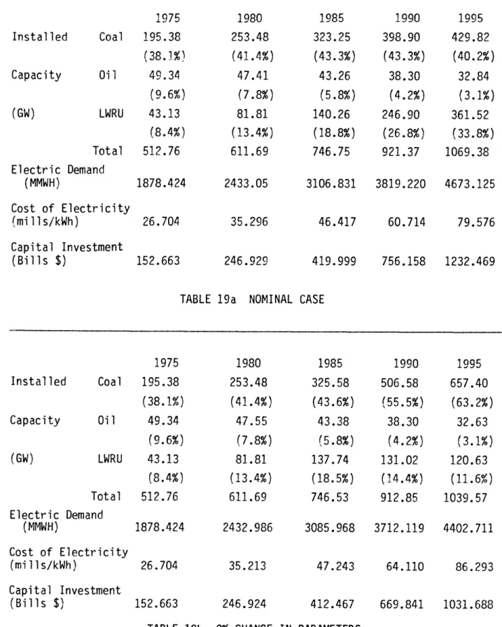
TABLE 19. DATA FOR TOTAL UNITED STATES STATISTICS IN NOMINAL CASE AND WITH 9% CHANGE IN PARAMETERS

1975 Coal 195.38 (38.1%) Oil 49.34 (9.6%) LWRU 43.13 (8.4%) Total 512.76 1980 253.48 (41.4%) 47.41 (7.8%) 81.81 (13.4%) 611.69 1985 323.25 (43.3%) 43.26 (5.8%) 140.26 (18.8%) 746.75 1990 398.90 (43.3%) 38.30 (4.2%) 246.90 (26.8%) 921.37 Electric Demand (MMWH) Cost of Electricity (mills/kWh) Capital Investment (Bills $) 1878.424 26.704 152.663 2433.05 35.296 246.929 3106.831 3819.220 4673.125 46.417 60.714 79.576 419.999 756.158 1232.469

TABLE 19a NOMINAL CASE

1975 Coal 195.38 (38.1%) Oil 49.34 (9.6%) LWRU 43.13 (8.4%) Total 512.76 Electric Demand (MMWH) Cost of Electricity (mills/kWh) Capital Investment (Bills $) 1878.424 26.704 152.663 2432.986 35.213 246.924 3085.968 3712.119 4402.711 47.243 64.110 86.293 412.467 669.841 1031.688 TABLE 19b 9% CHANGE IN PARAMETERS

Installed Capacity (GW) 1995 429.82 (40.2%) 32.84 (3.1%) 361.52 (33.8%) 1069.38 Installed Capacity (GW) 1980 253.48 (41.4%) 47.55 (7.8%) 81.81 (13.4%) 611.69 1985 325.58 (43.6%) 43.38 (5.8%) 137.74 (18.5%) 746.53 1990 506.58 (55.5%) 38.30 (4.2%) 131.02 (14.4%) 912.85 1995 657.40 (63.2%) 32.63 (3.1%) 120.63 (11.6%) 1039.57

that nuclear would not be totally eliminated druing the period of 1975 to 1997 and it is also guaranteed that some new nuclear capacity would be installed between 1985 and 1997.

Table 19 shows some of the data generated by REM for total United States statistics; Table 19a is for nominal case and Table 19b is for the case with 9% change in parameters. By comparing the corresponding data in 1995 in both cases, one notices that coal takes the place of LWRU when nuclear is eliminated completely from optimals. That is, LWRU capacity drops from 33.8% to 11.6% while coal capacity increases from 40.2% to 63.2%, yet the total capacity only decreases by 2%, that is from 1069.38 to 1039.57 GW. The electric demand drops from 4673.125 to 4402.711 mMWh, that is, a 5.8% drop. Since the cost for generating electricity from each plant type is the same as that in the nominal case, a switch from LWRU to coal would result in an 8.4% increase in the cost of

electricity, that is, the increase from 79.576 to 86.293 mills/kWh shown in the last column. Capital investment has the largest percentage

change, that is, a 16.3% drop. This is because coal plants need less capital than LWRU plants.

Table 20 shows the effect of total United States* installed nuclear capacity with different magnitudes of simultaneous change in parameters for eliminating new construction of nuclear capacity. Data from the first three rows (i.e., from 1975 to 1985) show that there is hardly any difference from that in the nominal case. It is because 10 years is the

Change in Parameters 2% 43.134 (8.4%) 81.806 (13.4%) 138.137 (18.5%) 198.963 (21.7%) 297.115 (28.1%) 4% 43.134 (8.4%) 81.806 (13.4%) 138.137 (18.5%) 171.915 (18.8%) 209.708 (19.9%) 6% 43.134 (8.4%) 81.806 (13.4%) 137.801 (18.5%) 136.876 (15.0%) 132.512 (12.7%) 8% 43.134 (8.4%) 81.806 (13.4%) 137.737 (18.5%) 131.018 (14.4%) 126.441 (12.1%) 9% 43.134 (8.4%) 81.806 (13.4%) 137.737 (18.5%) 131.018 (14.4%) 120.626 (11.6%)

TOTAL U.S. INSTALLED NUCLEAR CAPACITY WITH SIMULTANEOUS CHANGE IN PARAMETERS FOR ELIMINATING NEW CONSTRUCTION OF NUCLEAR PLANT

Nominal 43.134 (8.4%) 81.806 (13.4%) 140.256 (18.6%) 246.904 (26.8%) 361.523 (33.8%) Installed Nuclear Capacity 1975 1980 1985 1990 1995 Table 20.

Percentage installed nuclear capacity 40

30

20 10 Figure 9. hange

PERCENTAGE INSTALLED NUCLEAR CAPACITY WITH DIFFERENT SIMULTANEOUS CHANGES IN PARAMETER

lead time for nuclear construction and the model REM is designed in such a way that once the construction is in the pipeline, one cannot stop the inflow of new constructed capacity. The last two rows show that the effect becomes more significant by 1990. The percentage installed nuclear capacity is plotted against the percentage change in parameters

as in Figure 9. By comparing these two curves, one notices that the one at 1995 has a much sharper decrease than that at 1990. It implies that the effect of eliminating new construction of nuclear capacity would gradually magnify as time goes by.

Section 5: DISCUSSION AND EXTENSIONS

The implications of the results of Sections 2 and 4 relative to model validation are now discussed. It is inappropriate to try to cover all aspects of model validation (or even to try to explicitly define model validity). However, some comments on the relationship between validity and sensitivity are given. It should be emphasized that sensitivity studies can only show that a model is invalid; they cannot show that it is valid.

The concepts discussed in Section 3 can be generalized in the context of model validation by phrasing them in terms of parameter and output spaces.

Define three spaces as follows:

Parameter space: Space whose coordinates are the parameters being varied during the sensitivity studies.

Output space: Space whose coordinates are the model outputs of concern.

Differential output space: Space whose coordinates are the changes in model outputs caused by a particular policy perturbation of concern.

In each space, define a region as follows:

Parameter uncertainty region: Region (or set) in parameter space in which "true" parameter values are believed to

Output uncertainty region: Region (or set) in output space resulting from parameters varying within the parameter uncertainty region.

Differential output uncertainty region: Region (or set) in differen-tial output space resulting from parameter

varying within the parameter uncertainty region. The model maps the parameter uncertainty region into the two output

regions. Define two types of validity as follows:

Base case validity: Numerical values of outputs are valid forecasts

= predictions of what will happen under conditions hypothesized for the base case. Policy perturbation validity: Direction and magnitude of change in

outputs caused by policy perturbation are valid. Using the above definitions it can be said that a model exhibits

- Base case invalidity if the output uncertainty region is too large.

- Policy perturbation invalidity if the change in outputs caused by policy perturbation lie within the output uncertainty region (i.e., effect of noise is larger than that of signal).

- Policy perturbation invalidity if the differential output uncertainty region is too large.

The relative advantages/disadvantages of the two types of policy

perturbation invalidity will not be discussed here. It is important to note that none of these statements are the same thing as saying "a highly sensitive model is invalid." In fact, a model could also be found to be invalid if it is too insensitive to certain parameters.

The results of Sections 2 and 4 are essentially stated in terms of output space. However, it is clear that the ideas generalize readily (in a conceptual sense) from output space to differential output space.

Relative to REM itself, the numerical results of Sections 2 and 4 show that REM can be "very sensitive" to certain types of parameter changes if certain types of criteria are used. It is felt that these sensitivities have the potential for invalidating REM for certain types of studies. However, no conclusions on REM's validity are being made or

implied here. Such conclusions can only be made in the context of a particular application. Furthermore, it must be reemphasized that the numerical results were done on a version of REM that was subsequently modified.

This paper initiates a starting point to develop new approaches in parameter sensitivity for model assessment. There is no doubt that this criteria sensitivity theory can be extended to a wide-range area.

REFERENCES

1. Bode, H.W. 1945. Network Analysis and Feedback Amplifier Design. Van Nostrand: New York. Chs. 4,5.

2. Horowitz, I. December 1959. "Fundamental Theory of Automatic Linear Feedback Control Systems." IEEE Trans. on Automatic Control, Vol. AC-4, pp. 5-19.

3. Rohrer, R.A., and Sobral, M., January 1965. "Sensitivity

Considerations in Optimal System Design," IEEE Trans. Automatic Control, Vol. AC-19, PP. 43-48.

4. Cruz, J.B., Jr., and W.R. Perkins, July 1964. "A New Approach to the Sensitivity Problem in Multivariable Feedback System Design," IEEE Trans. on Automatic Control, Vol. AC-9, pp. 216-223.

5. Perkins, W.R., and J.C. Cruz, Jr. June 1964. "The Parameter

Variation Problem in State Feedback Control Systems," presented at the 1964 Joint Automatic Control Conference, Stanford

University, Stanford, California.

6. Morgan, B.S., Jr. July 1966. "Sensitivity Analysis and Synthesis of Multivariable Systems," IEEE Trans. Automatic Control, Vol. AC-ll, pp. 506-512.

7. Baughman, M.L. and P.L. Joskow. Spring 1976. "The Future of the U.S. Nuclear Energy Industry," Bell Journal of Economics, pp. 3-32.

8. Turvey, R. 1968. Optimal Pricing and Investment in Electricity Supply. MIT Press: Cambridge, Massachusetts, Ch. 2.

9. Kamat, D.P. December 1976. "Documentation of the Regionalized Electricity Model," Report from tne Center for Energy Studies, University of Texas at Austin, Austin, Texas. #78712.

APPENDIX A

1. Calculate the total cost for generating electricity from new plants only (i.e., every plant is built from scratch).

Given:

(1) average cost equation Pa.

~l+ji

u

12, ..., n

where AC - average cost (mill/kWh)

Pa - usage factor dependent component of production cost (mill/kWh)

Pb - usage factor independent component of production cost (mill/kWh)

u - usage factor (dimensionless);

(2) percentage capacity distribution among n types of plants as

P1l P2, P3, ', Pn and their corresponding maximum

usage factor and area under duration curves as u, u2, ...,

un and al, a2, ..., an correspondingly.

Then n Total Cost = Ci t=1 where

Pa

i

mill

Ci ( u 1 + Pb

u

i1 ) * a 1~~~~~~~~(mill unit mill - * unit kWh)

Example Al: Nominal Case in Section 2. Given: (1) COAL Pa Pb (2) 8.68 11.57 Capacity 23% 4% 73%

Then cost for generating electricity from Coal: (868 + 11.57) * 2.5 = 86.03 Oil: (6.979 + 17.62) * 3 = 127.64 LWRU: (11.65 + 3.771) * 128.5 = 1996.18

Total Cost = 2179.85 mill unit OIL 6.979 LWRU 11.65 17.62 3.771 1 Usage

2. Calculate the total cost for generating electricity from both existing and new plants.

Given:

(1) average cost equation Pa.'

AC.-'=

+ Pb.'

u 1 Pa." ACi" = u + Pbi" U1

for existing plants

for new plants

i = 1, 2,. .., n

(2) optimal percentage distribution among n plant types as

P1 P₂, **Pn

(3) percentage distribution among existing plants as P1',

P2', ... , e,

the total cost can be calculated as follows

(a) sum up the optimal and existing capacity into two group fossil and nuclear

(b) subtract existing capacity from optimal capacity, i.e.,

n

s

:

n

E Pi - E Pi'

i=1 i=1

(c) what is left in each group would be distributed proportionally to the positive differences (pi - pi') among plant types in each group

(d) sum up percentage capacity for each plant type as q, q2,

'.. _{qn; find their corresponding maximum usage factor wl,}

w2 , ... , wn, and compute their corresponding area under

duration curve as al, a2, ..., an for each plant type

(e) n

total cost = E C_i' + Ci" i=1 where Pa.'

c

i

'

= (

i

+

Pb

i

')

P.' * a *

i

qi

for existing plants

Pa."

ci" = ( w- + pbh") * a_i *

i

- P

)

for new plants

qi

percentage increase in total cost equals

Total Cost - Total Cost in Nominal Case

Total Cost in Nominal Case 100%

Example A2: Calculate the total cost for Case B1 (Section 2) with 7% change in parameters Given: (1) COAL Pa' Pb' Pa" 8.68 10.76 7.05 OIL 6.978 17.62 6.979 LWRU 11.725 4.035 14.413 Pb" 10.76

17.62

4.035

(2) (3) Then the total

(a)

Optimal capacity 90% Existing capacity 4%

cost can be calculated as follows FOSSIL Optimal capacity 100% Existing capacity 24% (b) 3

E

Pi-i=1 (c) Optimal capacity Existing capacity Difference 3

E Pi'

i=1 COAL 90% 4% 86% = 100% - 64% = 36% OIL 10% 20% -10% LWRU 0% 40% -40% (d) Existing capacity New capacity Total capacity Usage factor Area COAL 4% 36% 40% 1 51.5 OIL 20% 0% 20% .15 1.5 LWRU 40% 0% 40% 1 80

(e) cost C_i' from existing plants

COAL: (8.68 + 10.76) * 5.15 * (4/40) = 100.12 OIL: ( -1- + 17.62) * 1.5 * (20/20) = 96.22 10% 20% 0% 40% NUCLEAR 0% 40% qi

W.

a_i

LWRU: (11.725 + 4.035) * 80 * (40/40) = 1260.77 cost Ci." from new plants

COAL: (7.05 + 10.76) * 51.5 * (36/40) = 825.49

Total Cost = 2282.60 mill unit

percentage increase in total cost equals 2282.60 - 2179.85* * 100% = 4.7%

2179.85

*2179.85 is the total cost at nominal value calculated in example B1. The percentage increases in total cost with different simultaneous changes in parameters are indicated in the second last row of Table 14, Section 2.

APPENDIX B

1. Let a be the multiplicative change in CHRATE, i.e. new CHRATE = a * nominal value of CHRATE.

For the nominal case, the average cost equation is given as:

Pa. C. = + Pb. 1 U 1 and Pa. - Pak L(USEVAL)= -P:-a a Pak - bj for i = 1, 2, ..., n for j k.

If a 1, then the new average cost equation is: Pa. * a

Ci= -

_{i- U}

+ Pb

_i~

and the corresponding Pa. - Pak USEVAL = - * a

Pbk - Pbj

a > 1 -- > SEVAL shifts to the right as indicated in Figure B; and a < 1 = USEVAL shifts to the left.

Cost

~V

C¢i

(L , It. p Usage

Figure B.

I

If the USEVAL is the intercepting point between fossil and nuclear, and both plants are among optimal mixes, it implies that the increase in CHRATE would decrease the optimal nuclear capacity, and conversely the decrease in CHRATE would increase the optimal nuclear capacity.

2. Calculate the lower bound of CHRATE

Capital charge rate CHRATE in REM is defined as:

D *

DINTN + (TE

* Re

+ PS

* PINTN)

CHRATE +1 - TAXINC

CHRATE

:~+

... D

+

TE

+

PS

where D DINTN TE Re PS PINTN TAXINC L Lower bound of total = .085, = total = .14, = total = .085, = .30, = 40, CHRATE debt capital

interest rate on new debt capital equity capital

regulated return on equity preferred stock capital

interest rate on new preferred stock taxing rate lifetime of plant D * .085 + (TE x .14 + PS * .085) 1 1 - .30

I-U

- +

D

+ TE

+ PS

= 1/40 + .085

- .11

lim TE + 0 PS + O

APPENDIX C

DOCUMENTATION OF PROGRAM CALPC C PROGRAM CALPC

C THIS PROGRAM IS USED FOR STATIC ANALYSIS: C TO CALCULATE C (1) C C C C C (2) C

THE APPROXIMATED LEAST KNOWN PERCENTAGE CHANGE IN PARAMETER VECTOR NEEDED FOR

ELIMINATING NUCLEAR AMONG OPTIMAL MIXES,

(i.e., THE SIZE FOR PROBABLE GUARANTEED ACCEPTABLE NEIGHBORHOOD GAN)

THE MINIMUM PERCENTAGE CHANGE IN PARAMETER VECTOR FOR ELIMINA-TING NUCLEAR AMONG OPTIMAL MIXES.

C

DIMENSION PA(9), PB(9), USEVAL(12), IPLANT(10) DIMENSION DM(9, 54), PCM(54), t-WD:Q, XX(50).

C

C INITIALIZATION

C

C NSC = 1 IS USED FOR CALCULATING THE SIZE OF PROBABLE GAN NSC RTN RTE IDP = O = 1975 = 1998 = 50 C LOOP THROUGH TIME

DO 580 NCT = 1, 54 C READ DATA

100 IF (RTIME.GT.RTE) GO TO 900

IF (RTIME.EQ.RTE. AND IREG. EQ. 9) GO TO 600

READ (8, 10) (PA(I), I = 1, 8), CHRTE, NUS, NUSMO, KYEAR, *1REG, RTIME

READ (8, 11) (PB(I), I = 1, 8), (USEVAL(I), I =1, NUS) READ (8, 12) (IPLANT (I), I = NUSMO)

IF (KYEAR.EQ.2.0R.RTIME.LT.RTN) GO TO 100

C USE LOWER BOUND .11 OF CHRTE FOR FINDING THE SIZE OF PROBABLE

C GAN IF (NSC.NE.1) GO TO 300 DO 190 J = 1, 8 190 PA(J) = (PA(J)/CHRTE) * .11 C C MAIN PROGRAM C

C OBTAIN NUCLEAR PLANT TYPE IN OPTIMAL MIXES 300 INU = O INUP = 0 IPID = 0 DO 310 I = 1, NUSMO IF (IPLANT(I).LT.4.0R.IPLANT(I).GT.7) GO TO 310 IPID = I INU = IPLANT(IPID) INUP = IPLANT(IPID - 1) GO TO 400

310 CONTINUE

C CALCULATE THE PERCENTAGE CHANGE FOR EACH REGION AT EVERY TIME

C

C IF NUCLEAR IS NOT AMONG THE OPTIMAL MIXES, SKIP THE CALCULATION 400 IF (IPID.EQ.O) GO TO 580

C OTHERWISE INCREASE THE COSTS FOR NUCLEAR PLANT AND DECREASE COSTS C FOR FOSSIL WITH STEP SIZE 1 PERCENT

DO 430 I = 1, IDP D = .01 * (I -1) PAIN = PA(INUP) * (1. - D)/(1. + D)**2) PAJN = PA(INU) * (1. + D)/(1. - D)**2) PBIN = PA(INUP) * (1. - D) PBJN = PB(INU) * (1. + D) C CALCULATE USEVAL

XINT = (PAIN - PAJN)/(PBJN - PBIN) XX(I) = XINT

C IF USEVAL > 1, STOP LOOPING IF (XINT.GE.1) GO TO 500 430 CONTINUE

C RECORD THE PERCENTAGE CHANGE FOR EACH REGION AT EVERY TIME 500 DM(1REG,NCT) = D

C RECORD THE PERCENTAGE CHANGE FOR U.S. TOTAL DO 510 I = 1, 9

510 IF (PCM(NCT).LT.DM(I, NCT)) PCM(NCT) = DM(I, NCT) C IF (RTIME.EQ.RTE.AND.IREG.EQ.9) GO TO 600

580 CONTINUE

C WRITE THE MATRIX OF PERCENTAGE CHANGE FOR EVERY REGION AT EVERY TIME 600 DO 610 I = 1, NCT

RTIME = RTN + (I - 1) * .5)

WRITE (3, 22) RTIME, (DM(J, I), J = 1, 9) PCM(I) 610 CONTINUE C FORMAT STATEMENT 10 FORMAT (8(G11.4, 1X), 3X, F8.5, 313, I7, F8.1) 11 FORMAT (8(G11.4, 1X), 3X, 4F8.5) 12 FORMAT (99X, 418) 22 FORMAT (F.10.1, 10F6.2) C 900 STOP END

APPENDIX D Changes made in subroutine OPPLAND:

After line NBJ00390 ( i.e., IF(KYEAR.EQ.2.AND.K.EQ.4) J = 8) insert statements as follows

--IF (KYEAR.NE.3.0R.J.GE.8.OR.RTIME.LT.1975.0) GO TO 50 C PC IS PERCENTAGE CHANGE

PC = .01

IS = 0

C DECREASE COST FOR FOSSIL AND INCREASE COST FOR NUCLEAR

IF (J.LE.3) IS = -1

IF (J.GE.4.0R.J.LE.7) IS = 1

D = PC * IS

PA(J) = CHRATE(IREG) * ((PCAPIT(J, KYEAR)) * (1. + d)

*

+

CFLUK2(J) * (1. + d))/(8.76 * AVAFAC(J) * (1 - d) * DUTMAX(J)

* '*(1. - D))

PB(J) = (CFULM2(J, KYEAR)+ POAMCO (J, KYEAR)) * (1 + d) GO TO 1

O (- C C) C) r-t F-he..w F' CL1

0

r

ri

_j

-rt (t ri r C -C:) C)C) ct ct - C) F n rt f-t H' I-" 9 ol' C, , j t> J L4 \- IN-) "-J T o

O

'- F'i) Ui0

lC

l

W

CoI \L) O Ul l N) CO --.1 C

00

HI H' Ct r l-HD (4 G1 N ' -4 l- j I t-' --r-. n W 0 W - . H (S D t W W t-' O 00 r,

00

- O

F

-

₀

_Cl

_-

_CN

W " . - 00 o H. - - C- Ln H l n 0D W

an

o O -a -W t-' 4 H t- N) O CO 0 c P W 0n O F-o ..-O- . 0 4-- 04ŽCo -'4 1 C H - --'D -I \D _-N) to _(4n ln co P- 11. _{I'D~1 i} O (,)₀ 'O- 0 coN) -j 1 H t(n tn 10 Do Co - 'o O Ln ro n --J CO .) . 1 0 L I' _> ,P 0 o O -H O4) iN H O HO H C

O

H

O--- 4>I O F' C) -O F-0 O ( 0C (--4 c o) HO '-D N) '--J C-, .) ) o r 'W i- (-CO C, 0~, (£. , u. kn (4 1 0 . '- u 0) 0 D

'.

-,)

C)

0',

.)

a

Ž.-. O o H G -4 '- 1) 0 0 -C" CO 4D Ln -.J ka 4-t) LO (41 (4) J 4>

I

-. r t, C) C) H w -C (C C) LTi i4 (2 H kO_-' UD Hi '-2Q rt tt Cc) 10 "i P 0 c) C) rr rt 'A4 H 'I H (2 C-C) (> Ft-t3_FD H H I-ti H~ H Ln W H ,-Co O Fd tH F-0n_C) (TI C' 0F-H _O O r - 4---4 L-' t.' (4 t.)

1 C O r 0 t rt - . rt PJ J P ~ ' H- - H- H' rt t rt rt

r

0 trt -H c. n n

I0 0

PI) _F0 Cp) H- e-rt rr r· ;:-O o t-7 J C) H- H-rt H-rt 1-1: 4 .- W P t' N H -- H ONO -ln O IN W b I > ULn 1n 1 0o J O P), -C r rt- t

ri

IO .--Ln H 1-1 oll ' -D> CO W - ,H -H . '

H1

D

0

O

UO

Fc

cU

Oh0

· t.,

W>

H

O

- -

- U

W r 0 O 4>- P U i H

0

-n O 00 _o Ul _0',-J 'n. OlI I ,) 0" a'. -i0 \J] Ul to Cn

UH

"r_

*

oU

N\ ON O N) O io -4 Co

H r

*0 W O~a CI-n 1 Ul Ul O H N)O. O >--04 >O O \D 0co H tn-J Wn '> W O'n * ON a .. O ON

o co

_.

_{w 00 .}

\0

)

_'

_o

o

0o -CO O CX 00 .n P O b - \O tr 4'-I I I I I I I I H co LI > C I. u] H O O H O) .

--i

coc HO -OH . J-1 t-- OC F- ,0 -- H ca-) JI C) G\ C) . i -' (.J O' -j W C0) C') Jl W C- C CT,

Li

' C

-)

a \ 2 -) Cn l W ·J t_ e- tl H Cl_rH r] PO O Cd C3 H H

o

H H C) tJ U) 1 r t4 t7') t~i C) tH H F-tZ Qr m3 0N -. I

t'

L-rt rt r-t -C3 1Jt cH H Ct -T Nt r 4N b. _{co )} O' bo bbH HL NO O OC O

I !

I !

0r C) \n i--H1) (-2 4Ž1- (~ 0O'H~ .-7) I) [) 0 -i A n 4 ) ) Co n o o-cD 00_'o 00 Cn t-CO to r N ) n G tt Ln

0 0

I I I I - -J

I-IUJ

VN -u) V CO

0

rt _ri -0D f L rt rt Fo ) O HO ) 0 4

O

0 O'xO 0 'JD H- H.

_{O r}

C 00 F-t-, P-0 P-0P-0_ri4--.) k * 4 . O O I-00 I I I I II I I Ho coCD UL -ci 4. U- .4=-t-4l t-_nn 0 w C)1< H H H, r C) t H tt, Cr L. w H C-I C)m_u O O t-4 m PU Cxl

e

H O H t-t =tJ C)

0

H ~o O CII

₀

H

0

z

C)

n

F-4

0

Zx w Io( C) :31 OQ CL Ln -3 Co a' --'. C-I

-H t-\0 X,

o r

.O

-Ct :. rt -nO C 'n H rt rt OLn

n

-0

r

rt ? H *k CO O t-4 rt -fC C) n n rt s :CC CO

r

0

O O 1' r-t n n C iO I, 3 W) F N H t' U 0) N H N. '-4 k0 G\ _{P-O U,} . lx ₎ '0 ₀₎ '_LI) O'> 4 o w -H

CFo

>O H 4>-O 0 - C O n O 4Ž- O 4 >0 4--lj w Go -1 * CT F-' N)iN) K -) ULi LI '-N 1 Co *~ n CO W co aHH0'ZJO F~-H _C00 -04 *

-ro

F O n 'D F-4 .₀ t-I_r r-

:-C

noZ C) C n H rt rT -D -H. -" I- GEN

OUn O- N) I'D 'IT,O O

4S -n <D O o H kn C) 0-> - --'.O F -4 ' D O I. k, O cO W

II

II

II

II

I I

I I I I II I I I I

II

I I

I I

It

'.0 H -4 H Ot -1 G~ C-Co . H .

-.

L , W ul 4 1-0 F- C0, c? Co O) CD kn HI4--n w -1< C·' H O. H i-3 , t-rC _7 t., H 4 R3 w tI > t-H F-3

z

H C D tJ t-3 m H

o

Hd

0

p

H

z

trl rr U)j

o

i._ix) ! OC o. .o Co_D t-* ' I:- U-4 I

H fo _{0 )} F- H-fn r H' H' rt rt L~ -J Co Ft :;, 10 rt z-l H : H C)C) C)C) rCt rt Ct 4-'- "

4L-- -I C.

(1) H

* * *

3 f

.

-j

W H C C G Co . ' 00 Co H O Ln W 0\ £D 'O CO 0\ k r t, Hn

UiH

H O' '0O LO- -J 0 O " -O' H 1- LIH 0 I£ - t t'.3 - H H O U- C"O O Co020 H 0'- 0 - -- Ln

II

I I

II

tn W co co O WU -IC co io (.,o id I I I I 'D - -4 . Z N.O w - D t" k I I I I I I I I I I II I I I I I I I I I I I II I I I I -- ' 4 'n -, -JI W cT . o cD C CL) \ 0 Un L. I ) (-.) J H L1 Uc V) H Iz t- t-trl C) H H Un '.0

,-or

n _or rt

_"

_c;

e' Hb C3 rt rt ,.<4 ,-.< H c 0 rt , . tD; n 0 rl r H t'd tri Ln H p> t-4

tl

C) tr

n

H3 O H

t--r

H tTJ H o' W O H W 07 --4 U. H C o- 0 UI _O'C'0'0

1wt

O --J ' 1O--'