HAL Id: hal-00999849
https://hal.archives-ouvertes.fr/hal-00999849
Submitted on 6 Jun 2020HAL is a multi-disciplinary open access archive for the deposit and dissemination of sci-entific research documents, whether they are pub-lished or not. The documents may come from teaching and research institutions in France or abroad, or from public or private research centers.
L’archive ouverte pluridisciplinaire HAL, est destinée au dépôt et à la diffusion de documents scientifiques de niveau recherche, publiés ou non, émanant des établissements d’enseignement et de recherche français ou étrangers, des laboratoires publics ou privés.
Estimating the causal effects of the French
agro-environmental schemes on farmers’ practices by
difference in difference matching
Sylvain Chabe-Ferret, Julie Subervie
To cite this version:
Sylvain Chabe-Ferret, Julie Subervie. Estimating the causal effects of the French agro-environmental schemes on farmers’ practices by difference in difference matching. OECD Workshop on Evalua-tion of Agri-Environmental Policies, OrganisaEvalua-tion de CoopéraEvalua-tion et de Développement Economiques (OCDE). FRA., Jun 2011, Braunschweig, Germany. 19 p. �hal-00999849�
1
OECD Workshop
on the
Evaluation of Agri-environmental Policies
20-22 June 2011The Johann Heinrich von Thünen Institute, Bundesallee 50, 38116 Braunschweig, Germany
Monday, 20 June Session 3a : 14h30-18h00
Estimating the Causal Effects of French
Agro-environmental Schemes on Farmers’ Practices
Sylvain Chabé-Ferret and Julie Subervie
Estimating the causal effects of the French
Agro-Environmental Schemes on Farmers’ practices
by Difference in Difference Matching
∗
Sylvain Chabé-Ferret
†‡and Julie Subervie
§May 2011
Prepared for the OECD workshop on the Evaluation of Agro-Environmental Policies 20-22 June 2011, Braunschweig, Germany.
Abstract
We present the first disaggregated estimation of the causal effects of a nationwide AES program on environmentally-relevant practices for a nationally representative sample. We study the AES program that has been implemented in France between 2000 and 2006 as part of the EU policy for rural development. The causal effect of the AES program is the average difference between practices of participants in the presence of the program and what their practices would have been had the pro-gram not been implemented. This counterfactual situation cannot be observed and intuitive approximations using non participants’ practices or participants’ practices before receiving the AES are plagued by large sources of bias (selection bias and time trend bias). To correct for these sources of bias, we use Difference-in-Difference (DID) matching. The main idea is to compare each participant to a non participant "twin" with the same observed characteristics. We combine matching with DID to correct for any remaining bias that may be due to unobserved variables. Our results suggest that the size of windfall effects of the AES programs depends on the specific prerequisites for each AES. For example, the AES supporting conversion to organic farming, which combined large payments with the strong requirement of not being an organic farmer when applying for the AES, have had negligible windfall effects. We cannot conclude on the extent of windfall effects of payments for exten-sive herding. We provide a first attempt to integrate the results of causal analysis in a cost-benefit evaluation of the AES. We argue that evaluation should be prepared at the same time the program is designed. This would improve the collection of data and enable using the first results of the evaluation to design the next program (by suppressing or altering the less efficient AES). Finally, this could allow for the implementation of experimental methods to evaluate policies that do not comply with the assumptions of DID-matching, like payments for extensive herding.
∗We gratefully acknowledge financial support from the French Ministries of Agriculture and
Sustain-able Development.
†Cemagref, Umr Métafort, Aubière, France.
‡Corresponding author. Correspondence to: Cemagref, Umr Métafort, Campus
Univer-sitaire des Cézeaux, 24 avenue des Landais, BP 50085, 63172 Aubière Cedex, France. Email:
sylvain.chabe-ferret@cemagref.fr.
1
Introduction
Payments for environmental services are widely used to improve environmental outcomes. Agro-environmental schemes (AES), consisting in paying farmers who volunteer for adopt-ing practices more favorable to the environment, are increasadopt-ingly important components of environmental and agricultural policies both in the US and the EU. We present the first disaggregated estimation of the causal effects of a nationwide AES program on environmentally-relevant practices for a nationally representative sample. We study the AES program that has been implemented in France between 2000 and 2006 as part of the EU policy for rural development.
A complete cost-benefit evaluation of AES requires estimates of the causal (or addi-tional) effect of the AES and of the extent of windfall effects. We define the causal effect of the AES program as the average difference between practices of participants in the presence of the program and what their practices would have been had the program not been implemented (i.e. the counterfactual situation). The counterfactual level of prac-tices is also a direct measure of the windfall effect. Farmers indeed receive payments for the overall level of their practices, thereby receiving payments also for adopting practices that would have adopted even in the absence of the payments.
When trying to estimate the causal effect, we face a major problem since the counter-factual situation cannot be observed and thus has to be approximated thanks to observed data. Usual approximations are plagued by what may be large sources of bias. To correct for these sources of bias, we use Difference-in-Difference (DID) matching to estimate the causal effects of the French AES. The main idea is to compare each participant to a non participant "twin" (i.e. a non participant with the same observed characteristics): if a sufficient number of characteristics can be used, the average difference between partici-pants’ and non participartici-pants’ practices estimates the causal effect of the program. This identification strategy relies on three main assumptions. First, non participants’ practices have not been altered by the program. Second, for each participant a non-participant twin exists, which means that observed characteristics used for the matching are not the only variables explaining the participation to the program and that other unobserved characteristics exist (like managerial ability or environmental awareness). We combine matching with DID to correct for any remaining bias that may be due to these unob-served variables. This approach amounts to subtracting from the difference obunob-served after the program was in place between participants and their "twins" the difference between the same farmers that existed before the program was in place. Third, the difference in practices due to unobserved variables has to be constant through time.
Our results suggest that the size of windfall effects of the AES programs depends on the specific prerequisites for each AES. For example, the AES supporting conversion to organic farming, which combined large payments with the strong requirement of not being an organic farmer when applying for the AES, have had negligible windfall effects. We cannot conclude on the extent of windfall effects of payments for extensive herding, because we find evidence of violations of the identifying assumptions for these AES. We use these estimates of additional and windfall effects to attempt a first cost-benefit analysis of some of the French AES.
We make some suggestions aiming at improving the evaluation of future programs. We argue that evaluation should be prepared at the same time the program is designed. This would improve the collection of data and enable using the first results of the evaluation to design the next program (by suppressing or altering the less efficient AES). Finally, this
could allow for the implementation of experimental methods to evaluate policies that do not comply with the assumptions of DID-matching, like payments for extensive herding. This paper is organized as follows: section 2 quickly presents the AES implemented in France between 2000 and 2006; section 3 defines causal effects, the problem we face when estimating them and how DID-matching solves it; section 4 presents the data used in the analysis; section 5 presents the estimates of the causal effects of the AES on agricultural practices and makes an attempt at inserting the causal estimates in a cost benefit framework; section 6 discusses some extensions and section 7 concludes.
2
Agro-Environmental Schemes in France
Agro-environmental schemes (AES), consisting in paying farmers who volunteer for adopt-ing practices more favorable to the environment, are increasadopt-ingly important components of environmental and agricultural policies both in the US and the EU. Rural development policies accounted for 22 % of public spending for the Common Agricultural Policy of the European Union in 2006, and AESs accounted for 37 % of rural development spending (Pufahl and Weiss, 2009). In France, these figures are lower (resp. 17 % and 25 %), because of a lower use of these schemes in public policy and historically high levels of direct support.1
French AESs are nevertheless worth assessing for two reasons: first, their share of total public expenditure on agriculture has steadily increased since 1992, when they were first introduced (for example, public spending for AESs nearly doubled between 1999 and 2006). Second, France being the main beneficiary of agricultural policies in the EU, even a small proportion of the total budget represents a large amount of money. In 2006, 521 million Euros were spent on AESs in France, accounting for roughly 1 % of total CAP expenditures for the EU as a whole (AND, 2008). Finally, if AES expenditures in France per hectare of usable agricultural area (UAA) are lower than in most European countries,2
it is mainly because the area affected by AESs is smaller than in other coun-tries, and not because payments per hectare in an AES are small. Estimating the impact of AESs in France is therefore an important step towards measuring the effectiveness of agro-environmental spending in the EU. In France, AES were implemented between 2000 and 2006 as part of the National Plan for Rural Development (Plan de Développement Rural National (PDRN)) as five-year contracts, with yearly payments and possible con-trol of how well the requirements are met. The main way for farmers to benefit from an AES during this period was to submit a written application containing an environmental diagnosis of their farm and the particular measures they were applying for. An admin-istrative authority then had to approve or refuse the application. AESs were referred to with a seven digit code: the first two digits referred to the general category of the AES, the following three referred to the particular requirements the farmer had to meet to enter the AES and, finally, the last two digits referred to the regional variation in the AES. The two-digit codes of particular relevance for our study are AES 02 (diversification of crop rotation), 03 (sowing of cover crops), 04 (planting of grass buffer strips), 08 (reduction in the use of pesticides), 09 (reduction in the use of fertilizers) and 21 (conversion to organic farming). Taken together, these AESs accounted for 22 % of total spending on AES in 2006 in France.3
These AES are presented in table 1.
1
According to the French Ministry of Agriculture’s website.
2
According to the European Environment Agency’s website.
3
Subsidies for extensive farming of meadows accounted for 60 % of total spending for the AES in France in 2006. As described in Chabé-Ferret and Subervie (2009), the methods applied in this paper
3
The fundamental problem of causal inference and
how DID matching solves it
3.1
The definition of causal effects
We define the causal effect of the AES program as the average difference between practices of participants in the presence of the program and what their practices would have been had the program not been implemented. This latter unobserved situation is called the counterfactual situation. This notion captures the intuition that underlies most of the analysis of causality: a causal effect is the consequence of a ceteris paribus change, here the implementation of an AES program. Figure 1 illustrates this definition: the causal effect of the AES is the difference between the practices observed in the presence of the AES (materialized by a continuous line) and the practices that would have been observed had the program not been implemented (discontinuous line). In this paper, we are interested in the effect of the AES on those who chose to enter it. As most of this literature stems from biostatistics, we refer to the policy evaluated (the AES) as a treatment, and thus the causal effect we are after is termed average treatment effect on the treated (ATT).
Figure 1: Treatment effects and selection bias
Time A gr ic ul tu ra l pr ac ti ce s t-2 t-1 t Treated Time of treatment Counter-factual
Causal effect (ATT)
Untreated
Selection bias Before receiving AES
Time trend bias
3.2
The fundamental problem of causal inference
When trying to estimate this causal effect, we face a major problem since the counterfac-tual situation cannot be observed and thus has to be approximated thanks to observed data. Usual approximations are plagued by what may be large sources of bias. The comparison of the participants’ practices to those of non participants suffers from “se-lection bias”: it is likely that participants who self select into the program would have adopted practices greener that the ones of the non participants had the program not been implemented. Figure 1 illustrates this bias: in the absence of the AES, those who end up receiving it would have had higher practices than the untreated. This is because
cannot be used to estimate the impact of these subsidies because most of the eligible population benefits from them, so that they tend to affect non-participants as well, mainly through the land market.
complying with the requirements of the AES is less costly for those who would adopt favorable practices in the absence of the AES.
Selection bias is due to the fact that treated and untreated farmers differ in char-acteristics that determine their agricultural practices. These charchar-acteristics may either be observed by us (like education, type of farm, capital, land. . . ) or unobserved to us (as environmental preferences or managerial ability). Selection bias may accordingly be divided into two types: selection on observables and on unobservables.
The comparison of the participants’ practices before and after the beginning of the program suffers from a “time trend bias”: the practices would have changed even in the absence of the program since other determinants of farmers’ practices as input and output prices have indeed changed between this two dates. This is illustrated in figure 1: observed practices for the treated have decreased, which would be interpreted as a negative causal effect of the AES. But the practices would have decreased by much more in the absence of the AES, so that the causal effect of the AES is in fact positive.
3.3
Identification of treatment effects by Difference in Difference
matching
We use DID matching to get rid of biases. The first type of selection bias, due to observable variables, is eliminated by comparing treated farmers to “twin” untreated farmers that have the same values of the observed characteristics. This is the method of matching (Imbens, 2004), that we present in more details in (Chabé-Ferret and Subervie, 2010). Unobserved variables may still bias simple matching estimators, as illustrated in figure 2: the agricultural practices of the untreated “twins” are closer to the counterfactual ones, but some difference remains that would lead to overstate the causal effect of the AES. For example, treated farmers may be more environmentally conscious and thus have better practices in the absence of the AES. But environmental awareness is not measured in our databases and thus cannot be controlled for by matching. We estimate selection on unobservables by comparing the practices of the treated before entering the AES to the ones of their untreated twins at the same date. We then subtract the difference in practices estimated by matching before the AES has been implemented from the difference estimated after. This method is thus called Difference in Difference (DID) matching (Heckman, Ichimura, and Todd, 1997). The example on figure 2 illustrates the method: the difference in practices at period t − 1 between treated and untreated twins is equal to the difference that would have been observed in period t had the AES not been implemented.
This method also gets rid of time trend bias by comparing the evolution of practices of treated farmers to that of their untreated twins. This is illustrated on figure 2: the counterfactual decrease that would have occurred to the treated had the AES not been implemented is mirrored in the decrease that occurred to the untreated twins. In fact, we can indifferently implement DID-matching by comparing the change in practices that the treated experienced to the one experimented by the untreated twins, or alternatively compare how difference between treated and untreated twins changed after the AES has been implemented.
This identification strategy relies on three main assumptions. First, non participants’ practices must not have been altered by the existence of the AES program. This rules out imitation effects or diffusion effects but also effects of the AES on input or output prices. This assumption seems coherent because imitators would also be likely to apply
Figure 2: Identification of treatment effect by DID matching Time A gr ic ul tu ra l pr ac ti ce s t-2 t-1 t Treated Time of treatment Counter-factual Causal effect Untreated Untreated twin
for an AES to get compensated. Secondly, for each participant a non-participant twin exists, which means that observed characteristics used for the matching are not the only variables explaining the participation to the program and that other unobserved charac-teristics exist (like managerial ability or environmental awareness). Thirdly, we assume that selection bias on unobservables is fixed through time. This is a rather important assumption, but we test it in the longer version of this paper (Chabé-Ferret and Subervie, 2010) and find support for it. The test uses another pre-treatment observation (as period t− 2) in figure 2 and compare selection bias in both periods.
4
Data
The empirical analysis is based on a longitudinal data set constructed from a statistical survey on agricultural practices conducted in 2003 and 2005 by the statistical services of the French ministry of Agriculture (named “STRU” 4
) paired to both the 2000 Census of Agriculture (“CA-2000”) and several administrative files recording information on the participation in the AES between 2000 and 2006. The data in “STRU-2005” are used to measure post-treatment outcomes, those in “CA-2000” are used to build both pre-treatment outcomes and control variables, and the data in “STRU-2003” serves for the robustness tests. This is an original database built especially for this work. Its construc-tion involved a pairing procedure based on several steps because of the scattering of data. The sample extracted from “STRU” is representative of French farmers.
4.1
Definition of the participation variables
For each AES, participation is a binary variable taking a value of one when the surveyed farmer appears in administrative files as receiving subsidies compensating him for coping with the requirements of the AES between 2001 and 2005, and a value of zero when the surveyed farmer does not appear in the administrative between 2000 and 2005. The few farmers receiving an AES before 2001 are excluded from the sample, because no pre-treatment observation exists for them. Because farmers may benefit from several AES,
4
the participation variables partially overlap. This is generally not a problem because the AES that are correlated with each other aim at influencing different practices. When two AES may have an impact on the same outcome variable, we study their effect separately by focusing on the sets of participants that only benefit from each one of them. Table 1 reports the sample size and the number of participants for the AES we study in this paper. The sample contains between 400 to 3,000 participants depending on the AES, which represents between 2,000 and 14,000 participant farmers nationwide. We also have access to almost 60,000 non-participants, representing 540,000 farmers nationwide.
Table 1: Samples size and AES participation
AES Restriction imposed Treated CS(a) Non treated Sample
0301 Implanting cover crops 1,811 1,617 58,951 60,568 09 Reduction of fertilizer use 3,173 2,824 58,951 61,775 08 Reduction of pesticides use 3,197 2,849 58,951 61,800 04 Implanting grass buffer strips 1,532 1,356 58,951 60,307 0201 Adding one more crop to the rotation 446 382 58,951 59,333 0205 Having at least 4 crops in the rotation 1,844 1,635 58,951 60,586 21 Conversion to organic farming 720 536 58,951 59,487
Notes : (a) CS refers to the estimated number of treated on the common support, i.e. for whom some untreated twins exist. Details of its calculation can be found in Chabé-Ferret and Subervie (2010).
4.2
Definition of the outcome variables
The average treatment effect on the treated is estimated for five AES. Several outcome variables are associated with each AES. Two outcome variables allow us to estimate the impact of the measures 03 and 04 which aim at reducing nitrogen carrying by rain drainage: the land area dedicated to cover crops for soil nitrate recovery and the length of fertilizer-free grass buffer strips located at the edge of agricultural fields which attenuate nitrate lixiviation. As cover crops may be a way to retain nitrogen during winter, we study whether farmers participating in AES 09 aimed at curbing the use of nitrogen fertilizers have an increased use of cover-crops, even when they are not participating in AES 03. The impact of the AES 02 encouraging crop diversification is measured on three outcome variables: the proportion of the total land area dedicated to the main crop, the number of crops, and a crop diversity index.5
Finally, we use two outcome variables to estimate the impact of the measures, which aim at encouraging conversion to organic agriculture: the land area dedicated to organic farming and the land area under conversion. All areas are measured in hectares.
4.3
Definition of control variables
Crucial for the relevance of both matching and DID-matching identification strategies is the set of pre-treatment observed variables we use to select non-participants observation-ally identical to participants. The richness of the information in our database enables us
5
We use a regularity index, which is an evenness measure of crop diversity, independent of the number of crops and dependent solely on the distribution of land area among the crops.
to control for most of the important determinants of input choices and selection into the program listed in our theoretical model. On the production side, we have access to a very detailed description of the equipment (tractors, harvesters, etc.), buildings, herd size and composition, land area, slope, altitude and type of land at the level of the commune6
(Jones et al. 2005, Metzger 2005, Hazeu 2006), size of the labor force, age and education level of farm associates, etc. On the consumption side, we have data on the composition of the household, the main non-farm activity of the farmer and his spouse, etc. The dataset also includes measures of technical orientation of the farm, labels of quality, past experience with the previous AES (1993-1999) and other agricultural policies.7
The main unobserved variables are thus managerial ability, ecological preferences and prices.
5
Estimation of causal effects and cost benefit analysis
of the individual AES
In this section, we present the results from the matching and DID-matching procedures and insert them into a cost benefit framework. We only present results for the simplest estimators and do not detail the procedure we use. See Chabé-Ferret and Subervie (2010) for more details on the estimation procedure.
Matching is implemented by selecting, for each treated farmer, a twin untreated farmer that has observed pre-treatment control variables as similar as possible to the treated farmer. Similarity is measured by an Euclidean distance (sum of squares of the difference in control variables, normalized by the variance of each variable). The twin untreated farmer, or nearest neighbor, is the one with the lowest distance to the treated farmer. Once the twin is selected, we form the difference in outcomes between the treated farmer and its twin. By doing this for all treated farmers and taking the average of these differences, we estimate the average causal effect of the AES on the treated farmers (ATT).
DID-matching is implemented using the same procedure, but instead of comparing outcomes in levels, as in matching, we compare differences in outcomes before and after the treatment date (2000 and 2005 in our application). This differencing gets rid of all remaining pre-treatment differences between treated farmers and their twins due to unobserved variables.
In this section, we present in turn results from simple and DID-matching and then a tentative cost-benefit analysis.
5.1
Results from simple matching: measure of the extent of
se-lection on observables
Table 2 presents the result that we obtain by comparing the practices of treated farmers to the one of twin untreated farmers having the same characteristics, i.e. by applying simple matching. In the third column of the table, we present the mean outcomes of all untreated farmers and in the fourth column the mean outcome for treated farmers. The difference between these two quantities forms the with/without comparison, that is plagued by selection bias due to both observed and unobserved variables. For example,
6
A French commune is roughly equivalent to a US county. There are 36,000 communes in France.
7
untreated (resp. treated) farmers implanted on average 1.12 ha (resp. 17.24 ha) of cover crops. A direct comparison between treated and untreated farmers would lead to an estimation of the average causal effect of 16.12 ha of additional area implanted in cover crops because of the AES. But this approach neglects the fact that treated and untreated farms have different characteristics before the introduction of the AES.
Table 2: Average causal effects of AES measures estimated by simple matching Outcome AES Not Treated Matched ATT
treated controls
Cover crops (hectares) 0301 1.12 17.24 4.19 13.05 ∗∗∗
Cover crops (hectares) 09 1.12 6.81 2.71 4.10 ∗∗∗
Grass Buffer Strips (meters) 04 146.43 1018.40 553.68 454.92 ∗∗∗
Number of crops 0201 3.00 7.55 6.15 1.40 ∗∗∗
Number of crops 0205 3.00 7.48 6.37 1.11 ∗∗∗
Crop diversity index 0201 0.40 0.78 0.71 0.07 ∗∗∗
Crop diversity index 0205 0.40 0.80 0.75 0.05 ∗∗∗
Main crop (% UAA) 0201 0.68 0.43 0.45 -0.02 ∗∗∗
Main crop (% UAA) 0205 0.68 0.36 0.43 -0.07 ∗∗∗
Organic land area (hectares) 21 0.14 50.10 3.54 46.56 ∗∗∗
Under conversion (hectares) 21 0.01 4.48 0.01 4.47 ∗∗∗
Note: the ATT is estimated using the nearest neighbor estimator based on multivariate matching. UAA refers to Usable Agricultural Area. Stars indicate the statistical confidence
level with which the null of no treatment effect can be rejected: ∗∗∗,∗∗ and ∗ respectively
stand for 1%, 5% and 10%.
The fifth column of table 2 presents the average level of cover crops implanted by untreated farmers similar to the treated farmers in terms of observed pre-treatment char-acteristics. These farmers have implanted 4.19 ha of cover crops, while not taking the AES. We can form the matching estimator of the average causal effect of AES 0301 on treated farmers (ATT) by taking the difference between the average practices of the treated and those of their untreated twins. The new estimate is 13.05 ha of additional implanted cover crops due to AES 0301. This is 3 ha lower than the raw with/without comparison, because twin untreated farmers have implanted more cover crops than the average untreated farmer. This difference is a measure of selection bias due to observables. Under the assumption that selection bias is only due to observable variables, these results imply that in the absence of AES 0301, treated farmers would have implanted 4.19 ha of cover crops, because they have observed characteristics (younger, more edu-cated, larger farms and more cereal growers) that are correlated to implanting cover crops for other reason than receiving a payment for doing so. This figure (the counterfactual level of implanted cover crops) is thus an estimate of the windfall effect of AES 0301: farmers get paid for implanting 4.19 ha of cover crops that they would have implanted even in the absence of the treatment.
From table 2, we can see that selection on observables is prevalent. The untreated farmers implant only 1.12 ha of cover crops while untreated twins (i.e. matched controls) implant 4.19 ha, implying a selection bias on observables of 3 ha. The same is true for all AES, but with varying extent. Selection bias on observables is higher when it comes to the crop diversity AES 0201 and 0205: untreated farmers usually sow 3 crops whereas untreated twins sow more than 6.
All these results rest on the assumption that all of selection bias is due to observed covariates. This assumption may very well be problematic as treated and untreated farmers may also differ along unobserved dimensions as productivity or environmental preference. We now thus turn to DID-matching estimates that correct for selection bias due to unobservables.
5.2
Results of DID-matching
Table 3 presents the results of DID-matching. We focus on estimates of treatment effects coming from DID-matching as selection on unobservables has also been taken care of. We implement DID-matching by comparing the evolution of practices before and after the implementation of the AES for the treated and their untreated twins. This procedure gets rid of selection bias due to unobservables under the assumption that this bias is constant through time. This seems a reasonable assumption because unobserved determinants of participation are more likely to be slowly varying.
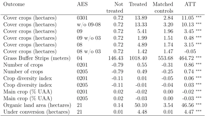
We implement DID-matching by comparing the before/after difference in practices for the treated to the similar difference for the untreated twins. We use 2000 as our before treatment date and 2005 as the after treatment date. If there exist fixed through time unobserved determinants that lead treated farmers to have persistently better practices than their untreated twins, comparing only the evolution of practices through time gets rid of this kind of selection bias. For example, the third column of table 3 shows that the average increment in the implantation of cover crops among all untreated farmers between 2000 and 2005 is 0.72 ha, while the corresponding estimate for treated farmers, whown in column 4, is 13.89 ha. Estimating the effect of AES 0301 by using a simple before/after comparison of the practices of the treated farmers would yield an estimate of the average causal effect of AES 0301 of 13.89 ha of additional implanted cover crops. But, as shown in column 5, untreated farmers have increased their area implanted in cover crops by 2.84 ha during the same period. The average causal effect of AES 0301 estimated by DID-matching is thus 11.05 ha.
This effect is 2 ha lower than the effect measured by simple matching and presented in table 2. This shows some evidence of selection bias due to unobserved variables. Before the AES was implemented, treated farmers already differed from their untreated twins. To calculate this difference, note that treated farmers implanted 17.24 ha of cover crops in 2005 (column 4 in table 2), which represents an increase of 13.89 ha relative to the area implanted in 2000 (column 4 in table 3). In 2000, treated farmers thus implanted 17.24-13.89=3.35 ha of cover crops in 2000. The same calculation for untreated farmers yields 4.19-2.84=1.35 ha of cover crops implanted in 2000. Thus, even before entering the AES, treated farmers implanted more cover crops (2 ha) than their untreated twins. We interpret this difference as selection bias due to unobservable variables (productivity, environmental preferences). If it is constant through time, we just have to decrease to difference in practices between treated farmers and their twins after the AES has been introduced presented in table 2 (13.05 ha) by 2 ha to get an estimate of the ATT of AES 0310. This correctly yields to the estimate of 11.05 ha presented in table 3.
To summarize this procedure, we have shown in table 2 that selection bias due to observables was estimated to be of 3 ha. In this section, we have estimated selection due to unobservables to be of 2 ha. Thus, total selection bias that shows up when comparing treated farmers to all untreated farmers is estimated to be of 5 ha of cover crops, which is sizable. The time trend bias for this AES has also been estimated to be of 2.84 ha (the
average increase in practices for the untreated twins).
Finally, we can estimate the total windfall effect allowing for selection on both observ-ables and unobservobserv-ables. Farmers benefiting from AES 0301 implant 17.24 ha of cover crops in 2005 and receive payments compensating them for doing so on this area. The causal effect of AES 0301 as estimated by DID-matching is 11.05 ha. The total windfall effect is the area that treated farmers would have implanted in the absence of the AES: 17.24-11.05=6.19 ha. It can also be calculated as the sum of the area implanted by their untreated twins in 2005 (4.19 ha) and the difference in implanted area between treated farmers and their untreated twins in 2000 (2 ha).
Table 3: Average causal effects of AES measures estimated by DID-matching Outcome AES Not Treated Matched ATT
treated controls
Cover crops (hectares) 0301 0.72 13.89 2.84 11.05 ∗∗∗
Cover crops (hectares) w/o 09-08 0.72 13.33 3.20 10.13 ∗∗∗
Cover crops (hectares) 09 0.72 5.41 1.96 3.45 ∗∗∗
Cover crops (hectares) 09 w/o 03 0.72 1.99 1.51 0.48 ∗∗∗
Cover crops (hectares) 08 0.72 4.89 1.74 3.15 ∗∗∗
Cover crops (hectares) 08 w/o 03 0.72 1.42 1.47 -0.05 Grass Buffer Strips (meters) 04 146.43 1018.40 553.68 464.72 ∗∗∗
Number of crops 0201 -0.79 0.55 -0.31 0.86 ∗∗∗
Number of crops 0205 -0.79 0.49 -0.25 0.74 ∗∗∗
Crop diversity index 0201 -0.11 0.01 -0.05 0.06 ∗∗∗
Crop diversity index 0205 -0.11 -0.01 -0.04 0.03 ∗∗∗
Main crop (% UAA) 0201 0.02 -0.02 0.00 -0.02 ∗∗∗
Main crop (% UAA) 0205 0.02 -0.03 0.00 -0.03 ∗∗∗
Organic land area (hectares) 21 0.14 50.10 3.54 46.56 ∗∗∗
Under conversion (hectares) 21 0.01 4.48 0.01 4.47 ∗∗∗
Note: the ATT is the Average Treatment Effect on the Treated. It is estimated using the nearest neighbor DID-matching, except for AES 04 and 21 for which simple matching is used because corresponding outcomes were not measured in the 2000 census. UAA refers to Usable Agricultural Area. stars indicate the statistical confidence level with which the null of no treatment effect can
be rejected: ∗∗∗, ∗∗ and∗respectively stand for 1%, 5% and 10%.
The estimated treatment effects are contrasted, as are estimates of selection bias. Treatment effects estimated for cover crops implantation (AES 0301) are large: an in-crease in 11 ha of implanted cover crops per treated farm. This translates into an inin-crease of almost 110 000 ha of cover crops overall. This nevertheless is roughly equal to half of the area subsidized, implying that windfall effects are equal to half of the subsidized area.
Windfall effects are even larger in the case of crop diversity AES: even though the number of crops has increased by a little less than one, meaning that an additional crop has been added to the rotation thanks to the AES, crop diversity measured by an index of evenness has increased only slightly: the index has increased by .03 to .05 while its mean is .8 for the treated (see Table 2). This is explained by the very tiny reduction in the area dedicated to the main crop in the rotation: as requested by the requirements of these AES, a new crop has been added to the rotation, but on a very limited area, limiting the scope of the impact of the AES.
Our results suggest that the size of windfall effects of the AES programs depends on the specific prerequisites for each AES. For example, the AES supporting conversion to organic farming, which combined large payments with the strong requirement of not being an organic farmer when applying for the AES, have had negligible windfall effects. We estimate that almost 90 % of the near doubling of area dedicated to organic farming that occurred between 2000 and 2005 in France is due to the AES 21.
5.3
Cost benefit analysis of individual AES
Estimating average causal effects is a very important necessary step in the evaluation of public policies, but it has to be included in a fully-fledged welfare analysis to enable a com-plete evaluation of a policy (Heckman, LaLonde, and Smith, 1999). Economists generally use a cost-benefit criterion to evaluate environmental policies (Bockstael and Freeman, 2005). To our knowledge, there has been very little work bringing together causal analysis and cost-benefit analysis in environmental economics. The main challenge in environmen-tal economics is the monetary valuation of the alterations to the environment causally attributable to the policies. In labor economics, as outcomes are monetary measures as income, integration of estimates of treatment effects in a cost benefit analysis is more natural, but even in this case, estimation of average causal effects is not sufficient for complete cost-benefit evaluation and may not be necessary for some more general welfare criterion sensitive to distributional issues (Heckman and Smith, 1998; Dehejia, 2005).
The main challenge in our case is to give a monetary value to changes in agricultural practices. This entails first being able to understand how changes in agricultural practices affect the environment, second understanding how these environmental changes affect in-dividuals’ utility (maybe through changes in their health) and third giving a monetary value to these utility changes (Bockstael and Freeman, 2005). It is not sure that changes in average practices is the relevant information to be able to back out changes in envi-ronmental quality. There are indeed issues with the spatial distribution of these changes (maybe changes of individual practices scattered across a given area are less efficient at improving environment quality than changes located in one specific spot).
Putting these important issues aside, how could we use the estimates of the average causal effects in a cost-benefit analysis? Let’s suppose that social benefits from a given agricultural practice are proportional to the total area where this practice is implemented. The per hectare monetary social benefit from the practice is thus assumed to be constant and equal to Bh. A cost-benefit analysis of a given AES entails comparing the total
benefit the AES yields when implemented to its cost and to the total benefit that would have been reached had the AES not been implemented. Under the assumption that untreated farmers have not changed their practices because of the implementation of the AES scheme, cost benefit analysis can focus only on treated farms. For the average treated farm, the total benefit generated under the scheme is the total area under the practice multiplied by Bh: E [Y1|D = 1] Bh, where E [Y1|D = 1] is the area under the practice in
the average treated farm when it receives treatment. We consider only the direct costs of the program, i.e. direct payments to farmers. We thus disregard administrative costs, deadweight losses due to taxation and profit loss to the farmer due to the implementation of the AES. Costs are thus per hectare payments (Ch) multiplied by total area under
the AES on the farm: E [Y1|D = 1] Ch. When the treatment is implemented, the net
benefit is thus: E [Y1|D = 1] (Bh − Ch). This has to be compared with the benefit that
E [Y0|D = 1] is the counterfactual, i.e. the area under the practice that would have been
observed in the average treated farm had the program not been implemented. The cost benefit criterion for the average treated farm is thus:
CB = E [Y1|D = 1] (Bh− Ch) − E [Y0|D = 1] Bh (1) = E [Y1 − Y0|D = 1] | {z } AT T Bh− E [Y1|D = 1] Ch (2) = AT T (Bh− Ch) − E [Y0|D = 1] | {z } W Ch, (3)
where AT T stand for average causal effect of the treatment on the treated farms and W is the windfall effect.8
Cost benefit analysis of the AES thus crucially relies on the extent of additionality (AT T ) vs windfall effects (W ). Under the AES, farmers receive a payment for all the area under the practice, not for the additional area they have implanted because of the AES. They thus receive a payment for practices they would have adopted in the absence of the AES, which leaves scope for windfall effects: had the AES not been implemented, farmers may have nonetheless adopted the practice because they have other incentives for doing so.
The results of section 5 gives us both the ATT and the counterfactual level of prac-tices (W ). Ch can be recovered from per hectare payments of the individual AES. The
crucial parameter lacking is thus the per hectare social benefit of implementing the AES, Bh. It is very complex to come up with such a number. In order to do so, we must
be able to delineate all the environmental consequences of a given change in practices and to give them a monetary value. For example, implanting cover crops may prevent nitrogen runoff, which in turn may decrease the amount of nitrogen in ground water. This may increase biodiversity, which may be valued per se, and also decrease nitrogen concentration in drinking water, which may result in reduced prevalence of cancer, for example. van Grinsven, Rabl, and de Kok (2010) estimate a social cost of 0.7 eper kg of nitrate-N runoff from fertilizer usage. It remains to be determined how many kg of nitrate-N per hectare can be avoided by implanting a cover crop. In this paper, we do not take a stand on the social value of a given agricultural practice. We instead calculate a lower bound on this social value above which the benefits of the AES exceed its costs. This lower bound B∗
h can be defined from equation (3):
B∗ h =
AT T + W
AT T Ch. (4)
From equation (4), we can see that a higher AT T leads to a lower bound (the AES has a positive social benefit even if the social benefit of the practice is moderate), a larger W leads to a higher bound. When there is no windfall effect, the bound is equal to the direct cost of the AES. Table 4 present estimates of the bound for AES 0301, 04 and 21. Estimating such a bound for AES 02 is more intricate, since the link between payments, outcomes and social benefit is more complex.
From table 4, we can see that the size of windfall effects relative to additional effects
8
The last equality comes from the fact that observed practices in the presence of the AES are equal
to practices in the absence of the AES and the causal effect of having the AES (Y1= Y1− Y0+ Y0) and
Table 4: Cost-benefit analysis of various AES
AES Corresponding practice ATT W Ch (e/ha) B∗h (e/ha)
0301 Implanting cover crops (ha) 11.05 6.19 70 109 04 Implanting grass buffer strips (km) 0.46 0.56 110 244 21 Conversion to organic farming (ha) 50.10 3.54 244 261
Note: the ATT is the Average Treatment Effect on the Treated. It is taken from table 3. W is the windfall effect, estimated by taking the difference between the average area under the
practice in 2005 for the treated (column 4 in table2) and the ATT. Ch is the payment per
hectare received by farmers taking the AES. B∗
h is the lower bound on the social benefit from
one hectare under the practice that makes the AES socially beneficial. Is is calculated according to equation (4).
is indeed crucial. Windfall effects are larger than additional effects for AES 04, meaning that the social value of an additional implanted hectare of grass buffer strips has to be superior to twice the cost per hectare of the AES to ensure that the AES has a positive social benefit. The estimated lower bound for the AES 04 is indeed 244 e/ha of implanted grass buffer strip, which is compatible with realistic estimates of the social value of this practice. (Lankoski and Ollikainen, 2003) estimate the social cost of nitrogen runoff to be of 1.6 e/kg of N-fertilizer. One hectare of grass buffer strip would thus have to prevent the runoff of 144 kg of N-fertilizer to be cost-efficient. This calculation disregards potential benefits of grass buffer strips other than preventing nitrogen runoff, as preventing pesticide runoff and increasing biodiversity. Despite its large windfall effects, AES 04 could thus very well be cost effective.
Windfall effects are lower for AES 0301, which translates into a lower lower bound on the cost effectiveness of the scheme: one hectare of cover crops have to prevent 109 eof social cost to be cost-efficient. van Grinsven, Rabl, and de Kok (2010) estimate that the social cost of one kg of N-fertilizer leaching into groundwater is equal to 1e, mainly because of an increase in cancer prevalence. To ensure that AES 0301 is cost effective, implanting one hectare of cover crop should prevent the leaching of 109 kg of N-fertilizer, which does not seem realistic. On the other hand, cover crops or reduced nitrogen leaching may have other benefits, for example in terms of biodiversity or reduced erosion.
Windfall effects are extremely small for AES 21. This translates in a lower bound for cost-effectiveness (261 e) very close to the per hectare payment (244 e), which is in line with results in Sandhu, Wratten, Cullen, and Case (2008) on the social value of organic farming compared to conventional farming.
Overall, we think that the main advantage of causal analysis is that it provides some key ingredients to cost-benefit analysis. It obviously does not enable to perform a com-plete cost-benefit analysis, but can provide very interesting results when combined with adequate supplementary data on the social value of the subsidized practices.
6
Directions for further research
In this section, we discuss the possibility of extending the methods we use to evaluating the effects of changes in some parameters of the schemes. Second, we discuss the merits of experimental evaluations of the AES.
6.1
Evaluating schemes promoting extensive herding
Measures promoting extensive herding account for the largest share of the budget for the AES in France. Unfortunately, we cannot conclude on the extent of additional and windfall effects for payments for extensive herding, because we find evidence of violations of the identifying assumptions of DID-matching for these AES. Indeed, almost all eligible farmers took this AES, meaning that very few twins can be found for the treated. The ones we find experience a really strong decrease in their usable agricultural area (UAA) while at the same time the treated experience an increase by the same amount in their UAA. This signals a transfer of land between treated and untreated twin farmers that has taken place because of the AES or signals an unobserved difference in farm dynamics between treated and untreated that our method cannot control for. Either explanation leads to biased inference by DID-matching. In section 6.3, we discuss how experimental methods could help solving this problem.
6.2
Simulating the effect of altering parameters of the AES
In the previous analysis, we have considered each AES separately and have implicitly assumed that each AES was the only means of altering a given agricultural practice. This seems correct for AES 0301, 04, and 21, but is not true for AES 0201 and 0205: they both tend to alter the same set of practices. It could be interesting to compare the social value of implementing both AES simultaneously with the social value of implementing only one of them (for example, only AES 0205). In this latter case, the farmers that would have implemented AES 0201 could either take AES 0205 or no AES. To perform such an evaluation, we would thus have to predict the choice of the farmers normally choosing AES 0201 and to estimate the causal effect that AES 0205 has on them. We are currently investigating the possibility of performing such an analysis by extending the matching methods.A second type of extension would entail predicting the effect of alterations in the price and the requirements of a given AES. Since the characteristics do not vary in our sample because unit payments and requirements are almost identical for identical farmers, it would be very difficult to predict the consequences of such changes using only the data generated by the 2000-2006 program.
A third type of extension would be to consider alternative allocation mechanisms of the payments for the AES. The French AES are allocated under a uniform payment mechanism: all farmers entering an AES are roughly paid the same amount per hectare of agricultural practice subsidized. This leaves a lot of scope for windfall effects: farm-ers with zero or small costs of complying with the AES requirements receive the same compensation as farmers with high costs of coping with the requirements. One way of mitigating these effects is to condition entry and/or payment on farm characteristics that proxy costs (payments for grass buffer strips differ across technico-ecnonomic orientations, farmers that converted to organic farming before the AES was in place are excluded from payments), but there remains room for windfall effects even after conditioning on these observed characteristics. One way to reduce the windfall effects and to improve the cost effectiveness of an AES program is to auction it: given a set of constraints on prac-tices, farmers bid on the per hectare price and the area on which they are willing to implement the constraints. Payments are allocated starting from the lowest bid until the total budget for the AES has been spent. Auctions are theoretically more efficient than unique payments to allocate payments for AES because payments to farmers are closer
to their unit costs of delivering the service, which decreases windfall effects. This in turn saves money that enables paying farmers with costs higher than the uniform payment for providing the service. Auctions thus achieve a larger area under the AES for the same budget. Evaluating this alternative form of payment is very difficult with data coming from the implementation of unique payments only, and it would require making heroic assumptions.
In the next section, we investigate how the use of randomized control trials could help making progress along these two dimensions: evaluating the effects of variations in prices and requirements of a given AES and comparing various ways of implementing an AES, for example auctions and a unique payment scheme.
6.3
Experimental evaluation of AES and alternative allocation
mechanisms
Indeed, an important area for further research is the implementation of evaluation meth-ods based on randomized control trials (RCT) to estimate the causal effects of AES, or of different ways of implementing AES. RCTs are based on a very simple intuition: if treated farmers are selected at random, the direct comparison of their practices to the ones of the untreated farmers gives the average causal effect of the AES (Burtless, 1995; Duflo, Glennerster, and Kremer, 2007). The validity of an RCT requires that random-ization is performed among a sufficiently large group of farmers, so that the law of large number ensures that treated and untreated farmers are ex ante identical. It also requires the assumption that the practices of untreated farmers are not altered by the presence of the treatment. This assumption is also required for the methods developed in this paper. Because this is not likely to hold for some applications, we discuss some ways to relax this assumption. Finally, to ensure the policy relevance of the results of a RCT, we need to assume that it has not disrupted the way the program normally operates. For example, the selection of the beneficiaries and their behavior may be altered by randomization (Heckman and Smith, 1995).
The main advantages of RCTs are that they do not require assumptions on the form of selection bias, as the ones we needed to ensure that DID-matching is unbiased. Coun-terbalancing this, political constraints are often raised against RCTs, because they entail randomly denying the benefit of the program to a subsample of the population that would like to enter it. In the case of AES, we think that this problem might be alleviated if we confine RCTs to the evaluation of new types of AES vs more traditional types, rather than evaluating these AES vs no AES. Another way of mitigating this issue is to ran-domize an encouragement to participate in a given AES (receiving a letter explaining the merits of the AES, for example), while allowing everyone to enter each scheme. The policy-relevance of the evaluation is nevertheless reduced because we can only estimate the effect of the scheme on those that have been encouraged to enter it, which might be a small portion of the overall treated population.
It is possible to study the effects of varying both the price and the requirements of a given AES by randomly allocating the possibility of accessing the different options, for example across space. For example, AES 0205 could be implemented everywhere, but the possibility of opting for AES 0201 could be limited to a random subset of zones. We could thus estimate the additional effect of proposing AES 0201.
Another possibility would be to offer the possibility to enter an AES dedicated to extensive herding more stringent than the current one on a random subset of areas. This
would prevent all farmers that would benefit from this more stringent version of entering it and thus being unable to estimate its effect. We could study the diffusion and price effects of this new scheme by comparing untreated areas located close to the treated areas to the ones located further away, as in (Miguel and Kremer, 2004).
Finally, by implementing auctions to allocate payments for AES on a random subset of places, while maintaining unique payments on the other zones, we could test whether the theoretical superiority of auctions has empirical content.
7
Conclusion
The results we obtain point at positive but contrasted results of the AES we study. AES with strong prerequisites limiting the extent of windfall effects as the ones directed to organic farming have had a very large impact, nearly doubling the area dedicated to organic faming in France over the period of study. On the contrary, AES aiming at increasing crop diversity have had mixed results, with large selection bias and and low causal effects, because their loose prerequisites enable entry by farmers having highly diverse rotations in the absence of the AES. We give a first tentative cost-benefit analysis of certain AES. We show that large windfall effects can be compensated by large social benefits.
We make some suggestions aiming at improving the evaluation of future programs. We argue that evaluation should be prepared at the same time the program is designed. This would improve the collection of data and enable using the first results of the evaluation to design the next program (by suppressing or altering the less efficient AES). Finally, this could allow for the implementation of experimental methods to evaluate policies that do not comply with the assumptions of DID-matching, like payments for extensive herding. One very interesting direction for further research could be to compare how auctioning the AES could compare in terms of windfall effects. Experimental methods selecting randomly areas in which auctions or traditional uniform payment scheme are implemented would allow a robust comparison of these two approaches.
References
AND (2008): “Évaluation ex-post du PDRN: Partie sur le "soutien à l’agro environ-nement",” Rapport d’évaluation, Ministère de l’Agriculture et de la Pêche.
Bockstael, N. E., and A. M. I. Freeman (2005): “Welfare Theory and Valuation,”
in Handbook of Environmental Economics, ed. by K.-G. Mäler,and J. R. Vincent, vol.
2: Valuing Environmental Changes of Handbook of Economics, chap. 12, pp. 517 – 570. Elsevier.
Burtless, G. (1995): “The Case for Randomized Field Trials in Economic and Policy Research,” Journal of Economic Perspectives, 9(2), 63–84.
Chabé-Ferret, S., and J. Subervie (2009): “Evaluation de l’Effet
Propre des Mesures Agro-Environnementales du PDRN 2000-2006 sur les Pratiques des Agriculteurs,” Rapport d’évaluation, Cemagref,
(2010): “Estimating the Impact of the French AgroEnvironmental Schemes on Agricultural Practices by Difference-In-Difference Matching : Theoretical Justification, Robustness Tests and Application to a French Program,” in 4th World Congress of Environmental and Resource Economists (WCERE), Montreal, Canada.
Dehejia, R. H.(2005): “Program Evaluation as a Decision Problem,” Journal of Econo-metrics, 125(1-2), 141–173.
Duflo, E., R. Glennerster, and M. Kremer(2007): “Using Randomization in
De-velopment Economics Research: A Toolkit,” in Handbook of DeDe-velopment Economics, ed. by T. P. Schultz,and J. A. Strauss, vol. 4, chap. 61, pp. 3895–3962. Elsevier.
Hazeu, G., B. Elbersen, C. van Diepen, B. Baruth, and M. Metzger (2006):
“Regional typologies of ecological and biophysical context,” Discussion paper, System for Environmental and Agricultural Modelling Linking European Science and Society (SEAMLESS).
Heckman, J. J., H. Ichimura,andP. E. Todd(1997): “Matching as an Econometric
Evaluation Estimator: Evidence from Evaluating a Job Training Programme,” The Review of Economic Studies, 64(4, Special Issue: Evaluation of Training and Other Social Programmes), 605–654.
Heckman, J. J., R. J. LaLonde, and J. A. Smith (1999): “The Economics and
Econometrics of Active Labor Market Programs,” in Handbook of Labor Economics, ed. by O. C. Ashenfelter,and D. Card, vol. 3, chap. 31, pp. 1865–2097. Elsevier, North
Holland.
Heckman, J. J., and J. Smith (1995): “Assessing the Case for Social Experiments,”
Journal of Economic Perspectives, 9(2), 85–110.
(1998): “Evaluating the Welfare State,” in Econometrics and Economics in the 20th Century, ed. by S. Strom. Cambridge University Press, New York.
Imbens, G. W.(2004): “Nonparametric Estimation of Average Treatment Effects Under Exogeneity: A Review,” The Review of Economics and Statistics, 86(1), 4–29.
Jones, R. J. A., R. Hiederer, E. Rusco, and L. Montanarella (2005):
“Esti-mating Organic Carbon in the Soils of Europe for Policy Support,” European Journal of Soil Science, 56(5), 655–671.
Lankoski, J., and M. Ollikainen (2003): “Agri-Environmental Externalities: a
Framework for Designing Targeted Policies,” European Review of Agricultural Eco-nomics, 30(1), 51–75.
Metzger, M. J., R. G. H. Bunce, R. H. G. Jongman, C. A. Mücher, and J. W.
Watkins (2005): “A Climatic Stratification of the Environment of Europe,” Global Ecology & Biogeography, 14(6), 549–563.
Miguel, E., and M. Kremer (2004): “Worms: Identifying Impacts on Education and
Pufahl, A., and C. R. Weiss (2009): “Evaluating the Effects of Farm Programmes:
Results from Propensity Score Matching,” European Review of Agricultural Economics, 36(1), 79–101.
Sandhu, H. S., S. D. Wratten, R. Cullen, and B. Case (2008): “The Future of
Farming: The Value of Ecosystem Services in Conventional and Organic Arable Land. An Experimental Approach,” Ecological Economics, 64(4), 835 – 848.
van Grinsven, H., A. Rabl, and T. de Kok (2010): “Estimation of Incidence and
Social Cost of Colon Cancer due to Nitrate in Drinking Water in the EU: a Tentative Cost-Benefit Assessment,” Environmental Health, 9(1), 58.