Analytical solution to a simplified circulatory model using piecewise linear elastance function

Analytical Solution to a Simplified Circulatory

Model using Piecewise Linear Elastance Function

by

Jinn Jiau Spenser Chen

B.Eng., Electrical and Electronic Engineering (2002)

Imperial College London

Submitted to the Department of Electrical Engineering and Computer

Science

in partial fulfillment of the requirements for the degree of

Master of Science in Electrical Engineering and Computer Science

at the

MASSACHUSETTS INSTITUTE OF TECHNOLOGY

September 2003

©

Jinn Jiau Spenser Chen, MMIII. All rights reserved.

The author hereby grants to MIT permission to reproduce and

distribute publicly paper and electronic copies of this thesis document

in whole or in part.

A uthor ...

Department of Electrical Engineering and Computer Science

July 13, 2003

Certified by...

....

George C. Verghese

--,Professor of Electrical Engineering

ksis

'pervisor

Accepted by...

...

Arthur C. Smith

Chairman, Department Committee on Graduate Students

MASSACHUSETTS INSTITUTE OF TECHNOLOGY

Analytical Solution to a Simplified Circulatory Model using

Piecewise Linear Elastance Function

by

Jinn Jiau Spenser Chen

Submitted to the Department of Electrical Engineering and Computer Science

on July 13, 2003, in partial fulfillment of the

requirements for the degree of

Master of Science in Electrical Engineering and Computer Science

Abstract

Due to the strong analogy between electrical circuits and fluid systems, circuit-based lumped parameter representations of the hemodynamic system are commonly used in teaching and research to analyze the system-level behavior of the circulation over time scales of a few to a few hundred beats. While efficient numerical methods exist for integration of the governing differential equations, we present an analytical solution of the pressure (voltage) waveforms in a simplified time-varying elastance model, or pulsatile heart model. The pumping action of the heart is captured by the ventricular compartment, which is primarily made up of a time-varying capacitor. We define the time-varying capacitance as the inverse of a piecewise linear elastance function that is a close fit to population-averaged hemodynamic data. The analytical solution provides an explicit mathematical description of the circuit model dynamics without the need for a numerical solver to integrate the differential equations, thereby reducing computational complexity. A comparison of the analytical solution against a numerical simulation of the pulsatile model in terms of steady-state and transient responses showed that the maximum relative error is no more than 1.79% across the waveforms. Moreover, it allows for the representation of the pressure waveforms by a set of discrete-time points per cycle, which we term the discrete-time analytical solution, without any loss of information. The discrete-time analytical solution is shown to reduce the simulation time of the pulsatile model by a factor of 5000. The analytical solution can potentially aid in developing procedures for estimating model parameters. Extension of the approach outlined above to a dual chamber heart and more elaborate peripheral circulatory model will constitute worthwhile directions for further work.

Thesis Supervisor: George C. Verghese Title: Professor of Electrical Engineering Associate Supervisor: Thomas Heldt

Acknowledgments

First, I would like to thank my thesis advisor, Professor George Verghese, for all his invaluable help and patient guidance throughout the last year. He was always available to guide me through the problems I encountered in the project, and to offer advice on classes and life in MIT, which helped me settle down quickly into a new environment here, having come from Imperial College in London. His insight, experience and enthusiasm helped make this project possible.

Special thanks to Thomas Heldt who was always there to answer my questions and I am grateful to him for all the help he rendered me with thesis writing, Latex and C programming among many other things. In addition, I would like to thank Professor Roger Mark for giving me the opportunity to work in the Laboratory for Computational Physiology, where I had the chance to work with a group of brilliant and highly motivated students and researchers.

I would also like to express my gratitude to the Singapore Armed Forces for their

financial support over the past four years, without which none of these would be possible.

Finally but most importantly, special thanks to my parents, my sister and all the friends I have made here for their unwavering support and encouragement throughout my time here at MIT.

Contents

1 Introduction

1.1 Computational Modeling . . . .

1.2 Background . . . . 1.2.1 The Computational Hemodynamic Model 1.2.2 Piecewise Linear Elastance . . . .

1.3 Problem Motivation . . . . 1.4 Goals and Outline . . . .

2 Pulsatile Model with Piecewise Linear Elastance

2.1 Pulsatile Model . . . . 2.2 Simulation in HSPICE . . . .

3 Deriving the Analytical Solution 3.1 Dividing into Subproblems . . .

3.1.1 Notation . . . . 3.1.2 Approach Outline . . 3.1.3 Region I . . . . 3.1.4 Region II . . . . 3.1.5 Region III . . . . 3.1.6 Region IV . . . . 3.1.7 Region V . . . . 3.1.8 Region VI . . . . 3.1.9 Region VII . . . . 13 14 15 17 19 21 23 25 25 27 31 31 33 33 34 36 38 41 41 43 45 . . . . . . . . . . . . . . . . . . . . . . . .

3.1.10 Initializing the Next Cycle . . . . 46

3.2 Implementing the Analytical Solution . . . . 48

3.2.1 MATLAB . . . . 48

3.2.2 C Programming Language . . . . 48

3.3 Discrete-time Analytical Solution . . . . 50

4 Comparison of Simulations ₅₃ 4.1 Comparison of Steady-state Numerics . . . . 54

4.2 Comparison of Dynamic Responses . . . . 57

4.2.1 Changes in R3 . . . . 57

4.2.2 _{Changes in T . . . . 60}

4.3 Computational Efficiency . . . . 64

5 Extension Work ₆₅ 5.1 Model Parameter Sensitivity . . . . 65

5.2 Elastance Parameter Estimation . . . . 67

6 Conclusion ₇₁ A Mathematical Working ₇₃ A.1 Deriving V2 1(t) . . . . 73 A.2 Deriving Qh3(t) . . . . 75 A.3 Deriving Qh6(t) . . . . 77 A.4 Deriving Qh7(t) . . . . 78 B Program Codes 79 B.1 Analytical Solution in MATLAB . . . . 79

B.2 Analytical Solution in C . . . . 86

B.3 Discrete-time Analytical Solution in C . . . . 96

Bibliography ₁₀₅

List of Figures

1-1 The human heart [13] ... . 14

1-2 Circuit-based hemodynamic model

[4]

. . . .

18

1-3 Piecewise linear elastance function vs. experimental elastance data [12] of the left ventricle over 1 cardiac cycle . . . . 20

2-1 Simplified three-compartment circulatory model . . . . 26

2-2 HSPICE simulation output of the pulsatile model using piecewise linear elastance . . . . 29

3-1 Steady-state voltage waveforms (top) and piecewise linear elastance function (bottom) divided into seven regions over 1 cycle . . . . 32 3-2 Equivalent circuit model for Region I . . . . 34

3-3 Equivalent circuit model for Region II . . . . 36

3-4 a) Equivalent circuit model for Region III b) Modified circuit model

(R

38

3-5 Plot of function f(t) and the constant approximation c . . . . 40

3-6 Plot of function g(t) and the linear approximation h(t) . . . . 44

3-7 Voltage waveforms generated by the analytical solution in MATLAB . 49

3-8 Voltage waveforms generated by the analytical solution in C . . . . . 49

3-9 Representation of full voltage waveforms by discrete-time points over 1 cycle (top); discrete-time voltage waveforms (bottom) . . . . 51

4-1 Steady-state voltage waveforms generated by circuit simulation (top) and analytical solution (bottom) of the pulsatile model . . . . 55

4-2 Comparison of steady-state dynamics of V (top), V2 (middle) and Vh

(bottom ) . . . . 56

4-3 Transient responses of circuit simulation (top) and analytical solution (bottom) of the pulsatile model to changes in R3 . . . . . . . . 58

4-4 Comparison of transient dynamics of V (top), V2 (middle) and Vh

(bottom) due to changes in R3 . . . . . . . . 59

4-5 Transient responses of circuit simulation (top) and analytical solution (bottom) of the pulsatile model to changes in T . . . . 62

4-6 Comparison of transient responses of V (top), V2 (middle) and Vh

(bottom) to changes in T . . . . 63

List of Tables

1.1 Analogy of physiological and electrical variables .

2.1 System parameters . . . .

3.1 Definition of the 7 regions . . . .

4.1 4.2 4.3 4.4 4.5

Characteristic variables of voltage waveforms . . . .

Comparison of steady-state responses . . . . Comparison of transient responses to changes in R3

Comparison of transient responses to changes in T . Comparison of CPU times . . . .

5.1 Numerical sensitivity analysis of model parameters

17 27 32 . . . . 53 . . . . 54 . . . . 58 . . . . 60

. . . .

64

Chapter 1

Introduction

The human circulatory or cardiovascular system circulates blood around the body, in order to deliver oxygen and nutrients to all parts of the body and to remove metabolic waste products; it also plays an important role in the functioning of the immune system. The human cardiovascular system consists of two structurally dis-tinct components: the heart, which is a muscular pump, and the blood vessels in which the blood flows.

There are three varieties of blood vessels: arteries, veins and capillaries. The arteries carry blood away from the heart. The capillaries are very thin vessels where the actual oxygen and nutrient exchange takes place, and which form the interface between arteries and veins. Finally, the veins carry the blood back to the heart. The arterial system is characterized by high resistance and low capacitance, while the venous system has low resistive and high capacitive properties.

Figure 1-1 shows a schematic drawing of the human heart [13]. The heart is primarily a muscular shell. There are four chambers inside the heart that fill with blood. Two of these chambers, the atria, form the curved top of the heart, while the other two, called ventricles, meet at the bottom of the heart to form a pointed base. The left and right sides of the heart each houses one atrium and one ventricle, with a valve connecting the atrium to the ventricle below it. De-oxygenated blood returning from the body enters the heart in the right atrium. From the right atrium, the blood passes through the tricuspid valve to enter the right ventricle. The blood is

then pumped into the pulmonary arteries, passing the pulmonary valve, from where it goes to the lungs. After becoming oxygenated in the lung's capillaries, the blood is carried by the pulmonary veins to the left atrium. It then passes through the bicuspid or mitral valve into the left ventricle, from where it is pumped into the aorta through the aortic valve. The aorta branches into smaller and smaller arteries that finally lead to capillary beds in the tissue. Here oxygen is exchanged for carbon dioxide. The blood eventually empties back into the right atrium via veins which join into the inferior vena cava (veins coming from the lower body) and superior vena cava (from

the upper body).

Superior

\kma cava

ulmona y

Artery

Figure 1-1: The human heart [13]

1.1

Computational Modeling

Computational models are widely used by engineers and researchers as quantitative representations of physical and non-physical systems for simulation studies. Presently,

many computational models of the human body systems are becoming rapidly avail-able as biomedical engineering researchers combine knowledge of the human anatomy with the processing power of modern computers to construct simulations of the human organs. Computational modeling and simulation studies can facilitate the advance-ment of biomedical research through the design and testing of new therapeutics, including medical devices, pharmaceuticals and clinical procedures, because these models, particularly of the heart, can accurately predict and simulate system re-sponses to perturbations in physiological conditions at the molecular, cellular and organ levels. Moreover, computational modeling in cardiovascular research offers a more cost-effective alternative to clinical testing, which often involves highly invasive measurement procedures that are both expensive and time-consuming.

As described earlier, the human circulatory system is a highly complex and dy-namic system, which requires the interaction and independent functioning of the heart, pulmonary circulation and systemic circulation to ensure its own proper func-tioning. Despite the complexity, biomedical engineering researchers have developed computational models of the circulatory system, capable of simulating cardiovascular dynamics over a broad range of biological levels and time scales, from molecular to organ level and from a single heartbeat to several thousand cardiac cycles.

1.2

Background

Due to the strong analogy between electrical circuits and fluid systems, electrical models are widely used in computational modeling of the cardiovascular system. In general, for a closed fluid system, there is an electrical circuit whose behavior is iden-tical (up to conversion factors). Pressure differences in the circulatory system are created by the pumping action of the heart, which moves the blood from a region of high pressure to a region of low pressure. Similarly, electric current flows from regions of high potential to regions of low potential and is impeded by circuit resis-tances. Thus, in an electrical analog of the cardiovascular system, blood flow would map to electric current, pressure differences to voltage, and flow resistance to ohmic

resistance.

At the organ level, description of the heart as a pump has been dominated by mod-els based on a time-varying ventricular elastance, or its inverse, compliance. Elastance is a measure of chamber stiffness and thus ventricular elastance is a measure of the contractile state of the heart. The time-varying elastance-based ventricle models have proven to be useful representations of the right and left heart, and when coupled to appropriate models of the pulmonary and systemic circulations, allow for simulation of realistic pulsatile pressure and flow waveforms.

The classical definition of (incremental) elastance E, relates a true differential volume

&U

&P:

E = (1.1)

In defining ventricular elastance, Suga (1969) opted for the definition of elastance as the ratio of ventricular volume and pressure:

P(t )

E(t) = (1.2)

U(t)

where E(t), P(t) and U(t) represent the instantaneous elastance, pressure and volume respectively at time t. More precisely,

P(t) P(t)

U(t) - Uo Ud(t)

-> Ud(t) = (1.4)

E(t)

where U0 denotes the zero-pressure volume, and Ud(t) denotes the distending volume.

A description of the charge Q(t) on a capacitor with capacitance C(t) and potential

difference V(t) in an electrical circuit is given by:

Q(t)

=

C(t)V(t)

(1.5)

Clearly, an analogy exists between Equation 1.4 and 1.5, where electric charge corre-sponds to distending blood volume, and elastance to the inverse of capacitance. Table

1.1 shows the correspondence between physiological and electrical elements that we

have identified thus far.

Physiological Electrical

pressure P [mmHg] voltage V [V]

flow F [ml/min] current I [A] flow resistance R [mmHg - min/ml] ohmic resistance R

[Q]

compliance C [ml/mmHg] capacitance C [F]

elastance E [mmHg/ml] elastance E [F-1]

volume U [ml] charge

Q

[C]

Table 1.1: Analogy of physiological and electrical variables

Based on these relations, several electrical models of the cardiovascular system have been constructed in order to produce and analyze hemodynamic waveforms in a controlled setting. In the next section, we will look at a circuit-based, lumped parameter model of the human circulatory system, which has been developed by Davis [4] to simulate short-term transient and steady-state hemodynamic responses to various physiological conditions.

1.2.1

The Computational Hemodynamic Model

Figure 1-2 shows a closed-loop lumped parameter hemodynamic model that is math-ematically formulated in terms of an electric analog model. The model consists of six compartments, each of which is made up of linear resistors, ideal diodes, volt-age sources and/or capacitors that can be linear or nonlinear, and time-invariant or time-varying.

The pumping action of the heart is realized by the time-varying capacitors, which represent the time-varying compliances of the right and left ventricles. The diodes are in place to ensure unidirectional current flow, just as valves in the heart ensure unidirectional flow of blood through the ventricles and parts of the venous system.

A time-varying voltage source simulates the changing transmural pressure across the

intrathoracic pressure variations, and assumes a simple sinusoidal function in the model.

Pulmonary Circulation

Systemic Circulation

Figure 1-2: Circuit-based hemodynamic model [4]

A more detailed discussion on the model components, as well as assignment of

parameter values, is given by Davis [4] and Heldt [6]. In summary, the model is a lumped parameter representation of the human circulatory system, without the feedback control loops to model arterial and cardiopulmonary baroreflexes. The heart is described using time-varying ventricular compliance models, which are primarily made up of time-varying capacitors.

1.2.2

Piecewise Linear Elastance

While there is no formal specification of the time-varying elastance, several reason-able choices have been suggested and used in hemodynamic models. Warner (1959) appears to have been the first to adopt a compliance description for a dynamic heart, in which he assigned one compliance value during diastole and another smaller value during systole. As a result, the ventricle is analogous to an elastic bag that becomes stiffer in systole, thereby producing an increase in ventricular pressure over this time period. Defares et al. (1963) avoided the stepwise transitions between diastolic and systolic compliance values by making elastance a continuously varying function of time. Today, computational models of the cardiovascular system assume a host of definitions of the ventricular elastance, including Warner's "2-state" compliance func-tion, which is widely used for its simplicity.

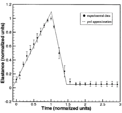
Experimental data taken from Sunagawa [12] shows that both left and right ven-tricles are typically characterized by time-dependent elastances that vary between a minimum (diastolic) value Ed and a maximum (end-systolic) value E, as shown by the discrete-time points in Figure 1-3, which represent normalised population-averaged data values of the left ventricle's elastance over one cardiac cycle. The solid line plot clearly shows that a piecewise linear function is a close fit to the data points and is therefore a realistic definition of the time-varying elastance.

0 0.5 1 1.5 2

Time (normalized units)

Figure 1-3: Piecewise linear elastance function vs. of the left ventricle over 1 cardiac cycle

experimental elastance data [12

20 1.2 1 0.8 0.6 0.4 0.2 0 N *.0 CD 01 19 cc U experimental data pwl approximation

~i<i

The piecewise linear elastance E(t) is defined mathematically as

E( Eat

+

_<

_<

_t

_T

E(t)

- 2Ed

T, < t < 1T,

(1.6)

E~

)Tf

< <

Ed T ,

< t

<

T

E(t) increases linearly from the diastolic value Ed at the start of the cardiac cycle until it reaches the end-systolic value E. This period of increasing elastance is termed the systolic time interval T, which is defined to be one-third of the cycle period T:

1

TS= -T (1.7)

3

The end of the systolic time interval marks the onset of diastole, and the elastance decreases linearly from E, back to Ed over a time interval TJ. This period is referred to as the rapid relaxation phase of the cardiac cycle and is approximately half of the systolic time interval, i.e., TJ = IT. Following this, E(t) is constant at Ed for the rest of the cycle period, and the next cycle begins. Here, we note that the rise and fall times of the elastance are not fixed, even for a body at rest, as they are determined

by the cycle period T, which generally varies from cycle to cycle.

The piecewise linear elastance has several advantages over other elastance repre-sentations. First, it closely mimics experimental elastance data, so we expect simula-tion output of the computasimula-tional model to be realistic representasimula-tions of the hemo-dynamic waveforms. Furthermore, the piecewise linear properties of the elastanc function simplify the integration of governing differential equations, and reduce the computational complexity involved in the numerical simulation of the computational model.

1.3

Problem Motivation

The hemodynamic model that we have seen in Section 1.2.1 is but one of several circuit-based computational models that have been developed to simulate

cardiovas-cular variables. The use of electrical components such as capacitors (and sometimes inductors) in these models to represent compliance (and inertance) leads to differen-tial equations that describe the system dynamics. Numerical implementation of the models therefore involves solving numerically these differential equations, which are normally of first order. In general, the number of governing differential equations is the same as the number of compartments that make up the model. Hence, the six-compartment computational model by Davis [4] is described mathematically by six coupled first-order differential equations.

While there exist several efficient numerical methods for integrating the governing differential equations, we seek a closed-form analytical solution to the computational model, which consists of a set of mathematical functions that describe the physical quantities of the model, such as voltages and currents. The idea of an analytical solution is motivated by the piecewise linear elastance function, which we have de-fined in the previous section. The linearity of the various segments of the function simplifies the numerical solution of the governing differential equations, leading to closed-form voltage and current functions under certain conditions. The analytical solution provides an explicit description of the system dynamics without the need for a numerical solver to integrate the differential equations. Therefore, we expect the analytical solution to be more computationally efficient than the numerical simulation of the computational model.

Another motivation is the current trend in cardiovascular research, which is pro-gressively leaning towards parameter estimation by both invasive and (preferably) non-invasive methods. The end-systolic value E, and diastolic value Ed of the time-varying elastance are important elastance parameters, as they provide a complete characterization of the time-varying elastance. Several methods have been devised to determine these parameters from hemodynamic data and/or waveforms. The analyt-ical solution to a computational model based on a time-varying ventricular elastance, is a function of E, and Ed, and can therefore aid in developing a method to estimate the elastance parameters from hemodynamic observations.

1.4

Goals and Outline

In this thesis, we study a simplified circulatory model, referred to as the pulsatile single-ventricle heart model, based on the computational hemodynamic model devel-oped by Davis [4]. We implement a numerical simulation of the model in HSPICE, a circuit analysis software tool, by assuming a piecewise linear ventricular elastance. Next, we derive a closed-form analytical solution to the pulsatile model by numerically solving the governing differential equations to obtain closed-form voltage functions, which we implement in MATLAB to compare against the HSPICE simulation output of the model. We then evaluate the computational efficiency of the analytical solution

by comparing its computation time against the simulation time of the pulsatile model. A numerical sensitvity analysis is performed on the model parameters to understand

how changes in the parameters affect the voltage functions. Lastly, we make use of the analytical solution to construct an estimator for the elastance parameters based on hemodynamic waveforms.

Chapter 2

Pulsatile Model with Piecewise

Linear Elastance

2.1

Pulsatile Model

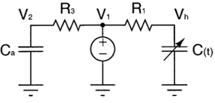
The pulsatile model shown in Figure 2-1 is a simplified version of the six-compartment hemodynamic model by Davis [4]. This simple model is made up of three segments: a venous, an arterial and a ventricular compartment. The time-varying compliance C(t) of the ventricle is represented by the time-varying capacitor, where C(t) is defined as the inverse of the piecewise linear elastance E(t):

1

C(t) = 1(2.1)

E(t)

The diodes D1 and D2 are assumed to be ideal and are in place to ensure

unidi-rectional current flow from the venous to the ventricular compartment, and then from the ventricular to the arterial compartment. The ohmic resistances R1, R2 and R3 represent the resistance to venous return, the aortic outflow resistance and the

arteriolar resistance, respectively.

The pulsatile model will be the basis for our analysis work, and we will derive an analytical solution to the model with a view to extending the results to a more elabo-rate circulatory model. The voltages V, V2 and Vh are of interest here, because they

represent the venous, arterial and ventricular pressures, respectively. During systole, the ventricular pressure exceeds the arterial pressure, causing the aortic valve to open and ventricular ejection to take place. For the pulsatile model, this corresponds to the period during which Vh is greater than V2, and D2 is forced into conduction as current

flows out of the time-varying capacitor C via R2 into the rest of the system. On the

other hand, V is much lower than Vh and D, is non-conducting, just like valves in the heart prevent back-flow of blood into the atria during the ejection phase.

R3

V1

R1

D1

Vh

D2

R2

V2

Ca

Figure 2-1: Simplified three-compartment circulatory model

As blood flows into the aorta, the arterial pressure rises along with ventricular pressure, and only a very small pressure difference exists between the ventricle and aorta, because the aortic valve opening offers little resistance to flow. This explains why the diodes are assumed to be ideal as we want the on-state potential difference to be as close to zero as possible. Systole is followed by a period of ventricular relaxation, or diastole, during which the aortic valve closes to prevent reverse flow and the bicuspid valve opens, allowing the ventricle to fill with blood from the atrium. In the pulsatile model, Vh _{is forced low by the rapidly decreasing elastance E(t) until}

D1 is forced into conduction, and current flows via R1 into C. D2 becomes

non-conducting as Vh drops below V2 during this phase.

2.2

Simulation in HSPICE

We implement the pulsatile model in HSPICE, a widely used device level circuit simulator, using the system parameters given in Table 2.1, where Vi0, V2 and Vho

denote the initial values of the voltage functions, respectively. The initial conditions are chosen as such in order to simulate realistic hemodynamic waveforms, in which the arterial pressure normally varies between a maximum (systolic) value of 120mmHg and a minimum (diastolic) value of 80mmHg. The initial conditions also ensure the system starts off in the end-diastolic state, which corresponds to that at the start of the piecewise linear elastance function.

Es

2.5 0.1 1 2 100 0.03 0.01 1 15.0337 91.2281 12.7383

Table 2.1: System parameters

The HSPICE code for the circuit simulation of the pulsatile model is shown here:

Pulsatile Heart Model * title

.option ingold=1 abstol=le-12 .option post=2

.option probe

.op

*set initial conditions

.ic V(n2)=15.0337 V(n4)=12.7383 V(n6)=91.2281

*define voltage source Vcap as piecewise linear elastance Vcap nc 0 PWL 0 0.1V, 0.3333 2.5V, 0.5 0.1V, 1 0.1V, R 0 Rgrd nc 0 1meg

*define circuit connection and component values Cv n2 0 C=100

R3 n2 n6 R=1

R1 n2 n3 R=0.03

Ch n4 0 C='1/V(nc)' CTYPE=1 *define time-varying capacitance using Vcap

R2 n5 n6 R=0.01 Ca n6 0 C=2

D1 n3 n4 diodel

D2 n4 n5 diodel

.model diodel D level=1 IS=1 *simulation of ideal diode

*transient analysis for t=10s at time step of 0.Ois

.tran O.Ois 10s

.print tran V(n2) V(n4) V(n6) V(nc) .end

The code consists of three main parts. The first part initializes the voltage func-tions using the initial condifunc-tions stated in Table 2.1. The second part "builds" the circuit model by defining the time-varying capacitance, the circuit connection be-tween the electrical components and the component values. The last part runs the simulation for 10s with a time-step of 10-2s, and generates the voltage waveforms as simulation output of the pulsatile model.

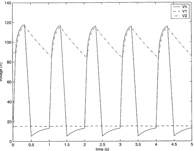
Figure 2-2 shows the voltage waveforms generated by the HSPICE simulation of the pulsatile model using the piecewise linear elastance. The period of the voltage waveforms is the same as the period T of the time-varying elastance E(t). The changes in Vh relative to V and V2 set the on-off states of the diodes, which in turn modify

the circuit and lead to further changes in the voltages. We will discuss the waveforms' characteristics in the next chapter when we study the waveforms in greater detail in order to derive an analytical solution to the pulsatile model.

140 120 100 C, 0) 80 60 40 20 A 0 0.5 1 1.5 2 2.5 3 3.5 4 4.5 5 time (s)

Figure 2-2: HSPICE simulation output of the pulsatile model using piecewise linear elastance -- Vh - - v1 -V2 \ \ / \/ ,j .1 I -

---- :i

~

-Chapter 3

Deriving the Analytical Solution

Deriving a closed-form analytical solution to the pulsatile model is made possible

by the piecewise linear elastance definition, which simplifies the numerical solution

of the governing differential equations. Due to the periodic nature of the elastance function, the steady-state voltage waveforms are periodic with the same period T. This simplifies the problem of deriving the analytical solution, as we only have to solve the problem over one cycle. The on-off switching of the diodes D, and D2, coupled

with the piecewise linear properties of the elastance function, segment each cycle period into seven distinct regions, which correspond to different elastance functions and diode states of the pulsatile model. As such, we will derive the analytical solution

by solving the governing differential equations for each region separately.

3.1

Dividing into Subproblems

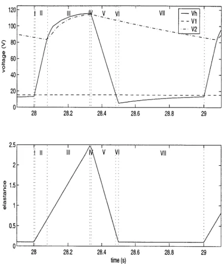
Figure 3-1 shows the steady-state voltage waveforms and the piecewise linear elastance function divided into seven regions over one cycle. The regions are demarcated such that each region is defined by a different linear elastance function, and a different circuit representation of the pulsatile model as determined by the on-off states of D1 and D2.

120 _{V VII Vh} --V1 100- -> 80- 60-0 40- 20-0 28 28.2 28.4 28.6 28.8 29 2.5 II II V VII 2-o1.5 0.5-0 28 28.2 28.4 28.6 28.8 29 time (s)

Figure 3-1: Steady-state voltage waveforms (top) and piecewise linear elastance func-tion (bottom) divided into seven regions over 1 cycle

Region

D,

D

E(t)

I on off linearly increasing

II off off linearly increasing

III off on linearly increasing IV off on linearly decreasing

V off off linearly decreasing

VI on off linearly decreasing

VII on off constant

Table 3.1: Definition of the 7 regions

3.1.1

Notation

To facilitate the mathematical derivation of the analytical solution, the following notation is adopted for the nth region:

start time tn ₁; venous voltage Vn(t)

end time tn; arterial voltage V2n(t)

time duration fn; ventricular voltage Vhn(t)

elastance En(t); charge on C Qhn(t)

The start time of Region I, which also corresponds to the start time of the cycle, is set to zero without any loss of generality. The time duration fn of the nth region

is defined to be the difference between the start and end times of the region, i.e., fn = tn - tn_1. VI(t) is assumed to be constant over one cycle, as it has a very small

peak-to-peak ripple of about O.4V. Therefore,

Vn(t) = V

(0)

n =

where V 1(0) is the initial condition of V(t) for the current cycle.

3.1.2

Approach Outline

We outline the general approach to deriving the analytical solution for the nth re-gion. First, the initial conditions are obtained directly from the end conditions of the preceding region within the same cycle. The equivalent circuit model and elastance function are defined for the region. The numerical solution of the first-order govern-ing differential equations is simplified through makgovern-ing reasonable assumptions and seeking polynomial approximations to complex integral functions, in order to derive closed-form expressions for Vn(t), V2n(t), Vh,(t) and Qhn(t). The time duration f,

is also computed to determine the end conditions for the region, which are used to initialize the succeeding region.

V2 R3 V A

R'

Ca

_-

_C(t)

Figure 3-2: Equivalent circuit model for Region I

3.1.3

Region I

Region I begins with the initial conditions V2 1(0) > V1I(O) > Vhl(O), and ends when

Vhl(t) rises to equal 11(t). Throughout this region, Vhl(t) is below both V11(t) and

V2 1 (t), which causes D1 to conduct and D2 to be non-conducting. The equivalent

circuit model for this region is shown in Figure 3-2, where D1 is replaced by a wire

and D2 by an open circuit. V11(t) is constant, and is represented by a DC voltage

source of magnitude V11(0). The potential difference V, across a capacitor is related

to its capacitance C and the stored charge

Q

Q

V=

- =QE

C

where we already established that the elastance E is the inverse of capacitance. In this region, the elastance is defined as a linearly increasing function:

El(t)

E

(3.3)

TS

The flow of current into the time-varying capacitor C increases the charge Qhl(t) stored on it. With E1(t) increasing linearly in this region, Vhl(t) increases according

to Equation 3.2. From Figure 3-1, we note that the time duration ti, which is defined as the time taken for Vhl(t) to equal V1 1(t), is very short at about 0.002s. As such, we assume the change in Qhi(t) to be small over this time interval, and Qhi(t) to be

constant: Vhl(O) Qhl(t)

E

E1(0)

Vhl(0)

(3.4)

V2 1(t) decreases exponentially with a time constant of CaR3, as current flows out of the capacitor Ca into the rest of the system. From the equivalent circuit model, we have a first-order governing differential equation in V2 1 (t):

Vn 1(t) - V2 1(t) CaV₂1(t) ₌ R3 I V 1(0) V2 1(t) - V2 1(t) +

(3.6)

The mathematical working in the numerical solution of the differential equation is omitted here (see Appendix A.1). By assuming a constant Qhl(t), we have derived closed-form voltage functions for Region I. The end conditions of the region is deter-mined by the time duration fl, which is the time taken for Vhl(t) to equal Vii(t):

V 1(fi) = Va(11)h

1 Vhl(O)(Es - Ed)

-V7u(O) EdT8 t+±V1(O)

EdTs

[V11(O) - Vhl(O)] EdTs

_(3.8)

Vhl(O)(Es - Ed)

By substituting f into Equation 3.3, 3.5 and 3.7, we have the initial conditions E2(0), Vh2(0), and 22(0), respectively, for Region II. Given that the region starts off

3.1.4

Region Il

V2

R3

V,

Vh

Ca

C(t)

Figure 3-3: Equivalent circuit model for Region II

Region II begins with Vh2(t) just higher than

V

to equal

V

(t).

causes both D1 and D2 to be non-conducting. The equivalent circuit model, when we

replace both diodes by open circuits, is shown in Figure 3-3. The initial conditions of Region II map directly to the end conditions of Region I:

E2(0) = E1

(fi)

Vh2(0) = Vhl(tl) (3.10)

V22(0) = V21(fl) (3.11)

Qh2(0) = Qhi(fil) (3.12)

In the equivalent circuit model, the time-varying capacitor C is disconnected from the main circuit by the non-conducting diodes, and no current flows in or out of it. The stored charge Qh2(t) therefore remains constant in this region:

Qh2(t) = Qh2(0) = Vhl(0)

(3.13)

Ed

The elastance function is the same as that for Region I, except for the initial condition

E₂(0):

E2(t) =

E

t +

Vh2(t) increases linearly with time according to Equation 3.2, since Qh2(t) is constant

and E2 (t) is linearly increasing.

_Vhl(0) [Es- Edt

Vh2(t) = E t + E2(0)

(3.15)

V2 2 (t) is always higher than V12 (t) but decreases exponentially with a time constant of CaR3, as current flows out of the capacitor Ca through the resistor R3 into the voltage

source. From the equivalent circuit model, we again have a first-order governing differential equation in 2 2(t): V12(t) - V22(t) CaV2 2(t) - (3.16) V22(t) V1 (t) 2 2(t) = - + (3.17) CaR3 CaR3 -> 22(t) = [V22(0) - VI(0)1 e- CaR3 + V,1(0) (3.18)

where the last equality follows from applying the result in Equation 3.7 directly. Now, we determine the end conditions for the region. The time duration t2, is defined as

the time taken for Vh2(t) to rise to V22(t):

Vh2(f2) = V22(f 2)

Vhl(0) Es - Ed 1 _ V

Ed TS 2 + E2(0) = [22(0) - Vj(0)] e CaR3 + V1(o) (3.19)

Given the structure of Equation 3.19, solving for t2 requires us to evoke the Lambert's

W function, which has the following mathematical definition:

w = lambertW(x) given that we' = x (3.20)

We implement Equation 3.19 in MATLAB and use the solve function to derive an expression for f2 in terms of the Lambert W's function:

1

2 E) [(V1(0)CaR3 lambertW(a) (E - Ed) - Vhj(0)E2(0)T + V1 (0)ETs]

V1((0)3(Es - E1)

where

1

a Vhl(O)CaR3(Es - Ed) [EdTs(V22(0) - V(0)1 e Vhl ()CaR3(Es-Ed)

(3.22)

The initial conditions E3 (0), Vh3(0) and V23(0) are obtained by substituting F2 into

Equation 3.14, 3.15 and 3.18, respectively. Lastly, the end time t2 is given by

t2 = f2+ tl (3.23)

3.1.5

Region III

Vh

R2

V2

R

Vi

(a)

Vh

=

V

R

V

0(t)a

(b)

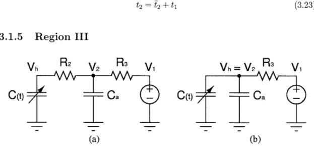
Figure 3-4: a) Equivalent circuit model for Region III b) Modified circuit model

(R

Region III corrresponds to the period of ventricular ejection, or systole, which begins when Vh₃(t) is just above V2 3(t), and ends when the elastance function E₃(t)

increases to the end-systolic value E,. Throughout the region, Vh3(t) is slightly higher than V23 (t), thereby forcing D2 into conduction while D1 remains non-conducting from

Region II. The equivalent circuit model is shown in Figure 3-4a. The initial conditions are determined from the end conditions for Region II:

E3(0) = E2(f2) Vh3(0) = Vh2(T2) V23(0) = V22(T2) Qh3(0) = Qh2(f2) (3.24) (3.25)

(3.26)

(3.27)

The elastance is defined as a linearly increasing function:

E3(t) =

E

At the start of the region, current flows from C to Ca as Vh3(0) is greater than V23(0).

However, Vh3 (t) continues to increase despite the outflow of charge from C, because E3(t) is increasing at a rate higher than that at which Qh3(t) is decreasing. V23(t)

increases and tracks Vh3(t) very closely, as current continues to flow into Ca. We assume R2 to be zero, as the potential difference between Vh and V2 is very small in

this reigon. However, this assumption does not allow for simulation of aortic stenosis. The modified circuit model for the region is shown in Figure 3-4b, and V23(t) is equal

to Vh3(t).

V23(t) = Vh3(t) (3.29)

Applying Kirchhoff's Current Law to the modified circuit model, we obtain a first-order governing differential equation in Qh3(t):

Qh3(t) + Vh3(t) R 13(t) + CaVh3(t) = 0 (3.30)

E3(t)Qh3(t) - V110)

QQ( + 3 + Ca[E3(t)QhU(t) + E(t)Qh3(t)] 0 (3-31)

E3(t) + R3CaE3(t) Vn1(0) R3[1 + CaE3(t)] R3[1 + CaE3(t)]

(3.32)

3t + y

t

Vj

d

Qh3(0)

where /3= -(E, - Ed) and -y CaE3(0)

+

solution is omitted here (see Appendix A.2). However, Qh3(t) is clearly not in closed-form, and we seek a polynomial approximation to the integral term in Equation 3.33

to simplify the solution. The end time of the region corresponds to the instant at which the elastance function equals Es.

(3.34)

(3.35)

The function

f(t)

[0, f3] using the system parameters from Table 2.1, and we see that the function is

well approximated by a constant c where

1 2 2 1.8 1.6 1.4 1.2 0.8- 0.6- 0.4-

0.2-{

(-

Figure 3-5: Plot of function

f(t)

40

function f(t) -constant c

t

Putting c into Equation 3.33, we have

1-1 ₁

Qh3(t)

(

)aeR3

and we have derived a solution for Qh3(t) in closed-form. Subsequently, we make use of Equation 3.37 to derive Vh3(t) and 23(t):

V2 3

(t)

= Qh3(t)E3(t)

(3.39)

3.1.6

Region IV

Region IV begins with both E(t) and Vh(t) at their peak values, and ends when Vh4(t) decreases to 24(t). However, from our assumption that R2 = 0 in Region III, we have

the initial conditions Vh4(0) = V24(0) which implies that the region ends as soon as it begins according to the definition of Region IV. As such, Region IV does not exist in our analytical solution! This is still a reasonable result since the time duration of the region is very short. For later discussion, we shall assume that Region V follows immediately after Region III.

3.1.7

Region V

Region V begins with Vh5(t) just below V25(t), and ends when Vh5(t) decreases to

V15(t). This region is similar to Region II in which both D1 and D2 are

non-conducting, and the equivalent circuit model shown in Figure 3-3 applies to Region V as well. The initial conditions of the region follow directly from the end conditions of Region III:

Vhs(0) = V25(0) = Vh₃

(t

)

As in Region II, Qh5(t) is constant, since the time-varying capacitor C is disconnected from the main circuit by the non-conducting diodes.

Qh((t) =

QV((0)

E

Es

However, the elastance is now defined as a linearly decreasing function:

E5 (t) Ed

t + Es

Tf

where T is the time taken for the elastance function to decrease linearly from E, to Ed. With Qh5(t) constant and E5(t) decreasing linearly, Vh5(t) decreases linearly

according to:

Vhs(t) = Qhs(t)ES(t)

Vh5(0)Ed

_{t + Es}

Es Tf

V25(t) is similar to V2 2(t) except for the initial conditions as the governing differential

equations are the same in both regions, and we apply the result from Region II directly:

V25(t) = [V25(0) - V11 (0)] e CaR3 + V(0) (3.45)

The time duration f5 is defined as the time taken for Vhs(t) to decrease to V1 5(t):

V15() = Vh5( N) (3.46) V1(0) = Vh5(0) Ed-Es

+ E

[F

(0)

3.1.8

Region VI

Region VI begins with Vh6(t) just below V 6(t), and ends when the elastance function

decreases to the diastolic value Ed. The end time of the region is therefore equal to the systolic time interval T, added to Tj:

t6= T, + Tf = 0.5T (3.50)

and

f6 = t6 - t5

(3.51)

V16 (t) is higher than Vh6 (t), which forces

D

off-state from Region V. Hence, the equivalent circuit model is the same as that in Region I (see Figure 3-2). The initial conditions correspond to the end conditions of Region V:

Vh6(0) Vh5 (f5) (3.52)

Qh6(0)

Qh

(4

)

(3.53)

V26(0) = V25(f5) (3.54) E6(0) E5 (f5) (3.55)

The elastance function is defined as a linearly decreasing function:

Ed- E

E6(t) =

E

E

Tf

Despite the flow of current into

C

R

,

is decreasing faster than the rate at which Qh6(t) is increasing. From the equivalent circuit model, we obtain a first-order governing differential equation in Qh6(t):

Qh₆(t) = V16(t) - Vh6(t)

(3.57)

RE

E6 (t) V 1(0)

Ed - Es

E(0)1

=- t +

Qh6(t)

V(

The mathematical working of the solution is omitted here (see Appendix A.3), and

we present the solution for Qh6(t) directly:

Es- Ed t2 _E6

[

_

Vh6(0)1

QhG(t) = e 2T

f Ri R1 Vi₁

(0)

It is not possible to obtain a closed-form expression for the integral term in Equation

3.60 as we are integrating a function of the form et2. We simplify the integral term by

Ed-ES t2+ E

seeking a polynomial approximation to the expression e 2Tf R1 R1 over the period

of interest. 1.1 1.08 1.06 .04 .02 0.01 1 0.005 0.015

Figure 3-6: Plot of function g(t) and the linear approximation h(t)

Ed-Es 2 E₆(O)

We define the function g(t) = e 2 Tf R1 R1 and plot g(t) over the interval [0,

46]

in Figure 3-6, using the system parameters from Table 2.1. The time period f 6 is very

44

- -e

- -function g(t)

-- linear approx. h(t)

short at about 0.015s, which allows us to approximate g(t) by a linear function h(t)

with marginal error.

Y-X

e

j

Y =

Substituting Equation 3.61 into Equation 3.60 and evaluating the integral term, we derived a closed-form solution for Qh6(t):

Es-Ed t2_ E6(O)t

Qh6(t) = e 2TfR1 R1 Vi(0) R,

Y - X

+

R1

xt)

Es]

Subsequently, we are able to derive a closed-form solution for Vh6(t):

Vh6(t) = Qh6(t)E(t) (3.64)

The governing differential equation in V26(t) is the same as that for V21(t), and we

apply the result from Region I directly to derive V26(t):

V

(t)

V

(0)]

(3.65)

3.1.9

Region VII

Region VII corresponds to the period during which the elastance function is constant at Ed, so

E7(t) = Ed (3.66)

The equivalent circuit model is the same as that in Region I and VI, as D1 and D2

remain in the on-state and off-state ,respectively. The initial conditions follow directly from the end conditions of Region VI:

Vh7(0) Qh7(0) = Vh₆( 6) = Qh6(f6) (3.67) (3.68) (3.62) (3.63)

V27(0) = V26() (3

From the equivalent circuit model, we have a first-order governing differential equation in Qh7(t), which is the same as that in Region VI:

__ V17(t) - Vh7(t) Qh7(t)=

R,

E

R

Qh

e

V1(0)

R

V

(0)

R1

+() V1 (0)

The mathematical working of the solution is shown in Appendix A.4. Here, we again make use of the results from Region I to derive V₂₇(t):

V

(t) = [V

(0)

V1(0)]

The end of the region corresponds to the end of the cycle , and so

t7 = T (3.75)

(3.76)

f7 = t7 - t6

3.1.10

Initializing the Next Cycle

We have so far successfully derived closed-form expressions for the voltage functions

Vi(t), V2(t) and Vh(t) for all seven regions within one cycle, by solving first-order

differential equations and making reasonable assumptions to simplify complex integral

46

(3.70)

(3.71) (3.69)

functions. A method of setting up the new initial conditions for the next cycle is required to implement the beat-to-beat propagation of the analytical solution. We denote the new initial conditions by Vnew(0), V21new(0) and Vhlnew(0), respectively.

V21new(0) and Vhnew(0) are obtained directly from the end conditions of Region VII

from the preceding cycle:

V2 new(0) = V27(7) (3.77)

Vhnew(0) Vh7(f7)

(3.78)

An expression for Vinew(0) is obtained by applying the principle of charge conserva-tion, which requires the total charge in the system at the start of the new cycle to be

equal to that at the start of the last cycle:

CvViinew(0) + CaV21new(O) + Vhlnew (0) = CvV11

(0)

(3.79)

Ed E

Vn1(0|CV + Vh1 (0) + V21(0)Ca - Vhlnw(O) - V21new(0)Ca

> V1new(0) = Ed Ca Ed (3.80)

Cv

In summary, we have derived a closed-form analytical solution to the pulsatile model, which computes V(t), V2(t) and Vh(t) recursively over many cycles given a set of

pre-defined initial conditions. Starting from Region I, we apply the initial conditions to the voltage functions corresponding to Region I, which then compute V1(t), V2(t)

and Vh(t) until the end of the region, after which the voltage functions corresponding to Region II take over. This carries on until we reach the end of Region VII, which also marks the end of the cycle. At this point, we use Equation 3.77, 3.78 and 3.80 to determine the new initial conditions to Region I of the following cycle, and the process repeats.