Approximation algorithms for rapid evaluation and optimization of architectural and civil structures

Approximation Algorithms for Rapid Evaluation and

Optimization of Architectural and Civil Structures

by

Stavros Tseranidis

BS, MS in Civil Engineering, Department of Civil Engineering - Polytechnic School

Aristotle University of Thessaloniki, 2014

Submitted to the School of Engineering

in Partial Fulfillment of the Requirements for the Degree of

ARCHNE

MASSACHUSTTIS INSTIITUTE OF TECHNO-LOGY

OCT 21 2015

LIBRARIES

Master of Science in Computation for Design and Optimization

Massachusetts Institute of Technology

@ 2015 Stavros Tseranidis. All rights reserved.

The author hereby grants to MIT permission to reproduce and to distribute publicly paper and electronic copies of this thesis document in the whole or in part in any medium now known or hereafter created.

Signature of Author:

S ignature redacted...

School of Engineering August 7, 2015

Certified by:

Signature redacted

Caitlin T. Mueller Assistant Professor, Building Technology Thesis Supervisor

Signature redacted

A c c e p te d b y : -... ..- -...

Nicolas G. Hadjiconstantinou Professor, Mechanical Engineering Co-Director, mputation for Design and Optimization (CDO)

Approximation Algorithms for Rapid Evaluation and

Optimization of Architectural and Civil Structures

by

Stavros Tseranidis

Submitted to the School of Engineering

on August 7, 2015 in Partial Fulfillment of the Requirements

for the Degree of Master of Science in Computation for Design and Optimization

Abstract

This thesis explores the use of approximation algorithms, sometimes called surrogate modelling,

in the early-stage design of structures. The use of approximation models to evaluate design

performance scores rapidly could lead to a more in-depth exploration of a design space and its

trade-offs and also aid in reducing the computation time of optimization algorithms. Six

machine-learning-based approximation models have been examined, chosen so that they span a wide

range of different characteristics. A complete framework from the parametrization of a design

space and sampling, to the construction of the approximation models and their assessment and

comparison has been developed. New methodologies and metrics to evaluate model

performance and understand their prediction error are introduced. The concepts examined are

extensively applied to case studies of multi-objective design problems of architectural and civil

structures. The contribution of this research lies in the cohesive and broad framework for

approximation via surrogate modelling with new novel metrics and approaches that can assist

designers in the conception of more efficient, functional as well as diverse structures.

Key words: surrogate modelling, conceptual design, structural design, structural optimization

Thesis supervisor: Caitlin T. Mueller

Acknowledgements

First and foremost, I would like to sincerely thank my advisor, Professor Caitlin Mueller, for giving

me such an interesting topic and guiding me throughout this research. The knowledge I acquired

from her through our meetings, discussions and her courses at MIT are extremely valuable to me.

She provided me with new insights and perspectives on structural engineering, design,

computational approaches and algorithms. Her course titled "Computation for Structural Design

and Optimization" has been one of my most meaningful and thought-provoking experiences at

MIT. For all that I am truly grateful.

I would like to thank Professor Jerome Connor and Doctor Pierre Ghisbain who gave me the

opportunity to be a Teaching Assistant in their courses and trusted me with such an important

task. Collaborating with them has been a great honor for me.

I would also like to thank Professor John Ochsendorf for welcoming me to his group and exposing

me to new fields in structural engineering and beyond.

Finally, I would like to thank all the students in the Digital Structures Group and the Structural

Design Lab. Especially, Nathan Brown for providing me with his datasets, which were crucial for

my research.

Table of Contents

1. Introduction ... 15

1.1 Structural optim ization ... 15

1.2 Need for com putational speed ... 16

1.3 Surrogate m odelling...17

1.4 Research question...18

1.5 Organization of thesis ... 18

2. Background ... 19

2.1 Surrogate m odelling on structural designs ... 19

2.2 M odel types ... 21

2.3 Error in surrogate m odels ... 22

2.4 Robustness in surrogate m odelling... 24

2.5 Unm et needs, open questions ... 25

3. M ethodological fram ework ... 27

3.1 Surrogate m odelling procedure ... 27

3.2 M odel types ... 28

3.2.1 Neural Networks (NN)... 28

3.2.2 Random Forests (RF) ... 30

3.2.3 Radial Basis Function Networks (RBFN) ... 31

3.2.4 Radial Basis Function Networks Exact (RBFNE)... 32

3.2.5 M ultivariate Adaptive Regression Splines (M ARS) ... 33

3.2.6 Kriging regression (KRIG)... 34

3.3 Norm alization... 36

3.4 Sam pling... 37

3.4.1 Grasshopper sam pling ... 37

3.5 Design exam ple...39

3.6 Rem oving outliers ... 42

3.7 Sum m ary ... 45

4. Visualization and error...47

4.1 Understanding error ... 47

4.4 Rank error m easures...56

5. Robust model com parison ... 61

5. Sing le run... 61

5.2 M ultiple runs ...Gr ..t... 62

5.3 Summary ... 65

6. C ase stu d ie s ... 67

6.1 Case study 1 - Grid truss ... 67

6.1.1 Building ..-A... tte.. na... ... 67

6 .1 .2 B rid ge .. ... 7 1 6.2 Case study 2 - P r tru su r de ... ... ... ... 74

6.3 Case study 3 - Airport term inal ... 76

7. Results .... rp rtr... m ... 81

7.1 Case Study 1 - Grid Truss Bridge ... 81

7.2 Case Study 2 - P Structure... 84

7.3 Case Study 3 - Airport terminal ... ... ... 91

7.4 Summary table .t... 102

8. Conclusions... 105

8.1 Summary of contributions ... 105

8.2 Potential im pact... 105

8.3 Future work dxA A r ...n.. |E e... 106

8.4 Concluding remarks...107

References ... ... 109

Appendix A: Airport terminal

I

I

NN - Neural Networks ... ... 113

RF - Random Forests ... 116

RBFN - Radial Basis Function Networks x... ... ... 118

RBFNE - Radial Basis Function Networks Exact ... 120

M ARS - M ultivariate Adaptive Regression Splines...123

KRIG - Kriging Regression... 126

Appendix B: Case study scatter plots ... ... 129

Energy Overall __ Boston __ PI Structure ... 129

Heating+Cooling+Lighting - Boston __ PI Structure ... 130

Heating _ Boston __ PI Structure ... ... 133

Lighting _ Boston __ PI Structure... ... 134

Energy Overall _ Sydney _ PI Structure...135

Heating+Cooling+Lighting _ Sydney __ PI Structure ... 136

Structure _ Sydney _ PI Structure ... 137

Cooling _ Sydney - PI Structure ... ... 138

Heating _ Sydney - PI Structure... .... 139

Lighting _ Sydney _ PI Structure ... 140

Energy Overall - Abu Dhabi - Airport terminal ... 141

Cooling+Lighting _ Abu Dhabi - Airport terminal ... 142

Structure _ Abu Dhabi __ Airport terminal...143

Cooling _ Abu Dhabi _ Airport terminal...144

Lighting _ Abu Dhabi _ Airport terminal ... 145

Energy Overall - Abu Dhabi Rotated _ Airport terminal...146

Heating+Cooling+Lighting __ Abu Dhabi Rotated _ Airport terminal ... 147

Structure __ Abu Dhabi Rotated __ Airport terminal ... 148

Cooling _ Abu Dhabi Rotated - Airport terminal ... 149

Lighting _ Abu Dhabi Rotated - Airport terminal ... 150

Energy Overall __ Boston _ Airport terminal...151

Heating+Cooling+Lighting __ Boston _ Airport terminal ... 152

Structure _ Boston __ Airport terminal ... 153

Cooling _ Boston _ Airport terminal ... 154

Heating _ Boston _ Airport terminal...155

Lighting _ Boston _ Airport terminal...156

Energy Overall __ Boston Rotated __ Airport terminal ... 157

Heating+Cooling+Lighting _ Boston Rotated __ Airport terminal ... 158

Structure __ Boston Rotated - Airport terminal ... 159

Cooling _ Boston Rotated - Airport terminal ... 160

Heating _ Boston Rotated - Airport terminal ... 161

Lighting _ Boston Rotated _ Airport terminal...162

Energy Overall _ Sydney - Airport terminal...163

Heating+Cooling+Lighting _ Sydney _ Airport terminal...164

Cooling _ Sydney _ Airport terminal ... 166

Heating _ Sydney _ Airport terminal ... 167

Lighting _ Sydney _ Airport terminal ... 168

Energy Overall _ Sydney Rotated _ Airport terminal ... 169

Heating+Cooling+Lighting _ Sydney Rotated - Airport terminal ... 170

Structure _ Sydney Rotated __ Airport terminal ... 171

Cooling _ Sydney Rotated - Airport terminal ... 172

Heating _ Sydney Rotated _ Airport terminal... 173

List of Mathematical Symbols

SYMBOL MEANING

X Matrix nXp containing the input variables' values

y Vector of dimension n containing the original, actual output values

h Vector of dimension n containing the predicted output values

yi Actual output value i

hi Predicted output value i

n Number of samples; design observations

Abbreviations

NN - Neural Networks RF - Random Forests

RBFN - Radial Basis Function Networks

RBFNE - Radial Basis Function Networks Exact

MARS - Multivariate Adaptive Regression Splines

MSE - Mean Squared Error RMSE - Root Mean Squared Error MRE - Mean Rank Error

TMRE

TRE - Top Ratio Error TFE - Top Factor Error REM - Rank Error Measures AAE - Average Absolute Error

MAE

Maximum Absolute Error

RAAE - Relative Average Absolute Error

RMAE

Relative Maximum Absolute Error

1. Introduction

The engineering design process is a demanding endeavor. It is a mix of analytical tools with human intuition. The design of new structures lies on the same category. It is complex; it involves multiple objectives and numerous parameters. The work on this thesis contributes in this area and has the goal to empower designers to achieve more efficient structures, by using a type of approximation technique called surrogate modelling.

1.1 Structural optimization

To the extent of the feasible and the realistic, optimization is strived for in engineering design. In structural engineering, specifically, optimization is a process that involves many physical constraints, such as construction, material production and transportation, cost, safety and many more. At the same time, in the discipline of architecture, more abstract considerations are prioritized in design; functionality, aesthetics and human psychology just to name a few. Both disciplines are combined in practice, sharing the same goals to produce a single result.

Unlike other engineering disciplines, the optimization objective goals and constraints are not always easily quantified and expressed in equations, but rather require human intuition and initiative to materialize. For this reason, structural optimization has yet to reach its full potential. With modern computers and tools available, this potential is beginning to be realized. There are a few examples where it has been successfully applied to buildings, such as in projects by Skidmore Owings & Merrill (SOM) [1], shown in Figure 1. To illustrate the breadth of designs for braced frame systems, another one by Neil M. Denari Architects is shown in Figure 2 (High Line 23, New York City [2]). While this design is not structurally optimized, its architectural success is closely linked to its structural system and geometry. So, in the structural design optimization, there needs to be a balance between quantitative and qualitative objectives. P!2 P p--P P Pt2 P p P P 461

Figure 2:

Braced frame system, Denari Architects (Image from [2])

On the one hand is the quantitative aspect of optimization. Structural evaluation simulations as well as energy simulations, which compute the energy consumed by a building, often require significant computational power, increasing with the complexity and size of the project. Thus, optimization algorithms can usually require substantial execution time. To put this in context, for energy simulations included in the case studies, the time required for one sample evaluation was approximately 25 sec, which impedes a free-flowing design process. This fact slows down the design process. On the other hand, because of the qualitative nature of this type of design with the hard-to-quantify considerations as described above, many iterations are required and the result is never likely to come up from a single optimization run. In practice, the combination of slow simulation and problem formulation challenges means that optimization is rarely used in the design of architectural and civil structures. In fact, even quantitatively comparing several design alternatives can be too time-consuming, resulting in poor exploration of the design space and likely a poorly performing design.

1.2 Need for computational speed

The exploration of the design problem and various optimal solutions should ideally happen in real time, so that the designer is more productive. Research has shown that rapid response time can result in significant productivity and economic gains [3]. "Improved individual productivity is perhaps the most significant benefit to be obtained from rapid response time" [3]. The upper threshold for computer response time for optimal productivity has been estimated at 400ms and is commonly referred to as the Doherty threshold [3]. This threshold was originally developed in the 1980s for system response of routine tasks, like typing. Today, however, software users expect similarly rapid response for any interactions with

response from the computer can benefit not just rote productivity, but also creative thinking. The concept

of flow is used in psychology to describe "completely focused motivation"; when a person gets fully immersed and productive. It was thoroughly studied by M. Csikszentmihalyi [4] and among the components for someone to experience flow, "immediate feedback" is listed.

The first way to implement the "immediate feedback" effect in computer response is by increasing the available computational power. This can be achieved by either increasing the processing power of a computer or by harnessing parallel and distributed computing capabilities. The other way is to use different or improved algorithms. This thesis focuses on the second approach, investigating algorithms that improve computational speed for design-oriented simulation through approximation.

1.3 Surrogate modelling

Among possible approximation algorithms, this thesis considers surrogate modelling algorithms, a class of machine learning algorithms, and their use in making computation faster and allowing for more productive exploration and optimization in the design of buildings.

Machine learning is about creating models about the physical world based only on available data. The data are either gathered though physical experiments and processes, or by computer-generated samples. Those samples are then fit to an approximation mathematical model, which can then be used directly as the generating means of new representative data samples. In surrogate modelling specifically, the data is collected from simulations run on the computer.

Similar techniques are being used successfully in many other engineering disciplines, but have not been studied and applied extensively to the architectural and structural engineering fields. This research investigates these techniques and evaluates them on various related case studies. Focus is given in the development of a holistic framework that is generalizable.

f

12

x

Figure 3: "Many surrogates may be consistent with the data" (Figure from [5])

Figure 3 displays a core concept in surrogate modelling. The circles represent the available data, with many different models being able to fit them. The art in surrogate modelling is to choose the one that will also fit new data well.

1.4 Research question

This thesis considers two key questions:

Is surrogate modelling a viable methodology to use in this field?

The main focus of this thesis is to examine the use of surrogate modelling in the design of architectural and civil structures as a method to rapidly explore the design space and obtain more efficient solutions.

It applies it in case study problems and tests its applicability and effectiveness.

How robust is surrogate modelling?

Questions of how good an approximation method is are addressed. Also considered are matters of how accurate a model is and how its error value and variability can be estimated. Methods for this purpose are proposed and applied.

1.5 Organization of thesis

First, a literature review of the existing research in surrogate modelling, its application in structural engineering problems, model types and error assessment methods is outlined in Chapter 2. Chapter 3 is an overview of the main features of the methodology framework used, including assumptions and descriptions of the models used. Sampling and outlier removal techniques are also discussed. Chapter 4 is dedicated to explaining the error assessment and visualization methods used throughout the rest of the thesis. Chapter 5 introduces the proposed method for robust model comparison, whose use is then illustrated through the case studies in Chapters 6 and 7. Specifically, Chapter 6 introduces the case study problems, the parameters examined and the analysis assumptions, while Chapter 7 presents all the numerical results obtained for comparing model performances and assessing them individually for all the case study problems. The original contributions, findings and future considerations are summarized in Chapter 8. Finally, in the Appendix, a sample of the outputs of the developed MATLAB framework is presented for one case study (Airport terminal) and for one performance score approximation (Energy Overall).

2. Background

To avoid a computationally expensive simulation, one approach is to construct a physical model that is simpler and includes more assumptions than the original. This process is very difficult to automate and generalize and requires a high level of expertise and experience in the respective field. A more general approach is to substitute the analytical simulation with an approximate model (surrogate) that is constructed based purely on data. This approach is referred to as data-driven or black-box simulation. The reason is that the constructed approximation model is invariant to the inner details of the actual simulation and analysis. The model has only "seen" data samples that have resulted from an "unknown" process, thus the name black-box. This thesis addresses data-driven surrogate modelling.

The two main areas in which surrogate modelling can be applied are for optimization and design space exploration. Specifically, an approximation (surrogate) model can be constructed as the main evaluation function for an optimization routine or just in order to explore a certain design space in its entirety, better understand variable trade-offs and performance sensitivity. For optimization, it is often used when there are more than one optimization objectives, thus called multi-objective optimization (MOO), and the computational cost of computing them is significant.

2.1 Surrogate modelling on structural designs

Several years ago, when the computational power was significantly less than that of today, one available today, scientists started to explore the possibility of adapting approximation model techniques in intensive engineering problems. One of the first attempts of this kind in the field of structural engineering

by Schmit and Miura [6] in a NASA report in 1976. A review of the application of approximation methods

in structural engineering was published by Barthelemy and Haftka in 1993 [7]. The methods explored in this review paper are response surface methodology (RSM) as well as neural networks (NN). It was mentioned that more methods will emerge and the practice is going to expand. In fact, today, although the computational power has increased exponentially from twenty years ago, the engineering problems that designers face have also increased dramatically in scale and therefore surrogate modelling has been studied and applied extensively.

Hajela and Berke wrote a paper in 1992 [8] solely dedicated to an overview of the use of neural networks in structural engineering problems. They mentioned that this approximation technique could be useful in the more rapid evaluation of simulations such as non-linear structural analysis. Neural networks and approximation models have still great potential in this field today, when non-linear structural analysis is very frequently performed. Researchers have been using approximation algorithms in the structural engineering field for various problems such as for the dynamic properties and response evaluation and optimization of structures [9], for seismic risk assessment [10] and for energy MOO simulations [11]. Energy simulations are extensively examined in this thesis, since they are usually extremely expensive computationally, and at the same time their use and importance in building and infrastructure design is increasing today.

The use of approximation algorithms in conceptual architectural/structural design was very interestingly examined by Swift and Batill in 1991 [12]. Specifically, for truss problems, with the variables being the positions of some nodes of the truss and the objective the structural weight, a design space was sampled and later approximated using neural networks. A representative figure from this paper can be seen in Figure 4, where the initial base structure and the variable ranges are shown in Figure 4a, while the best designed obtained from the neural network approximation is on Figure 4b.

(a) Resian C 7 1 X st 13 In 7 1 Y .5 13 In 10 in: tk C 5k

T-

6k

Figure 4:

Ten-bar truss (a) design space and (b) best design resulting from NN model (Image from

[12])

A similar approach was followed by Mueller [13], with a seven-bar truss problem examined being shown in Figure 6a. The variables were again the positions of the nodes and specifically the vertical nodal positions as shown along with their ranges in Figure 6a. The design space (with the structural weight as the objective score) computed analytically, without approximation is shown in Figure 6b. The approximated design space for different models is shown in Figure 6. Details on the approximation models used later are presented in the following section on model types.

50 20 -30 . -50 *2

1.8

I

-80

Figure 5:

Seven-bar truss (a) variables and (b) analytically computed design space (Image from

2 181.8 1.8 1.6 1.6 1.6 1.4 1.4 1.4 1.2 1.2 1.2 0.8 0.8 0.8

Figure 6:

Seven-bar truss approximated design space for different parameters (Image from [13])

It is also worth mentioning that surrogate modelling is being used extensively in the aerospace industry. The basic principles remain the same across disciplines since the methodology relies solely on data. Queipo et al. [5] have made a thorough overview of the common practices of surrogate modelling. They also applied those techniques in an MOO problem from the aerospace industry. Another comprehensive survey of black-box approximation method for use in high-dimensional design problems is included in [14].

There exist attempts of integrating performance evaluation into parametric design in architectural and civil structures. Mueller and Ochsendorf [15] considered an evolutionary design space exploration, Shi and Wang [16] examined performance-driven design from an architect's perspective, while Granadeiro et al. [17] studied the integration of energy simulations into early-stage building design. All of those interesting approaches could benefit by the use of surrogate modelling, which is the main contribution of this thesis.

2.2 Model types

Several methods have been developed over the years to approximate data and have been used in surrogate modelling applications. Very common ones include polynomial regression (PRG) and response surface methodology (RSM) [18], in which a polynomial function is fitted to a dataset using least squares regression. This method has been used in many engineering problems [5].

One of the most widely used surrogate modelling method in engineering problems is Kriging (KRIG). Since it was formally established in the form it is used today [19], it has been applied extensively ([10], [5], [20]). Gano et al. [21] compared Kriging with 2" order polynomial regression. Chung and Alonso [20] also

compared 2nd order RSM and Kriging for an aerospace case study and concluded that both models

performed well and are pose indeed a realistic methodology for engineering design.

Another very popular model type are artificial neural networks (referred as NN in this thesis). Extensive research has been performed on this type of model ( [5], [8] ). Neural networks are greatly customizable and their parameters and architecture are very problem specific.

A special type of neural network is called radial basis function network (RBFN) and was introduced by Broomhead and Lowe [22] in 1988. In this network, the activation function of each neuron is replaced by

a gaussian bell curve function. A special type of RBFN imposes the Gaussian radial basis function weights such that the networks fits the given data with zero error. This is referred to as radial basis function network exact (RBFNE) and its main drawback is the high possibility that the network will not generalize well on new data. Those two types of models, RBFN and RBFNE, are explained in more detail in Chapter 3 as they are studied more extensively in this thesis.

Radial basis functions can also be used to fit high dimensional surfaces from given data. This model type is called RBF [23] and is different from the RBFN model. RBF models can also be referred to as gaussian radial basis function models [5]. Kriging is similar to RBF, but it allows more flexibility in the parameters. Multivariate adaptive regression splines (MARS) is another type of model. This performs a piecewise linear or cubic multidimensional fit to a certain dataset [24]. It can be more flexible and capture more complex datasets, but requires more time to construct.

Jin et al. [25] performed a model comparison for polynomial regression, Kriging, MARS and RBF models. They used 13 mathematical problems and 1 engineering one to perform the comparisons. Many other references for papers that performed comparisons between those and other models are also included in

[25]. An important feature outlined in this paper was that it set five major aspects to compare the models.

Those were accuracy, robustness (ability to make predictions for problems of different sizes and type), efficiency (computational time to construct model), transparency (ability of the model to provide information about variable contribution and interaction) and conceptual simplicity. Those issues are examined in following sections in the present thesis.

Finally, the existing MATLAB-based framework SUMO [26], implements support vector machines (SVM)

[27] (a model type frequently used for classification), Kriging and neural network models, along with the

sampling and has been used in many applications such as RF circuit modelling and aerodynamic modelling

[26].

A framework with NN, Random Forests (RF) which have not extensively been applied in structural

engineering problems, RBFN, RBFNE, MARS and KRIG models was developed and tested in case study problems in the current thesis to extend the existing research and available methodologies for structural design.

There is a lack of extensive model comparison and their application on problems for structural engineering and building design specifically; this thesis addresses this need to move beyond existing work.

2.3 Error in surrogate models

The most important error required to assess an approximation model is what is called its generalization error. This is more thoroughly examined in the following section about robustness. In the current section, ways to quantify a model's performance on a given set of data are discussed. When the actual performance calculated from the analytic simulation is known for a set of data, and the respective performance from an approximation model is calculated, then the error of the predicted versus the actual

One of the most common ones is R2

, which refers to the correlation coefficient of the actual with the

predicted values. A value closer to 1 indicates better fit. This is extensively discussed in this thesis in Chapter 4 about error. Other common measures are the Mean Squared Error (MSE) and its root, the Root Mean Squared Error (RMSE). The Average Absolute Error (AAE) and the Maximum Absolute Error (MAE) are other options, along with Relative Average Absolute Error (RAAE) and the Relative Maximum Absolute Error (RMAE). MAE is generally not correlated with R2 or AAE and it can indicate whether the model does not perform well only in a certain region. The same holds true for RMAE, which is not necessarily correlated with R2

or RAAE. However, R2

, RAAE and MSE are usually highly correlated [25], which makes

the use of more than one of them somewhat redundant. Gano et al. [21] used R2

, AAE and MAE for the

model comparisons they studied, while .in et al. [25] used R2

, RAAE and RMAE.

The above mentioned error metrics are summarized along with their formulas on Table 1.

Error metric Formula

1 MSE - I 2 n 2 RMSE 1- 2 n )Ij - h₁)2 3 R 1 - fL( Z'1(y, - y)2 4 AAE X1 1 Ivj -n 5 RAAE =1Iy1-hiI n -STD(y)

6 MAE max(|y1 - h,1,|y2 - h21, --- Iyt - hi1) max(Iyj - h, 1,y2 - h2 1, 1y - hi1)

STD(y)

Table 1: Common surrogate modelling error metrics (y: actual, h: predicted value)

Error measures which provide a more direct and comprehensive quantitative model performance metric are lacking, and some alternative approaches to address this are presented in this thesis. Error measures based on a model's performance on the rank of the samples [13] are also studied. Special focus is also given to the visualization of the results and it is argued that normalization and visualization can have a significant impact in understanding error and are problem specific.

2.4 Robustness in surrogate modelling

As mentioned in the beginning of the previous section, it is crucial for a surrogate modelling application to have an acceptable generalization error. This refers to an error estimate of the model on new data. In this context, new data means data samples that have not been used at any point in the construction of the model. One can realize that this is indeed the most important error required since the rapid generation of accurate new data performance is the main objective of the construction of the surrogate model in the first place.

To estimate the generalization error, several techniques exist. Those are explained in detail in Queipo et al. [5] and Viana et al. [28]. The simplest one is to split a given dataset into train and test data, construct the model with the train data and then compute the error in the test data and take this as an estimate of the generalization error. Another technique is called cross-validation (CV), in which the original dataset is split into k parts and the model is trained with all the parts except one, which is used as the test set of the previous case. The procedure is then repeated until each one of the k sets has served as the test set. By taking the mean of the test set errors, a more robust generalization error estimate is produced. Another advantage is that a measure of this error's variability can be obtained by taking, for example, the standard deviation of the computed k test set errors. If this procedure is repeated the same number of times as the number of samples in the original dataset, which means that only a single sample is used every time as the test set, then this measure is called PRESS and the method leave-one-out cross validation [281. The last method to obtain a robust generalization error measurement is through Bootstrapping. According to the known definition of the bootstrap (sample with replacement), a certain number of bootstrap samples (datasets) are created as training and test sets. Then the error estimate and its variability calculation procedure is similar to the CV method. For the Bootstrapping method to produce accurate results, a large number of subsamples is usually needed [28].

This thesis attempts a combination of the aforementioned techniques frequently used in the surrogate modelling context with the common practice of machine learning applications (train/validation/test set partition) to obtain a measure of robustness as well as accuracy.

Another way to interpret robustness is to consider it as the capability of the approximation model to provide accurate fits for different problems. This again can be measured by the variance of accuracy and error metrics. However, the scope of this thesis is to examine the deployment of approximation models for case study design problems and not to comment on a model's more general predictive ability regarding

its mathematical properties.

Finally, to increase robustness, one could use ensembles of surrogate models in prediction [5]. This means that several models are trained and their results are averaged with a certain scheme to obtain a prediction. Models of this type are Random Forests (RF), which are studied in this thesis and explained in more detail in the next chapter.

2.5 Unmet needs, open questions

As described in the previous sections, the field of surrogate modelling in engineering design is very rich. However, its use in the design of architectural and civil structures is limited compared to other engineering disciplines. There is a need for a comprehensive study of its use in this area to examine whether they can be feasible and realistic in practice. The thread of their use in conceptual structural design was left in 1992 [12] and picked up recently [13]. An extension of the study in this field is necessary, since the advantages that rapid exploration and optimization can have in early stage structural design could be significant. While many model types have been investigated, few have been applied to real problems in this field. There is also a field within a field in error estimation and visualization of approximation models, which needs to further be explored. Specifically, what other types of error metrics and visualization techniques can be used in surrogate modelling applications are among the questions this thesis will address. A main concept that is addressed and pointed out throughout the thesis is that the prediction results of a model should be visualized instead of just obtaining an error metric value.

Model robustness considerations are also examined thoroughly, proposing a methodology that is focused on approximating data by combining ideas from various surrogate modelling/machine learning contexts and has the goal of broad applicability and scalability in architectural and civil structure design applications.

--0

0

+

$.;

aC

3. Methodological framework

This chapter outlines in detail the basic components used throughout this research, the proposed methodology and the case studies, all thoroughly explained in the following chapters. In general, the framework developed is based on sampling a design scape in the first place and then constructing and assessing the surrogate models. For the sampling part, the Rhino software and the Grasshopper plugin were used. They are parametric design tools very broadly used in architectural design. As for the surrogate modelling part, the framework and all of the analysis was performed in MATLAB. References to the specific functions and special capabilities of the software are placed in context in the text.

3.1

Surrogate modelling procedure

The basic surrogate modelling procedure consists of three phases; training, validation and testing. A separate set of data is needed for each of those phases. During the training phase, a model is fit into a specific set of data, the training set. The fitting process refers to the construction of the mathematical model; the determination of various weighting factors and coefficients. In the next phase, the trained model is used on a different set of data, the validation set, and its prediction error on this set is computed. The first two steps of training and validation are repeated several times with different model parameters. The model that produced the minimum error on the validation set, is then chosen for the final phase of testing. During testing, another dataset, the test set, is used to assess the performance of the model chosen from the first two steps (minimum validation set error).

The steps are shown schematically in Figure 7. Each model type can have multiple parameters which define it. Those are referred to as nuisance parameters, or simply parameters in the following chapters. Different nuisance parameters can result in different levels of model fit and accuracy. Choosing the best nuisance parameters for a given model type is the goal of the validation phase as described in the previous paragraph. The test phase is for verification of the model's performance on a new set of data, never previously used in the process (training or validation). More details can be found in [27].

Train

Val.

Test

Model

3.2 Model types

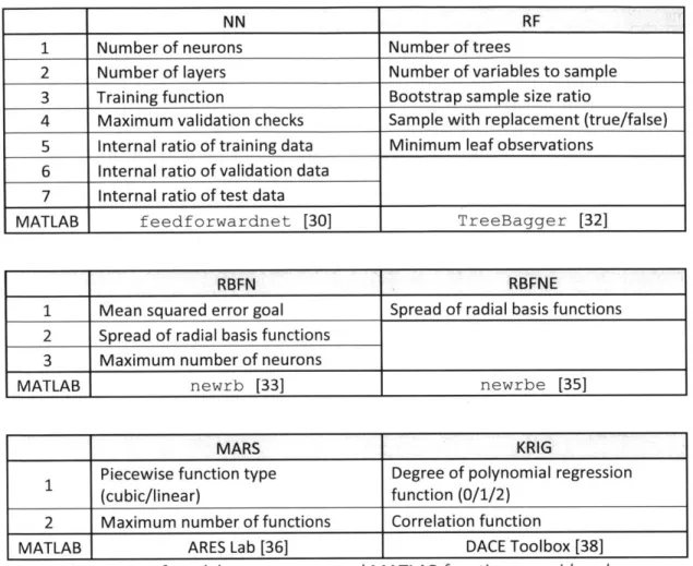
The utilization of approximation models, referred to as surrogate models or machine learning algorithms in different disciplines, aims at prediction. A model is essentially a procedure that acts on input data and outputs a prediction of a physical quantity. Previously computed or measured values of the physical quantity at hand, along with the corresponding input variables, are used to create/train the model, which can afterwards be used to make rapid predictions on new data. There are numerous different surrogate modelling algorithms and architectures. In the following section, the models examined in the present thesis are introduced. Lists of the parameters affecting each model which were considered are also included. All the model parameters considered and MATLAB functions used are summarized in Table 10.

3.2.1 Neural Networks (NN)

The human brain consists of billions of neurons connected together. Signals of different intensities are transmitted throughout this network. All the input signals to a neuron are summed together and if the sum exceeds a threshold value, then the specific neuron is triggered. The neural network architecture observed in biological procedures has been studied and has been adapted as a mathematical construct, forming what are known as Artificial Neural Networks. This computational model was firstly proposed in 1943 [29] and has been refined over the years.

The typical single-layer neural network architecture is shown in Figure 8. Multiple hidden layers can be inserted in the architecture.

Output layer

-.... _{Hidden layer}

Input layer

Figure 8: Single-layer neural network architecture (Image from [27])

The procedure to obtain a prediction from a single-layer neural network is the following:

The input vector X is multiplied by the respective weights of the hidden layer connections and the sum is obtained for each neuron. Then at each neuron, this sum is passed through an "activation" function. The procedure is repeated again for the output layer and the results from each output neuron is the prediction vector. Equation 1 describes the calculation procedure in a single neuron.

Zm=-(aom + a'nX), m = 1, ... , M

Equation 1: Single neuron calculation [27]

For each neuron the input vector X is multiplied by the respective weights of each connection

and the results are summed (with the addition of a constant "bias" term aom). This sum is then

passed through an "activation function" a(x), which for the results of the present thesis was

chosen to be the tan-sigmoid function.

This procedure is made for each neuron in the hidden layer and then all the outputs from that

layer are used in the same way as an input vector to the next layer. For the final "output" layer,

the "activation" function chosen hereafter was just a linear function with slope 1. The training of

the network constitutes the process of determining the weights of the connections so that it

performs in a given accuracy on a known training set of X and Y. Many different training, or

learning, algorithms exist for neural networks. This type of network is called Feed-Forward and

the implementation from MATLAB used in the current thesis is the function

feedforwardnet

[30].

For simplicity and clarity, the output of the network (and any other model examined) was chosen

to be always a scalar, thus making the collection of the outputs a vector. This is why Y (the

original/actual values) is a vector.

bob)

12 12 1

Figure 9:

Single (a) and double (b) hidden layer neural network architectures used

In Figure 9, the neural network architectures used in the present thesis in MATLAB are shown. There are

6 input variables and a single output. In this figure, there are 12 neurons in each hidden layer.

A common problem with neural networks is overfitting. This means that the model has adapted to the

training data with too much precision, but fails to perform equally well to predicting from new observations. To address this the neural network must not be trained to match the training set exactly, but with some tolerance. In the training of the network in MATLAB, independent of the training algorithm, the error of a validation set is computed at each step. If the error on that validation set does not improve more than a threshold for a specified number of training steps (referred to as Maximum validation checks in Table 2), or epochs, then the training stops. This validation set is a subset of the training set passed to the algorithm and is different than the validation set used to choose between the nuisance parameters of

another parameter of the network's training as summarized in Table 2. The number of neurons was assumed equal for each layer and thus considered as one parameter.

Parameter 1 Number of neurons 2 Number of layers

3 Training function

4 Maximum validation checks

5 Internal ratio of training data

6 Internal ratio of validation data

7 Internal ratio of test data

Table 2: Neural Network parameters considered

Since for the methodology developed for the present thesis and used in all the case studies, there is a separate test set to assess a model's performance, the "Internal ratio of test data" parameter of Table 2 was set to zero.

3.2.2 Random Forests (RF)

Classification and regression trees (CART) are a type of model that uses sequential splitting of the data in a tree-like structure. The splits are made so that classification or regression error is minimized. For prediction, a sample is passed through the tree and gets the output of the corresponding final-level tree leaf that it results in lying [27]. An extension of the CART model are Random Forests. Random Forests were introduced by Breiman and Cutler [31] in 2001. It is a technique similar to bagging; an ensemble of decision trees. In bagging, not a single tree is grown but several and the most frequent output from each tree is chosen for prediction (classification) or the average of the results from each tree (regression). The main difference of RF from bagging is that each tree split happens on a random subset of the input/explanatory variables and not to all of them. The number of variables to pick for the split is a

nuisance parameter of the model called "Number of variables to sample" on Table 3.

As in ensemble tree bagging, the number of trees to grow is also an important parameter of the model. The random forest training algorithm grows the specified number of trees and then uses an average rule to make a prediction from the outputs of all the trees. For each single tree, a bootstrap sample is drawn from the training set. The size of that sample is a nuisance parameter. Then only a subdivision of the input/explanatory variables is used to make a division as described previously, with the division process repeated until a threshold is reached. That threshold could be the minimum number of observations per tree leaf, which is parameter "Minimum leaf observations" on Table 3. Random Forests can be used for either regression or classification, but in the present thesis it has been used only for regression.

The implementation class in MATLAB is called TreeBagger [32] and the nuisance parameters of the

model examined are all outlined on. Parameter

1 Number of trees

2 Number of variables to sample

3 Bootstrap sample size ratio

4 Sample with replacement (true/false)

5 Minimum leaf observations

Table 3: Random Forest parameters considered

Random Forests(tm), or RF(tm) is a trademark of Leo Breiman and Adele Cutler.

3.2.3 Radial Basis Function Networks (RBFN)

One can conceptually think of Radial Basis Function Networks (RBFN) as neural networks for which the "activation function" of each neuron is actually a Gaussian radial basis function. The point on which the Gaussian basis function of each neuron is centered is the result of the training process. Essentially, each neuron captures and outputs how similar the input is to the vector on which the neuron is centered at. The standard deviation of each neuron (considered constant for all neurons in this research) determines the spread of influence of that neuron and is a tuning parameter of the network.

This type of network was firstly introduced by [22] and the implementation used for the case studies presented is in MATLAB with the newrb function [33]. The nuisance parameters of the implementation of RBFN are shown in Table 4. All the other network parameters were kept at the default values [33]. The training process of the network starts with no neurons. Then the network is simulated for the training set data and neurons are added at each step starting by matching the input vector that had the greatest error on the previous simulation while also adjusting the weights to minimize error overall. The MSE goal threshold that stops the training is a parameter of the network.

A representation of the architecture of a RBFN is shown in Figure 10. The outputs from the network are

schematically shown as being 2, but it is again noted that throughout the current manuscript, there is always a single output for all the case studies.

RBF Neurons

Input Vector Weighted

Sums SCategory ₁ 12 Category c

U

0Score

Figure 10: RBFN network architecture (Image

from

Figure 11: RBFN architecture MATLAB

Parameter

1 Mean squared error goal 2 Spread of radial basis functions

3 Maximum number of neurons

Table 4: RBFN parameters considered

3.2.4 Radial Basis Function Networks Exact (RBFNE)

A special type of RBFN models, Radial Basis Function Networks Exact (RBFNE) are designed so that they

produce zero error on the training set input/output data. The implementation used in the framework was MATLAB's newrbe function [35]. For the zero training error to be achieved, a special training process of the network is used. Specifically, the single layer of Gaussian radial basis functions is assigned weights XtrainT and its biases are set to 0.826/spread so that all the radial basis functions cross 0.5 at weighted inputs of +/- spread. Then the weights and biases of the output layer are calculated by solving a system of linear equations so that the network matches the outputs of the training set exactly. A more detailed explanation of the algorithm is in [35].

Therefore, the only parameter that RBFNE has is the spread of the radial basis functions of the first layer. Large values of the spread could cause numerical problems and result in the RBFNE not having zero error on the training set. The straightforward training process of RBFNE and the fact that there is only one

parameter to influence it and to be chosen from the validation set error, makes the training of RBFNE very quick as will be observed in later results.

The main advantage of RBFNE is deployment speed. However, the major drawback is the potential overfitting of the training set. The model's performance must be carefully assessed on a completely separate test set to determine whether it could be used for prediction. This effect is illustrated in Figure 12. -2 -1 0 1 Actual Value (D CD) a) 4 3 2 0 -1 --2 -S 3-3 -2 3 4 -3 -2 -1 0 1 Actual Value 2 3 4

Figure 12: RBFNE (a) Training versus (b) Test performance

Parameter

1 Spread of radial basis functions

Table 5: RBFNE parameters considered

3.2.5 Multivariate Adaptive Regression Splines (MARS)

MARS is a technique that uses piecewise basis functions in a stepwise training procedure for regression. It was introduced by J.H. Friedman in 1991 [24]. The implementation in MATLAB used in the present thesis can be found on [36].

The basis function types considered are piecewise cubic and piecewise linear. The maximum number of basis functions included in the model was another parameter of the models which was examined here. There exist more parameters which are described in more detail in [24], [27], [36]. For the case studies to follow, the values chosen are outlined for the reproduction of results in Table 7.

4 3 2 CD CD) _0 1 0 (a) 0-(b) * .0 0** 0 -1 --2 --3 --3

Parameter

1 Piecewise function type (cubic/linear) 2 Maximum number of functions

Table 6: MARS parameters considered

Parameter Value

1 Generalized cross-validation (GCV) penalty per knot 3

2 Self Interactions 1 (no interaction)

3 Maximum Interactions # features * (Self Interactions)

4 Termination threshold le-3

Table 7: MARS parameters kept constant

3.2.6 Kriging regression (KRIG)

Kriging is a surrogate modelling method similar to RBFN. A main difference is that in Kriging, the width of the basis functions is allowed to vary for each variable. It is thus more flexible than RBFN. The width of each basis function depends on the correlation of the sample point to which it is centered with the surrounding points and is determined through and optimization routine during the training process. Kriging was firstly described by Daniel G. Krige in 1951 [37] and Sacks et al. [19]. The method has been implemented by the DACE MATLAB toolbox [38]. The parameters that can be altered are the type of regression functions to use (polynomials of degree 0, 1 or 2) and the correlation function used to adjust the basis functions.

The weights of the basis functions were initialized randomly with values between 0 and 1 at the beginning of the algorithm, provided that in the general case we have no indication of an initial estimate of their value.

Parameter

1 Degree of polynomial regression function (0/1/2) 2 Correlation function

Table 8: KRIG parameters considered

The different correlation functions examined are outlined in Table 9. Their names are as they appear in the DACE toolbox documentation, where the exact formulas can also be found [38].

Name 1 EXP 2 GAUSS 3 LIN 4 SPHERICAL 5 CUBIC 6 SPLINE

Table 9:

KRIG correlation functions considered

In Figure 13 an example dataset from [381 is shown with different configurations of the parameters to showcase the difference they can make. The black dots are the sampled points used for training the Kriging model and the surfaces are the result of applying the trained model on a fine grid.

4030 0 60 (a) 0000 0 0 (b) 3 006 0 (c)

Figure 13: KRIG example; a) regpolyO, correxp b) regpolyl, corrgauss c) regpoly2, corrspline

NN RF

1 Number of neurons Number of trees

2 Number of layers Number of variables to sample

3 Training function Bootstrap sample size ratio

4 Maximum validation checks Sample with replacement (true/false)

5 Internal ratio of training data Minimum leaf observations

6 Internal ratio of validation data

7 Internal ratio of test data

MATLAB feedforwardnet [30] TreeBagger [32]

RBFN RBFNE

1 Mean squared error goal Spread of radial basis functions

2 Spread of radial basis functions

3 Maximum number of neurons

MATLAB newrb [33] newrbe [35]

MARS KRIG

Piecewise function type Degree of polynomial regression

1 (cubic/linear) function (0/1/2)

2 Maximum number of functions Correlation function

MATLAB ARES Lab [36] DACE Toolbox [38]

Table 10: Summary of models, parameters and MA TLAB functions considered

3.3 Normalization

It should be noted that all the datasets used to train and assess the models have been normalized. The normalization scheme used is to make each variable have mean 0 and standard deviation 1. In more detail, once a dataset has been created through simulation, before the partition into train/validation/test set, each input variable column and the output vector was reduced by its mean and then divided by its standard deviation. Normalization is important to bring all the variables in the same range and prevent assigning unrealistic importance and bias towards some variables.

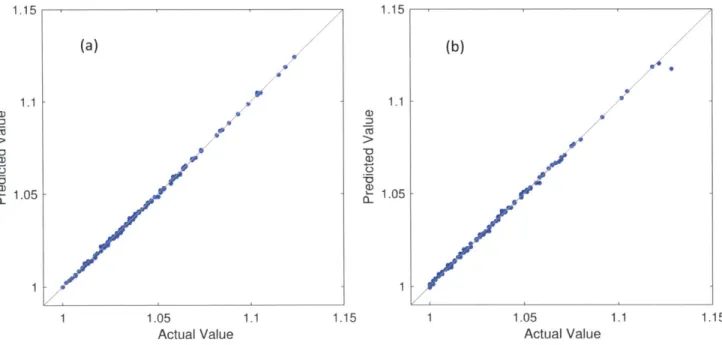
To finally assess the performance of the models, the completely separated test set was used. In order to better comprehend the results and the effect of a model, it was decided to normalize the performance score values (the output for the models) in a manner that the best performing design in the sampled data receives a score of 1 and the rest scale accordingly. For example, a score of 2 performs two times worse than the best design in the test set. A sample test set scatter plot of actual vs. predicted values can be seen in Figure 14 (it is put in context in the "Results" chapter). Apart from the scatter points, two dashed lines are plotted. Those represent the 10% error margins. The score of a point that lies on top of one of

based on the actual score. Naturally, all the points that lie between these lines have been predicted within a 10% accuracy (this representation is used in [10]). The solid grey line has a slope of 1 and as described in previous sections, represents the ideal exact prediction line. The scale on the two axes is the same.

1.6

1. 0/

/"0

1 1.1 1.2 1.3 1.4 1.5 1.6

Actual Value

Figure 14: Sample renormalized scatter plot (model: NN)

3.4 Sampling

The first step of any surrogate modelling framework is sampling. It refers to the gathering of a finite number of samples of design space parameters (explanatory variables) with the corresponding objective value (performance measure) for each of those samples. Those samples will be separated into training, validation and test sets for the model development phase.

3.4.1 Grasshopper sampling

For the case studies in the present thesis, the Rhinoceros software [39] was used along with the Grasshopper plugin [40] to generate the parametric design models as well as the objectives. For this reason, a sampling tool was developed for Rhino/Grasshopper since the existing ones were not deemed satisfactory.

The tool includes the following features: Sampling design space (Figure 15)

" Random

-

" Latin hypercube SEvaluating sample objectives

Random 0 0 -0 0 1 0.8 0 0.6-0.4 0 0 0 0.21 _ .2_. 0 0 0.2 0.4 0.6 0.8 1 0 S0 0 0.2

Grid Latin hypercube

0.8 * 0 0 0.6 * * * 0.4 0.2 01 0.4 0.6 0.8 1 0 0.2 0.4 0.6 0.8 1

Figure 15: Sampling plans

The three most common sampling plans included in the GH sampling tool are outlined schematically in Figure 15 for 16 samples in two dimensions in the [0,1] range.

The random scheme in this case refers to sampling uniformly random numbers for each variable within a specified range. The grid scheme is very straightforward; the given range for each variable is broken into points with equal distances and then all the sample combinations of those points are taken. The fact that all the combinations have to be sampled, makes the sample size grow geometrically with the number of variables (dimensions) for a given number of equidistant points in each dimension. This is the major drawback of grid sampling. With random sampling, one can take fewer samples than with the grid but there is no guarantee that those samples are going to spread evenly in the design space. The Latin hypercube scheme is a solution to have an evenly spread collection of samples without necessarily having to sample a large number of designs as in the Grid. More details about the Latin hypercube algorithm can

be found in [41], which was one of the first papers to study it in depth. The sampling tool uses the following two existing plug-ins:

* GhPython

I

I

The input sampling parameters of the tool are: n: total number of samples

k: number of design variables

Sampling scheme: Random/Grid/Latin hypercube (Only one of the options should be "True")

Random seed: seed to initialize random number generator, for consistent results 0.8 0.6 0.2 0 1

-w-i-Initially, the sampling is performed for each variable in the range (0,1). There is the capability to impose specific scaling upper/lower bounds for each parameter individually.

The tool has the additional capability to store screenshots of each design sampled. This feature builds on the notion that the framework is to be used in conceptual design, where a visualization of each design is

of equal importance as the design parameter data themselves.

The screenshot feature has flexibility over the following parameters as also shown on Figure 16. File name: the prefix of the screenshot file names

Save directory path: the path to which the screenshots will be saved File extension: the extension of the file to save the screenshots

Figure 16:

Screenshot tool parameters

3.5 Design example

The first case study, introduced here to illustrate the methodology concepts presented in the following sections, examines a seven (7) bar truss, whose geometry is shown in Figure 17. This is the "initial" geometry of the problem.

lF 1 -100 kN 2.0 m 2.0 m X3 0 1 2 _{-1.0 m} 0 0 4.0 m 3.0 m 1.0 m 4.0 m 4.0 mn

I

Figure 17:

Seven bar truss topology and design

(Image from [13])

The variables of the problem are xl, x2 and x3 as shown (along with their bounds in Figure 17 [13]). This case study is for research purposes and the methodology is intended for more complicated problems where the structural and/or energy analysis has significant computational needs.

The variables examined were the horizontal - xi- and vertical - X2 - position of one node of the truss as shown in Fig.1 and also the vertical - X3 - position of the node that lies in the axis of symmetry of truss. It should be noted that the structure is constrained to be symmetric. The design space was sampled based on the three (3) nodal position variables and each design was analyzed for gravity loads (accounting for steel buckling as well, which enhances the nonlinear nature of the problem) and a structural score of the form IALi (where A is the section area and L the length of member i) was determined as the objective.

The above problem has been originally addressed and studied and the datasets generated by [13].

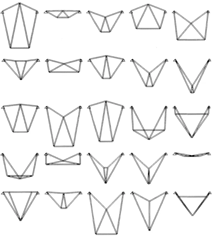
Using the developed GH sampling tool described above, data were collected to later fit approximation models from. In Figure 18, 25 designs produced are shown. Each design has a score associated with it, which is used to train an approximation model.

w-w

Figure 18: Design samples of Seven Bar truss generated by GH tool

VV Ak, "A'

VV