Potential and limitations of bioenergy options for low carbon transitions

HAL Id: hal-00866407

https://hal.archives-ouvertes.fr/hal-00866407

Preprint submitted on 30 Sep 2013

HAL is a multi-disciplinary open access

archive for the deposit and dissemination of

sci-entific research documents, whether they are

pub-lished or not. The documents may come from

teaching and research institutions in France or

abroad, or from public or private research centers.

L’archive ouverte pluridisciplinaire HAL, est

destinée au dépôt et à la diffusion de documents

scientifiques de niveau recherche, publiés ou non,

émanant des établissements d’enseignement et de

recherche français ou étrangers, des laboratoires

publics ou privés.

carbon transitions

Ruben Bibas, Aurélie Méjean

To cite this version:

Ruben Bibas, Aurélie Méjean. Potential and limitations of bioenergy options for low carbon

transi-tions. 2012. �hal-00866407�

C.I.R.E.D.

Centre International de Recherches sur l'Environnement et le Développement

ENPC

&

CNRS

(UMR

8568)

/

EHESS

/

AGROPARISTECH

/

CIRAD /

M

F

45 bis, avenue de la Belle Gabrielle

F-94736 Nogent sur Marne CEDEX

No 42-2012

Potential and limitations of bioenergy

options for low carbon transitions

Ruben Bibas

Aurélie Méjean

November 2012

Potential and limitations of bioenergy options for low carbon transitions

Abstract

Sustaining low CO2 emission pathways to 2100 may rely on electricity production from biomass. We analyze the effect of the availability of biomass resources and technologies with and without carbon capture and storage within a general equilibrium framework. Biomass technologies are introduced into the electricity module of the hybrid general equilibrium model Imaclim-R. We assess the robustness of this technology, with and without carbon capture and storage, as a way of reaching the RCP 3.7 stabilization target. The impact of a uniform CO2 tax on energy prices, investments and the structure of the electricity mix is examined. World GDP growth is affected by the absence of the CCS or biomass options, and biomass is shown to be a possible technological answer to the absence of CCS. As the use of biomass on a large scale might prove unsustainable, we illustrate early action as a strategy to reduce the need for biomass and enhance economic growth in the long term.

Keywords: General Equilibrium Model, Macro-economic Cost, Low Emission Objective, Electricity from Biomass, Carbon Capture and Storage, Negative Emissions.

o

Potentiel et limitations des options bioénergétiques dans les transitions faiblement carbonées

Résumé

La poursuite des trajectoires de faible émission de CO2 à l’horizon 2100 peut dépendre de la production d’électricité à partir de la biomasse. Nous analysons l’effet de la disponibilité des ressources et des technologies de la biomasse avec et sans captage et stockage de carbone dans un cadre d’équilibre général. Les technologies de la biomasse sont introduites dans le module électricité du modèle d’équilibre général Imaclim-R. Nous évaluons la robustesse de cette technologie avec et sans captage et stockage de carbone, comme moyen d’atteindre l’objectif de stabilisation RCP 3.7. L’impact d’une taxe carbone uniforme sur les prix de l’énergie, les investissements et la structure du mix électricité est examiné. La croissance du PIB mondial est affectée par l’absence des options du CSC ou de la biomasse, et la biomasse apparait comme une réponse technologique à l’absence du CSC. Dans la mesure où l’utilisation de la biomasse à grande échelle peut s’avérer comme non soutenable, nous illustrons l’action précoce comme une stratégie de réduction des besoins de biomasse et d’amélioration de la croissance économique à long terme.

Mots-clés : modèle d’équilibre général, coût macro-économique, objectif de faible émission, électricité issue de la biomasse, captage et stockage du carbone, émissions négatives.

transitions

Ruben Bibas

Aurélie Méjean

November 20, 2012

∗_{CIRED – International Research Center on Environment and Development, 45 bis, Avenue de la Belle Gabrielle, 94736} Nogent-sur-Marne, France. Corresponding author:

Contents

1 Introduction 4

2 Methods: the challenges of integrating bioenergy into energy-economy modeling 5

2.1 Reconciling top-down integration and bottom-up accuracy . . . 5

2.2 The hybrid model Imaclim-R: integrating bottom-up modules into a general equilibrium framework 6 2.2.1 Imaclim-R: an innovative macroeconomic framework . . . 6

2.2.2 Integrating biomass technologies into the electricity sector . . . 6

2.2.3 Integrating biomass use in the transportation sector . . . 7

2.3 Study protocol . . . 8

3 Results: the influence of contrasted technology assumptions 8 3.1 Decarbonizing the electricity sector . . . 8

3.2 The carbon tax profile . . . 9

3.3 Agricultural and electricity prices . . . 10

3.4 The macroeconomic costs of climate policies . . . 10

3.4.1 The profile of GDP losses . . . 10

3.4.2 Determinants of GDP losses . . . 11

4 Climate policy as a hedge against technological uncertainty: debating early action 12 4.1 Biomass production and land competition . . . 12

4.2 Early action as a way to reduce bioenergy and land requirements . . . 12

5 Conclusion 14 Acknowledgements 14 Bibliography 14

Appendices

18

A.2 Biomass supply curve for biofuel production . . . 18

A.3 All biomass types . . . 19

B Electricity technologies characteristics 20 C Matching between EMF27 and paper scenarios 22 D Emissions trajectories 23 D.1 Emissions trajectories for EMF27 study . . . 23

D.2 Emissions trajectories for additional discussion case . . . 23

F Electricity demand 25

G Electricity mixes 26

H Investments 27

I Energy shares in production costs 28

J Consumption Price Index 29

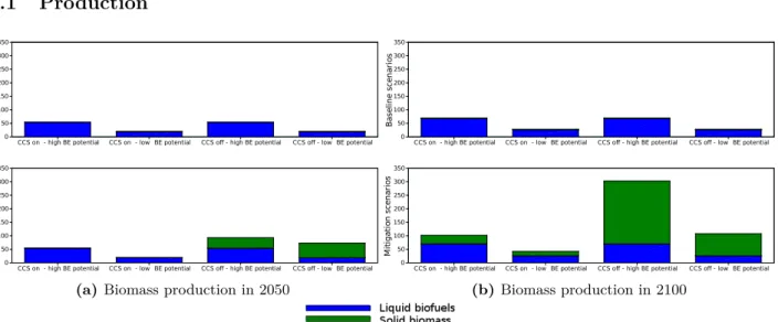
K Biomass 30

K.1 Production . . . 30 K.2 Negative emissions from BECCS . . . 30

L Sectoral CO2 emissions abatement 31

M Prices of goods 32

Abstract

Sustaining low CO2 emission pathways to 2100 may rely on electricity production from biomass. We

analyze the effect of the availability of biomass resources and technologies with and without carbon capture and storage within a general equilibrium framework. Biomass technologies are introduced into the electricity module of the hybrid general equilibrium model Imaclim-R. We assess the robustness of this technology, with and without carbon capture and storage, as a way of reaching the RCP 3.7 stabilization target. The impact of a uniform CO2 tax on energy prices, investments and the structure of the electricity mix is examined.

World GDP growth is affected by the absence of the CCS or biomass options, and biomass is shown to be a possible technological answer to the absence of CCS. As the use of biomass on a large scale might prove unsustainable, we illustrate early action as a strategy to reduce the need for biomass and enhance economic growth in the long term.

Keywords: general equilibrium model ; macro-economic cost ; low emission objective ; electricity from

biomass ; carbon capture and storage ; negative emissions.

1

Introduction

Recent studies suggest that energy produced from biomass may play a significant role for reaching ambitious

climate stabilization objectives (van Vuuren et al.,2010). Bioenergy is usually considered a source of sustainable,

clean energy for two crucial uses: (i) transport as a substitute for oil and (ii) electricity as a substitute for fossil fuels into conventional thermal power plants.

Furthermore, the enthusiasm surrounding bioenergy largely relates to the expectation that it may allow

negative CO2 emissions when combined with carbon capture and storage technologies (CCS). Indeed, reaching

low climate stabilization objectives may require net negative emissions towards the end of the century (Fisher

et al., 2007). Negative CO2 emissions can be achieved through direct or indirect CO2 removal methods, for

instance by enhancing land carbon sinks through land use management1_{, natural weathering processes or the}

oceanic uptake of CO2, by the direct engineered capture of CO2 from ambient air or by using biomass for

carbon sequestration (The Royal Society, 2009). In the latter case, CO2 is removed from the atmosphere

through photosynthesis as vegetation grows, and this carbon can be sequestered in the long term by cutting and

burying the grown biomass (Metzger and Benford,2001) or by combining energy production from biomass and

carbon capture and storage (BECCS2_{). While they remain very uncertain and controversial, these technologies}

are often expected to play quite a significant part in the reduction effort in the long term. In fact, many modeling exercises have shown that negative emissions produced through the deployment of CCS in combination with

bioenergy could significantly reduce the cost of climate mitigation (Azar et al.,2006;Wise et al.,2009;Edenhofer

et al.,2010;Luckow et al.,2010;van Vuuren et al.,2010).

However, significant uncertainties remain on the economic and environmental impacts of large scale

pro-duction of biomass for energy purposes, in particular as regards land competition, agricultural prices and CO2

emissions from land-use change (Sands and Leimbach,2003;Fisher et al.,2007). The large-scale deployment of

carbon capture and storage technologies has yet to be proved technically and economically feasible and large

uncertainties remain on the size of geological storage capacity and possible leakage from those reservoirs (Metz

et al.,2005). The potential unsustainability of these technologies leads to a great uncertainty on the bioenergy and CCS potentials.

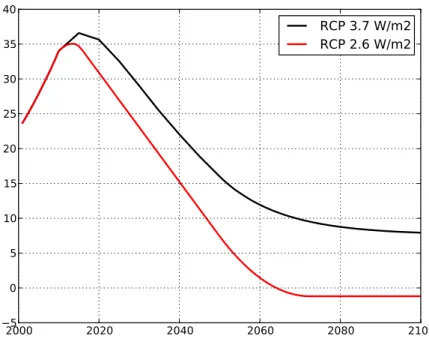
The emissions constraint of the RCP 2.6 scenario requires net negative emissions after 2070. This very low stabilization scenario thus cannot be solved without BECCS technologies in most models. The aim of our study is to reveal the impact of the availability of biomass resources and CCS on the cost of climate mitigation. Our study focuses on RCP 3.7 climate scenarios, for which global net negative emissions are not strictly required.

Bioenergy use in EMF27 scenarios can reach 300 EJ of grown biomass per year. Depending on crucial assumptions on yields, this amount of biomass could require up to several GHa of additional land. With approximately 13 GHa of emerged land available, of which about a third are forests (5 GHa) and another third is agricultural land (4 GHa), the additional stress on land use may prove unsustainable in terms of biodiversity loss, local environmental impacts (air, water and soil quality), local land rights, rising food prices and greenhouse

gas emissions from direct and indirect land-use change (Gallagher et al.,2008). This paper examines the role of

bioenergy for low carbon stabilization targets and revisits the underlying, sometimes controversial, assumptions that models embody in terms of biomass availability. To that end, we examine mitigation scenarios, contrasted in their assumptions on biomass and CCS availability.

1_{Land-use management includes reforestation and afforestation.}

2 _{BECCS stands for Bio-Energy with Carbon Capture and Storage. This term was first introduced in (Azar et al.,2006) and} (Fisher et al.,2007).

In order to assess the implications of these assumptions from both an energy and economic perspectives, our modelling framework must integrate specific information on the electricity and liquid fuels sectors within a consistent economic framework, including the competition with other agricultural products and energy goods. Such a setting is needed to reveal the impacts and interactions of BECCS with upstream and downstream economic activities. Therefore, this study requires a Computable General Equilibrium (CGE) model and a framework including a bottom-up electricity supply model accounting for the diversity of technologies and fuels available and sectoral specificities of electricity supply, such as capacity vintages and investment crowding-out. In addition, biomass production and use result from the interaction of energy demand from all sectors, competition between liquid fuels and with agricultural goods. In consequence, the sectoral bottom-up modules should interact with the CGE macroeconomic framework to assess the macroeconomic effects of climate and energy policies.

The paper is organised as follows. Section 2 discusses the gap in the literature in terms of integrated assess-ment of electricity production, land-use and the economy and reveals the required model features prescribing specific model forms. Drawing from the discussion on resource availability, section 3 presents scenarios that challenge the idea that large biomass resources are needed to achieve ambitious mitigation targets. The sce-narios examine the complementarity of bioenergy and CCS, revisiting the synergies between both technologies.

The results show the influence of bioenergy and CCS on (i) the CO2 tax, (ii) the electricity sector, and (iii) the

prices of electricity and agriculture, in order to elicit the determinants of macroeconomic costs and explain the time profile of mitigation costs. Section 4 discusses the impact of bioenergy use on land competition and the role of the timing of the efforts to limit the need for BECCS and biomass resources. Section 5 concludes on the role of bioenergy as a robust mitigation strategy.

2

Methods: the challenges of integrating bioenergy into

energy-economy modeling

2.1

Reconciling top-down integration and bottom-up accuracy

The interactions between the economy, energy sectors, and climate policies are traditionally studied using bottom-up approaches, often in partial equilibrium, or using top-down energy-economy models which represent energy in an aggregate manner.

Top-down models usually rely on aggregate production functions (Solow, 1956). Conventional production

functions describe available techniques and the technical constraints ruling the economy (Berndt and Wood,

1975; Jorgenson and Fraumeni, 1981). However, the aggregate representation of a continuous space of tech-nologies via production functions is only theoretically justified near the equilibrium, and the use of constant elasticities of substitution may lead to incorrectly exceed feasible technical limits in the case of large departures

from the reference equilibrium (McFarland et al., 2004; Ghersi and Hourcade, 2006). Moreover, short-term

econometric analyses have shown that modeling exercises can better reproduce the observed magnitude of the economic effect of energy price variations if they include (i) mark-up pricing to capture market imperfections (Rotemberg and Woodford,1996) ; (ii) putty-clay descriptions of technologies translating the inertia of capital

stock renewal (Atkeson and Kehoe, 1999) ; (iii) partial utilization rate of installed production capacities due

to the limited substitution between capital and energy (Finn, 2000) ; and (iv) imperfect expectations (Fisher

et al.,2007;Downing et al.,2005).

Bottom-up approaches represent sectoral mechanisms, which should include some specific features. The com-bination of inertia and imperfect foresight may cause excess or shortage of supply, creating market disequilibria

in the long-run (Sterman,2000;Rostow,1993). This, along with the trend towards power sector liberalization,

calls for abandoning perfect foresight and using adaptive simulation models, as illustrated in (Olsina et al.,

2006). Market disequilibria create business cycles in the electricity sector (Bunn and Larsen,1992;Ford,1999)

and econometrically estimated byArango and Larsen(2011). Also, electricity must be considered as a “derived

demand”, that is to say not providing utility in itself, but allowing for the use of other goods or services which

directly provide utility (Taylor, 1975). The representation of the electricity sector requires the explicit and

detailed description of technologies (Bhattacharyya, 1996). This high level of details requires the description

of load demand curves (especially peak and non-peak) and short and long term demand, using for instance

short-term marginal cost pricing as well as differentiated prices for different users (Taylor, 1975). Moreover,

the representation of inertia in the sector is indispensable, whether it be in the end-use sectors (Silk and Joutz,

The difficulty of transposing micro-economic mechanisms at the aggregate level can be overcome using

bottom-up engineering information as a way to enhance the technological realism of production functions (

Mc-Farland et al., 2004). Specific interactions between the electricity sector and the CGE framework should be considered: (i) the impact of energy prices on electricity production ; (ii) the substitution between electricity and other energies in end-use sectors (households and firms) and the wider cross-sectoral effect of electricity production on fuels prices ; (iii) the very capital intensive nature of electricity production, which may lead to crowding out effects on investment, as the electricity sector takes precedence over the other productive sectors given the “essential good” nature of electricity; (iv) the dynamics of electricity demand.

The CGE model Imaclim-R aims at bridging the gap between top-down and bottom-up approaches, as it incorporates bottom-up modules into a CGE framework.

2.2

The hybrid model Imaclim-R: integrating bottom-up modules into a general

equilibrium framework

2.2.1 Imaclim-R: an innovative macroeconomic framework

Imaclim-R World is a recursive, dynamic, multi-region and multi-sector hybrid CGE model (Waisman

et al., 2012a)3_{. It is calibrated for the 2001 base year by modifying the set of balanced input-output tables}

provided by the GTAP-6 dataset (Dimaranan, 2006) to make them fully compatible with 2001 IEA energy

balances (in Mtoe) and data on passengers’ mobility (in passenger-km) from Schafer and Victor(2000).

This hybrid model integrates bottom-up engineering modules with explicit technologies into a top-down CGE macroeconomic framework with capital accumulation. Imaclim-R thus creates technical scenarios consistent

with an economic trajectory where growth is based on explicit technical content. “Hybrid matrices” (Hourcade

et al., 2006) ensure a description of the economy in consistent money values and physical quantities (Sands et al., 2005). The dual description represents the material and technical content of production processes and allows for abandoning standard aggregate production functions, which have intrinsic limitations in case of large

departures from the reference equilibrium (Frondel and Schmidt, 2002). The absence of a formal production

function is compensated for by a recursive structure that allows a systematic exchange of information between an annual macroeconomic equilibrium module and technology-rich dynamic modules.

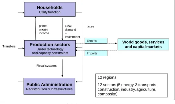
The annual static equilibrium (figure 9a) determines relative prices, wages, labour, value, physical flows, capacity utilization, profit rates and savings at date t as a result of short term equilibrium conditions between demand and supply on goods, capital and labor markets. It is calculated assuming Leontief production functions with fixed intermediate consumption and labor inputs, decreasing static returns caused by higher labor costs

at high utilization rate of production capacities (Corrado and Mattey,1997) and fixed mark-up in non-energy

sectors.

The dynamic modules (figure 9b), including demography, capital dynamics and sector-specific modules assess the reaction of technical systems to the economic values of previous static equilibria and send back this information to the static module in the form of new input-output coefficients to calculate the next yearly equilibrium. Each year, technical choices are flexible but modify only at the margin the input-output coefficients and labor productivity embodied in existing equipment resulting from past technical choices. This general putty-clay assumption is essential to represent the inertia in technical systems and the role of volatility in economic signals. Among the dynamic modules, most energy sectors are represented via stylized bottom-up models, including power generation.

In mitigation scenarios, the CO2 trajectory is a model input and the CO2 price is each year calculated

endogenously by the model. As Imaclim-R is a recursive simulation model (and not an optimization model), the carbon price is not the result of the action of a social planner but of the decisions of multiple actors in a second best world. Imaclim-R thus simulates exploratory scenarios.

2.2.2 Integrating biomass technologies into the electricity sector

The electricity sector was historically the focus of important modeling efforts. This sector was often centrally planned, leading to wide developments of bottom-up optimization models. It is very capital-intensive, which

3_{The 12 regions are USA, Canada, Europe, OECD Pacific, Former Soviet Union, China, India, Brazil, Middle-East, Africa, rest} of Asia, rest of Latin America. The 12 sectors are divided as follows: three primary energy sectors (Coal, Oil, Gas), two transformed energy sectors (Liquid fuels, Electricity), three transport sectors (Air, Water, Terrestrial Transport) and four productive sectors (Construction, Agriculture, Industry, Services).

raises short-term and long-term macroeconomic issues, especially when ambitious climate policies could increase capital costs (e.g. uncertainties on CCS, shifts to renewables). The specificities of the electricity sector call for specific model features. Electricity cannot be easily stored and a constant balance between power available on the grid and power demanded by final uses (the load) must be met at all times. Production must therefore adapt to major daily and seasonal fluctuations of demand. Load curves, technology specificities, capital intensity, capacity vintages and imperfect foresight should thus be modeled, as they determine investment decisions.

The electricity supply module in Imaclim-R tracks production capacities over time, thus incorporating the inertia and path-dependency of the system. Investment decisions are made to meet future demand while minimizing long-term marginal production costs. In order to acieve this optimal mix, expectations are formed

ten years forward for demand, fuel costs, and the CO2tax. The profitability of production technologies depends

on annual operating time, which derives from short-term marginal cost minimization. The model covers the heterogeneity of fixed and variable costs for each technology and operational constraints. Indeed, both long term investment choices and choices concerning putting existing capacities into operation depend on the load curve. The minimization of the discrepancy between installed capacities and the expected optimal mix triggers investments to reach this optimal mix over 10 years. This process of optimal planning with imperfect foresight occurs every year and expectations adapt to changes in prices and demand.

The representation of technology specifications contrasts with aggregated macroeconomic functions. How-ever, the choice of power technologies cannot simply be made using an aggregated merit-order: the representation of investment choices based upon capacity vintages, imperfect foresight and load curves is essential. Investment decisions are taken for 26 technologies (15 conventional including coal, gas – and oil-fired, nuclear and hydro and 11 renewables including biomass-fired thermal plants, with or without CCS). The share of each technology in the optimal mix of producing capacities results from a competition among available technologies depending on their mean production costs for yearly production durations using a logit form. That is, competition is differentiated to account for the fact that the capacity is expected to meet peak or base load demand. In addition, other constraints are taken into account (e.g. social acceptability, investment risk, size of production units, market structure) via ‘intangible” costs, which translate in economic terms the constraints faced when making investment decisions, however not inducing any money transfer further along during production.

Our study focuses on the role of biomass to decarbonise the economy. Following the modeling specifications

of Image described by Hoogwijk et al. (2009), land resources available for biomass production dedicated to

power generation are restricted to abandoned agricultural land and rest land. The most conservative assumption

of the four SRES scenarios (scenario A2 from Nakicenovic et al.(2000)) was retained for the maximum global

biomass production (302 EJ/year) in 2050 (cf. section A.1). Biomass-fuelled power plants are characterized by a cost structure and technical performances similar to coal-fuelled plants. However, the resource price is different: in all EMF27 scenarios, biomass is on average more than 7 times more expensive than coal and 4 times more expensive than gas. Only very high carbon taxes can make biomass competitive with fossil fuels. Biomass use greatly modifies the input-output structure of the economy, as electricity generation relies on agricultural products (including forests) instead of mineral resources, thus shifting the production from imported fossil fuels to domestic agricultural goods.

The outstanding issue of who shall benefit from the carbon tax combined with negative emissions, which corresponds to a direct subsidy, is debatable. The alternative lies between farmers and electricity producers:

farmers capture atmospheric CO2into biomass and electricity producers store it using CCS technologies. While

electricity producers would probably not implement this technology unless the additional cost compared to conventional fuels is paid, farmers would not choose to grow bioenergy crops without strong incentives. Our modeling choice here is neutral, as farmers are paid by electricity producers at the level of their production costs (including a fixed profit) while electricity producers receive the subsidy on the amount of produced BECCS. However, they have to pay an equivalent amount, distributed on the final electricity production, and passed through to consumers, which makes this subsidy neutral for governments. This question should be addressed in further work with a specific bottom-up module of land-use representing land rents.

2.2.3 Integrating biomass use in the transportation sector

The availability of biomass may also greatly impact the decarbonisation of the transportation sector. Tech-nology (carbon intensity of fuels and energy intensity of mobility) and behavioral (mobility volume and modal

shares) determinants drive transport emissions (Chapman,2007;Schäfer,2012). Imaclim-R adopts an explicit

representation of fuel and transport technologies and passenger and freight mobility (Waisman et al.,2012b).

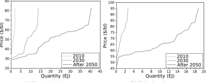
Biofuel penetration in liquid fuel markets depends on their availability and their competitiveness with oil-based fuels. The constraint on the availability of agricultural land is thus captured by a threshold value on production. Biofuels supply curves (figure 5) define the maximum amount of biofuels that can penetrate the market at a given date and for a given price of refined oil products (including taxes). They are calibrated on sectoral

modeling results (International Energy Agency and Organisation for Economic Co-operation and Development,

2006). The penetration of biofuels is calculated by equalling their marginal production cost and the price of

conventional refined oil. At each date, the market share of biofuels is therefore an increasing function of oil prices.

In addition to the standard representation of transport fuels and technologies, Imaclim-R explicitly accounts for the behavioural determinants of mobility which drive demand for transport: constrained mobility needs imposed by the spatial organization of residence and production (i.e. commuting), modal choices triggered

by available infrastructure and the freight transport intensity of production (Waisman et al., 2012b). First,

households maximize utility under budget and time constraints, which affects their decisions about mobility volume and modes. This allows to capture the rebound effect of energy efficiency improvements on mobility, the induction effect of infrastructure deployment on mobility demand, the modal split, and the constraint imposed by the location of firms and households on mobility needs. Second, freight mobility in a given mode (air, water, terrestrial) is assumed to increase linearly with production volumes. This dependence evolves over time to capture the changes in the energy efficiency of freight vehicles, the organization of the production and

distribution processes and the modal split. Waisman et al. (2012b) demonstrate that the implementation of

measures inducing a shift towards low-carbon transport modes and a decoupling of mobility needs from economic activity reduces the carbon tax levels necessary to reach a given climate target.

2.3

Study protocol

Table 1: Technology and resource scenarios

CCS availability _{High (300EJ/year) Low (100 EJ/year)}Biomass availability

On (1) (2)

Off (3) (4)

Four technology scenarios are considered in the results section (section 3), according to the availability of the CCS technology (on or off) and the availability of biomass resources (300 or 100 EJ/year), leading to 4 technological possible backgrounds. This set-up is used to estimate the costs of reaching a RCP 3.7 target with

a carbon price as the sole instrument over the 2010-2100 period. Table 1 summarizes the scenarios4_.

3

Results: the influence of contrasted technology assumptions

3.1

Decarbonizing the electricity sector

The constraint on CO2 emissions triggers the fast decarbonization of the electricity sector (more than 85%

abatement by 2050, cf. appendix G). Electricity production from coal and gas without CCS is phased out by 2050 in both scenarios where CCS is available.

While the availability of biomass resources does not influence the date of entry of BECCS, the availability of CCS delays the penetration of bioenergy from 2040 (without CCS) to 2060 (with CCS). This contrasts with

optimization results under perfect foresight, e.g. (Magne et al.,2010), where an earlier date of entry of BECCS

is required in the low resource case to achieve sufficient abatement. Our result is explained by the fact that Imaclim-R is not intertemporally optimizing and runs under imperfect foresight.

The availability of CCS greatly influences the nature of the electricity mix, as it locks the electricity system into a path dominated by fossil fuels (scenarios 1 and 2), explaining the need for a higher carbon price for bioenergy to penetrate the mix. The unavailability of CCS induces a wider deployment of nuclear energy (e.g.

scenario 3 compared to scenario 1)5_.

4_{For matching, cf. appendix C: table 4 maps the matching between the scenarios presented in this paper and the overall EMF27} study.

5_{In a scenario without CCS, the decarbonisation of electricity largely relies on the deployment of nuclear technologies, because} the share of intermittent renewables is constrained.

2010 2020 2030 2040 2050 0 100 200 300 400 500 600 700 800 High biomass CCS on (1)

High biomass CCS off (3) Low biomass CCS on (2)Low biomass CCS off (4)

(a) Short term

2050 2060 2070 2080 2090 2100 500 600 700 800 900 1000 1100 1200 1300 High biomass CCS on (1)

High biomass CCS off (3) Low biomass CCS on (2)Low biomass CCS off (4)

(b) Long term Figure 1: World CO2 tax to reach the RCP 3.7 target in each scenario

Technology options impact the evolution of investments in the agricultural and electricity sectors (ap-pendix H). When CCS is available, the investments in the electricity sector are similar to those of the baseline: the increase consistently follows demand increases across scenarios (appendix F). However, the extensive use of biomass triggers the increase in investment in the second half of the century, which doubles in 2100 to meet demand. These investment needs and supply constraints build up price increases (appendix M). When CCS is unavailable, electricity production resorts to nuclear, which requires large investment compared to fossil fuel power plants, leading to the doubling of investment in the electricity sector in mitigation scenarios. In paral-lel, the unavailability of CCS tightens the agriculture market: supply investments more than double to meet demand (appendix K).

The additional investments in both sectors lead to a crowding-out of investment in other productive sectors, which partly explains the losses between 2020 and 2040 (electricity investments to replace CCS) and after 2070 (impact of low biomass availability on the agricultural sector). As the electricity sector is a major emitting sector, its dynamics drive the carbon tax.

3.2

The carbon tax profile

A CO2 tax increases the cost of energy for all sectors, and Imaclim-R endogenously determines the tax

to be imposed on CO2 emissions to meet the emissions constraint. This tax is paid for by energy consumers

when emitting CO2from energy use, and the increase in prices is ultimately paid for by final consumers as it is

passed through the input-output table that represents the structure of the economy. The resulting tax profiles (figure 1) reveal two price dynamics. These dynamics are due to the interaction between emissions constraints (emissions decrease faster between 2010 and 2050) and different sectoral abatement profiles in a given economic context (growth, population, resources). Contrary to the usual atemporal representation of abatement curves, the bottom-up technical modules encompass a time dimension that incorporates technical inertia and imperfect foresight as a direct determinant of abatement.

In the short-term (until 2050 – figure 1a), the constraint is reached more easily when CCS and large biomass ressources are available. The relaxation of the constraint on technologies translates into a lower carbon tax. Imaclim-R carbon price results from finding the price of carbon to abate emissions and match the constraint on a yearly basis. It corresponds to the shadow value of an annual optimization problem, or to the tax needed to abate the last ton of carbon to meet the constraint. Contrary to intertemporal optimization models, the carbon price in Imaclim-R is an instantaneous (and path-dependent) marginal abatement cost. This interpretation of the carbon price explains why removing some technical options translates into higher prices. In the studied scenarios, the unavailability of CCS is the main driver of the increase in carbon prices as CCS is technically available and cost-competitive at this temporal horizon. The increase due to a lower biomass potential is smaller (as biofuel penetration is constrained and woody biomass is not competitive until 2040 in the optimistic scenario), but the same reasoning applies: removing an option increases the immediate marginal abatement cost.

In the long-term (between 2050 and 2100), carbon prices (figure 1b) oscillate around 913$/tCO26. The

availability of short-term options relaxes the required efforts but comes at a price in the long-run: the average

carbon tax reaches 948$/tCO2with CCS and 878$/tCO2without CCS. By contrast, when some decarbonisation

options are unavailable, a high carbon tax in the short-term triggers energy efficiency mechanisms, resulting in a much lower tax in the longer term (all curves cross in 2053). This instantaneous stiffening of the constraint followed by a relaxation of the constraint is mostly due to inertia in installed productive capital.

3.3

Agricultural and electricity prices

Carbon prices and technology options impact the prices of electricity and agricultural and composite goods (cf. appendix M). Every scenario shows an increase in electricity prices in the short term (figure 17a), due to the increase in fossil fuels prices. The carbon tax weighs heavily for about 30 years, which corresponds to the time of renewal of electric capacities. CCS allows for cheaper electricity in the short run, but induce a lock-in in fossil fuels, leading to a slight rise in price after 2060 due to the increase of fossil fuels prices. Without CCS, electricity production relies slightly longer on gas and then heavily on nuclear. After 2040, the electricity system has adapted to a heavy carbon constraint and prices return to baseline levels.

BECCS amplifies this price increase after 2060: as biomass prices increase when supply curves saturate at the end of the century, the high price of this fuel weighs on electricity prices. When CCS is unavailable, the early move away from fossil fuels serves as a long term hedge against fossil fuel price increases, and electricity prices are lower after 2040 in these scenarios.

Biomass use greatly impacts the agricultural sector (figure 17b). In the baseline scenario, biofuels for transport are used at the end of the century after the peak oil, but still in low quantities. When biomass is highly available, hence at a relatively low price for high resource use, the agriculture price increase by 8%. When biomass potential is low, the higher price of biomass pusges up the price of agricultural commodities (20% increase in 2100 compared to baseline). A formal feedback of land use on land rents would enhance the adverse effect of bioenergy production on agricultural prices and would further question the sustainability of scenarios with a widespread use of bioenergy.

3.4

The macroeconomic costs of climate policies

3.4.1 The profile of GDP losses

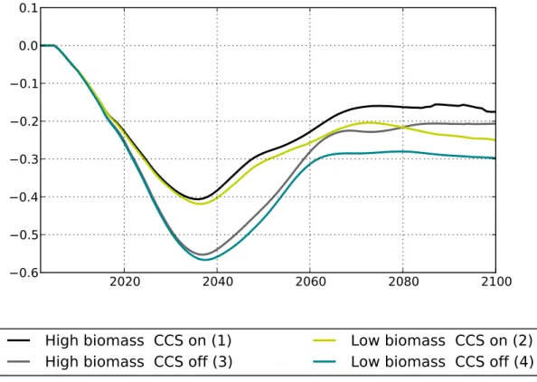
Figure 2 shows the macroeconomic cost profile of a RCP 3.7 climate constraint under four technology and resource scenarios. The costs are shown as the difference in average GDP growth rate between the no climate

policy baseline (i.e. under no climate constraint) and each of the four scenarios under climate constraint7_{. This}

indicator translates costs in terms of growth losses over the period8_.

In the short term, the availability of biomass resources has little influence on costs. In the longer term however, the size of biomass resources plays a crucial role, especially when CCS is not an option. Before

year 2050, the slower economic growth9 _{in the climate scenario is solely explained by the unavailability of the}

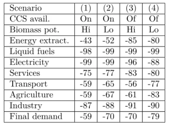
CCS technology. After 2050 the unavailability of CCS combined with the low availability of biomass resources induces the highest costs. Without CCS, the larger availability of biomass greatly mitigates these costs: the use of biomass then becomes one of the few possible options to produce low-carbon electricity. It is interesting to note the partial economic recovery between 2040 and 2070 in the scenarios without CCS, due to the early transition away from fossil fuels use. While the economic recovery continues after 2070 in the high resource scenario, the low availability of biomass for electricity production hampers growth after that date. Electricity from biomass, combined with biofuels availability for transport, in scenario 3, display a final level of losses lower than the scenario with CCS with a low availability of biomass (scenario 2).

The contribution of electricity to abatement is higher with CCS (especially in the short term) (appendix L). A decarbonization of 98% of the electricity sector (vs. 86% without CCS), allows for the displacement of the

6 _{The actual value considerably varies for other technical, economic and environmental assumptions.}

7_{The costs correspond to the average loss of annual growth rate between the beginning of the period and the considered date.} -0.3% in 2060 therefore means a decrease in annual growth rate for the period 2010-2060.

8_{This indicator smoothes shocks and translates growth losses on a yearly scale which is understandable regardless of the initial} level and economic context. This synthetic indicator of the state of growth over the period at a given date reveals the arbitrage between short and long-term costs.

9_{Note that the negative sign of the difference in growth rates means that economic growth is higher in the reference scenario} than in the climate policy scenario. However, growth remains positive.

2020

2040

2060

2080

2100

0.6

0.5

0.4

0.3

0.2

0.1

0.0

0.1

High biomass CCS on (1)

High biomass CCS off (3)

Low biomass CCS on (2)

Low biomass CCS off (4)

Figure 2: Macroeconomic cost profile of the RCP 3.7 climate policy under four scenarios

constraint from transport (33% vs. 53%) and final demand (37% vs. 47%). The availability of biomass also induces a greater contribution of the electricity sector in overall abatement, relaxing the constraint on transport and final demand. Technology availability assumptions shift the constraint and alter sectoral abatement costs. In conclusion, a constraint on either option – biomass or CCS – leads to a significant increase in costs. With any of the two options available, losses are reduced compared to the scenario with both options unavailable. The caveat is that CCS allows for a reduction in economic losses in the mid-term rather than in the long-term, whereas bioenergy does not prevent short and mid-term losses but allows to come very close to the cost level of the optimistic scenario, when both options are available. These results illustrate the strong complementarity of these options to prevent large economic losses in the short, medium and long term.

3.4.2 Determinants of GDP losses

Even in the optimistic technology scenarios, the cost of reaching the RCP 3.7 climate stabilization objective is significant. The magnitude of the cost as revealed by the modeling exercise can be explained by the interaction between the energy-economy system and the choice of policy instruments for climate mitigation within the modeling framework of Imaclim-R. Imaclim-R models market imperfections, inertia, short-run adjustments constraints and imperfect expectations, which may induce higher costs than in the case of inter-temporal

optimization with perfect foresight (Fisher et al.,2007). The sole policy instrument used in the EMF27 study is

a uniform CO2 tax imposed on CO2emissions from fossil fuels use. A single price signal may be suited to

first-best modeling frameworks. However, in the case of imperfect markets (including imperfect labor markets) and imperfect foresight, the absence of accompanying instruments such as policies inducing a shift in investments

towards public transportation infrastructure Waisman et al.(2012a), labor policiesGuivarch et al.(2011) may

partly explain the high macroeconomic cost of climate mitigation.

The level of the CO2tax impacts the share of energy in all sectors. Economic growth is driven by two major

indicators of economic activity: industrial production costs and consumer prices, so the analysis focuses on the impact of the carbon tax on the industrial sector and on households in the optimistic technology case (scenario 1).

In the short to medium term, the share of energy in total production costs (appendix I) is pushed up by the tax imposed on emissions from fossil fuels in the mitigation scenario. The magnitude and timeframe of this increase strongly depend on scenario assumptions. This trend is reversed in the very long term as low-carbon technologies take a larger share in the energy mix and become cheaper through technological learning. High carbon prices in the first half of the period induce a structural change in industry towards less carbon intensive processes. This shift is visible from 2060 with the steep decrease in the share of energy costs in total industrial production costs. The delay of this decrease is explained by the low rate of depreciation of productive capital in the industrial sector.

A second major determinant of the macroeconomic cost of climate policies is the effect of the CO2 tax on

consumer prices. Consumer prices reflect the increase of energy costs through the increase in the price of goods that follow the increase in energy prices. The inter-sectoral impacts follow the input-output structure of the economy, leading to a generalized increase in consumer prices for all goods. This effect is revealed by the level of

the consumption price index in the baseline and climate policy scenarios (appendix J). The CO2tax pushes up

the consumption price index in the short term. However, early carbon pricing accelerates learning in low-carbon technologies and reduces oil demand in the short term, thereby reducing the adverse effect of the peak oil and

soaring oil prices in the medium term (Rozenberg et al.,2010;Waisman et al.,2012a). The consumption price

index steeply increases after 2050, which coincides with the deployment of electricity production from biomass. This result is partly explained by the increase in agricultural prices due to the wider use of biomass for energy purposes. After 2070 the consumption price index is largely driven by transportation costs due to the restricted number of options available for low-carbon transport.

4

Climate policy as a hedge against technological uncertainty:

de-bating early action

4.1

Biomass production and land competition

Although bioenergy could play a crucial role in climate change mitigation, several issues remain. Indeed, the large scale production of biomass for energy may generate emissions from deforestation and agricultural intensification and adversely impact food prices. The uncertainty on yield impvrovements causes uncertainty on

sustainable bioenergy availability. Haberl et al.(2010) suggests that managed forests expect the highest yields

in 2050: 149 GJ/ha/year, with a reported variability between 69 and 600 GJ/ha/year. With this assumption, the production of 300 EJ/year of biomass worldwide would require a land area of 2.01 Gha, corresponding to about 15% of total land area. The purpose here is not to discuss the value itself, but rather to understand its impacts on the economy-energy system and find ways to reduce bioenergy (and land) requirement considering the possible unsustainability of bioenergy production. Beside the number itself, the order of magnitude suggests an unsustainable level of biomass use. The influence of the increasing use of biomass energy on agricultural markets is captured through the price of agricultural goods. The explicit interaction between land rents, land competition and farming production choices would likely increase agricultural prices, hence increasing mitigation

costs10_.

Moreover, the sustainability of biomass resource use should be assessed when reporting and accounting

for emissions (International Energy Agency, 2011). Biomass for electricity production may be produced from

unsustainable sources in non-Annex I countries but used in Annex I countries and accounted for as a sustainable fuel. In order to address this issue, biomass for electricity is assumed to grow on abandoned land (i.e. not forest), which means that the figure used for available land area used to grow biomass for energy purposes should assume no deforestation. This further raises the issue of expected yield improvements, as the available area of abandoned land may not be sufficient to meet demand for bioenergy.

4.2

Early action as a way to reduce bioenergy and land requirements

Mitigation costs are very sensitive to often controversial technology assumptions, whether related to the technical availability of CCS or land-use impacts of bioenergy production. In particular, even in scenarios where nuclear largely deploys, the amount of biomass necessary for energy production purposes commands unsustainable land use, up to 1.48 Gha. The great impact of the size of biomass resources on mitigation costs raises the question of the realism of the assumptions made in terms of technologies, land use and production

5 10 15 20 25 30 35 40 2010 2020 2030 2040 2050 2060 2070 2080 2090 2100

(a) Alternative emissions trajectories constraints (GtCO2)

-1.6 -1.4 -1.2 -1.0 -0.8 -0.6 -0.4 -0.2 -0.0 2010 2020 2030 2040 2050 2060 2070 2080 2090 2100

(b) Resulting negative emissions (GtCO2)

0 100 200 300 400 500 600 2010 2020 2030 2040 2050 2060 2070 2080 2090 2100 (c) CO2 tax (2005 USD) -12 -10 -8 -6 -4 -2 0 2 2010 2020 2030 2040 2050 2060 2070 2080 2090 2100

(d) GDP losses (% MER real, difference w.r.t. baseline) Figure 3: Discussion of early action

yields, hence the question of which strategies should be implemented in order to hedge against uncertainties about supply side options. In order to go beyond the mere technological assessment, we examine policy options that may help overcome the cost impacts of a constraint on biomass production. One favoured option here may be to adjust the timing of mitigation efforts. Here we shed light on what a robust strategy might be, looking at both long-term goals and short-term constraints.

In order to assess the impact of the timing of mitigation efforts on the cost profile and on required neg-ative emissions (and land), two emission profiles are tested (figure 3a), both corresponding to RCP 3.7. For each trajectory 18 scenarios are run according to a wide range of assumptions about technology and resource

availability and development patterns11_{. The time profiles are obtained by averaging these results. The late}

action trajectory, identical to the emissions constraint used in the first part of the study, imposes relatively weak efforts in the short term but stringent efforts in the longer term. By contrast, the early action trajectory translates into stronger efforts in the short term, allowing for less stringent efforts in the longer term to reach the same carbon budget. The levels of stringency of both trajectories are comparable in the medium term.

The early action trajectory leads to the earlier penetration of biomass and requires less than half the negative emissions than the delayed action scenario (15 GtCO2 vs. 35 GtCO2 on figure 3b). The lowest point on each curve corresponds to the maximum required production rate in EJ/year, which determines the required land area for bioenergy production. The maximum production rate and land requirement are smaller in the early action case, showing that early action can act as a hedge against the risk that available land for energy crop production may be over-estimated, for instance if expected agricultural yield improvements are not met.

The emission constraint is met by imposing a CO2price which affects economic growth. The two trajectories

lead to two CO2 price profiles (figure 3c) and two GDP loss profiles (figure 3d)12. The carbon tax profiles show

a similar shape, only shifted to the right for the delayed action. The bump translates the constraint on the rate of BECCS deployment and increasing costs of biomass resources. The early action profile shows higher taxes in the short term due to more stringent emissions reduction in the short term, but lower taxes in the longer term:

a relatively higher CO2 tax in the short term has triggered the early decarbonisation of the economy, which is

11_{Assumptions vary on CCS, bioenergy, nuclear and renewables availability, energy efficiency, infrastructures investments and} carbon tax recycling.

better prepared to satisfy the emissions constraint.

Early action greatly reduces the requirement for biomass and dedicated land for growing energy crops, while also reducing long term GDP losses. However, short term GDP losses remain high, and additional policy options should be explored to reduce short term costs induced by the early action scenario. These include the way carbon tax revenues are recycled and the implementation of infrastructures policies. Potential gains deriving from correcting suboptimalities (i.e. double dividend) might even occur when using such policy measures (cf. figure 17 in appendix N).

5

Conclusion

The modeling exercise revealed the sometimes complex dynamics of the links between electricity production and prices, fossil fuels markets and demand for energy at various time horizons. The availability of carbon capture and storage creates a path dependency and conditions the evolution of the electricity mix, while the low availability of biomass resources can result in very high unforeseen economic costs.

CCS technologies are beneficial to the economy in the short to medium term, when fossil fuels resources are available and relatively cheap. However, in the longer term, economies may be locked in an electricity mix that greatly depends on fossil fuels. The unavailability of CCS combined with the low availability of biomass resources induce high costs in the long term. Without CCS, the availability of biomass for electricity and transport proves to be a robust technology option to decrease long-term costs.

The macroeconomic cost of climate mitigation is driven by the increase in production costs in all sectors and the increase in consumer prices, due to higher fossil fuels prices. The increase of investments in the agricultural sector, combined with the increase of investments in the electricity sector when CCS is not an option, prove very costly. The use of biomass for energy purposes greatly affects the price of agricultural goods. This price increase and the amount of land required for bioenergy production show the unsustainability of climate mitigation scenarios that rely too strongly on biomass.

Early action greatly reduces the requirement for biomass and allows reducing long term GDP losses. However, short term GDP losses remain high, and additional policy options should be explored to reduce short term costs.

Acknowledgements

The authors wish to thank Henri Waisman for useful comments and remarks and Thierry Brunelle, Patrice Dumas and François Souty for their help on land-use issues. The authors wish to acknowledge support from the EMF27 study participants for their helpful comments and careful review of results.

We are also grateful to the participants of the International Energy Workshop (2012) and the European Association of Environmental and Resource Economists Conference (2012) who provided useful comments. The remaining errors are entirely the authors’.

References

Arango, S. and Larsen, E. 2011. Cycles in deregulated electricity markets: Empirical evidence from two decades. Energy Policy . 5

Atkeson, A. and Kehoe, P. J. 1999. Models of energy use: Putty-putty versus putty-clay. The American Economic Review . 5

Azar, C., Lindgren, K., Larson, E., and Möllersten, K. 2006. Carbon capture and storage from fossil fuels and biomass–Costs and potential role in stabilizing the atmosphere. Climatic Change 74:47–79. 4 Berndt, E. R. and Wood, D. O. 1975. Technology, prices, and the derived demand for energy. The review

of Economics and Statistics57:259–268. 5

Bhattacharyya, S. C. 1996. Applied general equilibrium models for energy studies: a survey. Energy

Bunn, D. W. and Larsen, E. R. 1992. Sensitivity of reserve margin to factors influencing investment behaviour in the electricity market of england and wales. Energy policy 20:420–429. 5

Chapman, L. 2007. Transport and climate change: a review. Journal of transport geography 15:354–367. 7

Clarke, L., Kyle, P., Wise, M., Calvin, K., Edmonds, J., Kim, S., Placet, M., and Smith, S. 2009. CO2 emissions mitigation and technological advance: an updated analysis of advanced technology scenarios. Technical Report PNNL-18075. 21

Corrado, C. and Mattey, J. 1997. Capacity utilization. The Journal of Economic Perspectives 11:151–167. 6

Dimaranan, B. V. 2006. The GTAP 6 data base. Center for Global Trade Analysis, Department of Agricultural Economics, Purdue University . 6

Downing, T., Anthoff, D., Butterfield, R., Ceronsky, M., Grubb, M., Guo, J., Hepburn, C., Hope, C., Hunt, A., and Li, A. 2005. Social Cost of Carbon: A Closer Look at Uncertainty. Final Report. Stockholm Environment Institute. Oxford, UK. 5

Edenhofer, O., Knopf, B., Barker, T., Baumstark, L., Bellevrat, E., Chateau, B., Criqui, P., Isaac, M., Kitous, A., and Kypreos, S. 2010. The economics of low stabilization: Model comparison of mitigation strategies and costs. The Energy Journal 31:11–48. 4

Finn, M. G. 2000. Perfect competition and the effects of energy price increases on economic activity. Journal of Money, Credit and Banking pp. 400–416. 5

Fisher, B. S., Nakicenovic, N., Alfsen, K., Morlot, J. C., De la Chesnaye, F., Hourcade, J. C., Jiang, K., Kainuma, M., La Rovere, E., and Matysek, A. 2007. Issues related to mitigation in the long term context. Climate change in B. Metz et al. (Eds.), Climate Change 2007: Mitigation of Climate Change.:169–250. 4, 5, 11

Ford, A. 1999. Cycles in competitive electricity markets: a simulation study of the western united states. Energy Policy27:637–658. 5

Frondel, M. and Schmidt, C. M. 2002. The capital-energy controversy: an artifact of cost shares? The Energy Journal23:53–80. 6

Gallagher, E., Berry, A., and Archer, G. 2008. The Gallagher review of the indirect effects of biofuels production. Renewable Fuels Agency Ashdown House, East Sussex, UK. 4

Ghersi, F. and Hourcade, J. C. 2006. Macroeconomic consistency issues in e3 modeling: the continued fable of the elephant and the rabbit. The Energy Journal 27. 5

Guivarch, C., Crassous, R., Sassi, O., and Hallegatte, S. 2011. The costs of climate policies in a second-best world with labour market imperfections. Climate Policy 11:768–788. 11

Haberl, H., Beringer, T., Bhattacharya, S. C., Erb, K. H., and Hoogwijk, M. 2010. The global tech-nical potential of bio-energy in 2050 considering sustainability constraints. Current Opinion in Environmental Sustainability2:394–403. 12

Hoogwijk, M., Faaij, A., de Vries, B., and Turkenburg, W. 2009. Exploration of regional and global cost-supply curves of biomass energy from short-rotation crops at abandoned cropland and rest land under four IPCC SRES land-use scenarios. Biomass and Bioenergy 33:26–43. 7

Hourcade, J. C., Jaccard, M., Bataille, C., and Ghersi, F. 2006. Hybrid modeling: New answers to old challenges. The Energy Journal 2:1–12. 6

International Energy Agency 2011. Combining bioenergy with CCS – reporting and accounting for

negative emissions under UNFCCC and the kyoto protocol. Working paper, International Energy Agency. http://www.iea.org/publications/freepublications/publication/bioenergy_ccs.pdf. 12

International Energy Agency and Organisation for Economic Co-operation and Development 2006. World Energy Outlook. IEA, International Energy Agency : OECD, Paris. 8

Jorgenson, D. W. and Fraumeni, B. M. 1981. Relative prices and technical change. Modeling and Measuring Natural Resources Substitution, MIT Press, Cambridge. 5

Luckow, P., Wise, M. A., Dooley, J. J., and Kim, S. H. 2010. Biomass energy for transport and electricity: Large scale utilization under low CO2 concentration scenarios. Technical report, Pacific Northwest National Laboratory (PNNL), Richland, WA (US). 4

Magne, B., Kypreos, S., and Turton, H. 2010. Technology options for low stabilization pathways with MERGE. The Energy Journal 31:83–108. 8

McFarland, J. R., Reilly, J. M., and Herzog, H. J. 2004. Representing energy technologies in top-down economic models using bottom-up information. Energy Economics 26:685–707. 5, 6

Metz, B., Davidson, O., De Coninck, H. C., Loos, M., and Meyer, L. A. 2005. IPCC special report on carbon dioxide capture and storage: Prepared by working group III of the intergovernmental panel on climate change. IPCC, Cambridge University Press: Cambridge, United Kingdom and New York, USA . 4 Metzger, R. A. and Benford, G. 2001. Sequestering of atmospheric carbon through permanent disposal

of crop residue. Climatic Change 49:11–19. 4

Nakicenovic, N., Alcamo, J., Davis, G., de Vries, B., Fenhann, J., Gaffin, S., Gregory, K., Grubler, A., Jung, T. Y., and Kram, T. 2000. Special report on emissions scenarios: a special report of working group III of the intergovernmental panel on climate change. Technical report, Pacific Northwest National Laboratory, Richland, WA (US), Environmental Molecular Sciences Laboratory (US). 7

Neij, L. 2008. Cost development of future technologies for power generation – a study based on experience curves and complementary bottom-up assessments. Energy Policy 36:2200–2211. 21

Olsina, F., Garces, F., and Haubrich, H.-J. 2006. Modeling long-term dynamics of electricity markets. Energy Policy34:1411–1433. 5

Rostow, W. W. 1993. Nonlinear dynamics and economics: A historian’s perspective. Nonlinear Dynamics and Evolutionary Economics. Ed. Richard H. Day, Ping Chen. Oxford: Oxfordpp. 14–17. 5

Rotemberg, J. J. and Woodford, M. 1996. Imperfect competition and the effects of energy price increases on economic activity. Journal of Money, Credit and Banking 28:549–577. 5

Rozenberg, J., Hallegatte, S., Vogt-Schilb, A., Sassi, O., Guivarch, C., Waisman, H., and Hour-cade, J. C. 2010. Climate policies as a hedge against the uncertainty on future oil supply. Climatic change 101:663–668. 12

Sands, R. D. and Leimbach, M. 2003. Modeling agriculture and land use in an integrated assessment framework. Climatic Change 56:185–210. 4

Sands, R. D., Miller, S., and Kim, M. K. 2005. The second generation model: Comparison of SGM and GTAP approaches to data development. PNNL report 15467. 6

Schafer, A. and Victor, D. G. 2000. The future mobility of the world population. Transportation Research Part A: Policy and Practice34:171–205. 6

Schäfer, A. 2012. Introducing behavioral change in transportation into Energy/Economy/Environment mod-els. Draft Report for “Green Development” Knowledge Assessment of the World Bank . 7

Silk, J. I. and Joutz, F. L. 1997. Short and long-run elasticities in US residential electricity demand: a co-integration approach. Energy Economics 19:493–513. 5

Solow, R. M. 1956. A contribution to the theory of economic growth. The Quarterly Journal of Economics 70:65–94. ArticleType: primary_article / Full publication date: Feb., 1956 / Copyright © 1956 The MIT Press. 5

Sterman, J. D. 2000. Business Dynamics: Systems Thinking and Modeling for a Complex World.

Irwin/McGraw-Hill. 5

Taylor, L. D. 1975. The demand for electricity: a survey. The Bell Journal of Economics pp. 74–110. 5

The Royal Society 2009. Geoengineering the climate: science, governance and uncertainty. Royal Society. 4

van Vuuren, D. P., Bellevrat, E., Kitous, A., and Isaac, M. 2010. Bio-energy use and low stabilization scenarios. The Energy Journal 31:192–222. 4

Waisman, H., Guivarch, C., Grazi, F., and Hourcade, J. C. 2012a. The imaclim-r model: infrastructures, technical inertia and the costs of low carbon futures under imperfect foresight. Climatic Change pp. 1–20. 6, 11, 12

Waisman, H., Guivarch, C., and Lecocq, F. 2012b. The transportation sector and low-carbon growth pathways: introducing urban, infrastructure and spatial determinants of mobility in an energy-economy-environment (E3) model. Climate Policy -. 7, 8

Wise, M., Calvin, K., Thomson, A., Clarke, L., Bond-Lamberty, B., Sands, R., Smith, S. J., Janetos, A., and Edmonds, J. 2009. Implications of limiting CO2 concentrations for land use and energy. Science 324:1183–1186. 4

Appendices

A

Biomass supply curves in Imaclim-R World

A.1

Woody biomass supply curve for electricity production

In this section, woody biomass quantities in EJ refer to primary energy for electricity production (one need to use the yields of 40% for BIGCC and 40% for BIGCCS to get secondary energy, added to the losses of the electricity sector to get final energy).

Table 2: Biomass supply curve for electricity in Imaclim-R World

Imaclim-R regions

Biomass production potential (EJ/year)

Below Below Below Below

1 USD/GJ 2 USD/GJ 4 USD/GJ 8 USD/GJ*

World 14.6 129.3 177.0 302

Figure 4: Woody biomass supply curve

A.2

Biomass supply curve for biofuel production

(a) Bioethanol supply curves (b) Biodiesel supply curves Figure 5: Biomass supply curve for liquid fuels in Imaclim-R World

A.3

All biomass types

In this section, prices and quantities are given for final energy.

B

Electricity technologies characteristics

T able 3: Electricit y tec hnologies characteristics Tec hnology In vestmen t Learning In vestmen t Fixed V ariable Lifetime Efficiency cost rate c costs asymptote costs costs Unit USD2001/k W % $2001/k W $2001/k W $2001/k Wh Y ears % Sup er critical pulv erised coal 1594 5 1100 46 2.9 30 45 Sup er critical pulv erised coal with seques tration 2694 5 / CCS: 5-10 1754 52 3.4 30 35 In tegrated coal gasifi cation with com bined cycle 1489 10 1100 37 2.4 30 42 In tegrated coal gasification with com bined cycle with sequestration 2389 10 / CCS :5-10 1500 47 2.9 30 36 Lignite-p ow ered con ven tional thermal 1199 0 1199 53 2.4 30 35 Coal-p ow ered con ven tional thermal 1050 0 1050 53 2.4 30 35 Gas-p ow ered con ven tional thermal 948 0 948 26 1.4 30 40 Gas-p ow ered gas Com bustion turbine 400 0 400 17 1.4 30 35 Gas-p ow ered gas turb ine in com bined cycle 692 8 450 13 1.4 30 53 Gas-p ow ered gas turbi ne in com bined cycle with se-questration 1592 8 / CCS :5-10 850 17 2.2 30 47 Oil-p ow ered con ven tional thermal 905 0 905 33 1.8 30 36 Oil-p ow ered gas turb ine in com bined cycle 457 0 457 63 2.1 30 22 Hydro electr icit y 1034 0 1034 49 0 45 100 Con ven ti onal ligh t-w ater nuc lear reactor 2600 0 2600 58 1.2 30 34 New nuclear de sign 8221 0 8221 58 2.9 30 30 Wind turbines – ons hore 1400 5-7 900 50 0 20 100 Wind turbines – offsh ore 1800 5-7 1000 50 0 20 100 Concen trated solar po w er (CSP) 2824 a 5-15 b 1328 a 44 a 0 30 100 Cen tral PV 6463 a 15-25 b 890 a 24 0 30 100 Ro oftop PV 8930 a 15-25 b 1555 a 94 0 30 100 In tegrated biomass gasification with com bined cycle 2140 10 1100 65 2.5 50 40 In tegrated biomass gasification with com bined cycle with sequestration 3040 10 / CCS :5-10 1500 73 2.8 50 30 a. F rom Clark e et al. ( 2009 ). b. F rom Neij ( 2008 ). c. The tw o n um b ers in the le a rning rate column (for tec hnologies with a v ailable CCS) corresp ond for the first n um b er to the learning rate applied to the generating unit in v estmen t cost (without the sequestration) and for the second to the learning on the additional c o st corresp onding to the CCS comp onen t.

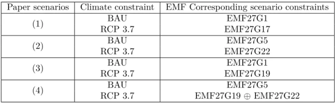
C

Matching between EMF27 and paper scenarios

Paper scenarios Climate constraint EMF Corresponding scenario constraints

(1) _{RCP 3.7}BAU _EMF27G17EMF27G1

(2) _{RCP 3.7}BAU _EMF27G22EMF27G5

(3) _{RCP 3.7}BAU _EMF27G19EMF27G1

D

Emissions trajectories

D.1

Emissions trajectories for EMF27 study

2000

5

2020

2040

2060

2080

2100

0

5

10

15

20

25

30

35

40

RCP 3.7 W/m2

RCP 2.6 W/m2

Figure 7: Emission trajectories (Gt CO2)

D.2

Emissions trajectories for additional discussion case

5 10 15 20 25 30 35 40 2010 2020 2030 2040 2050 2060 2070 2080 2090 2100

E

Imaclim-R model schematics

Public Administration

Redistribution & Infrastructures

Exports

Imports

World goods, services and capital markets

12 regions

12 sectors (5 energy, 3 transports, construction, industry, agriculture, composite)

(a) Static equilibrium

TR

ANSP

ORT

OI

L

SU

P

P

LY

IN

DU

ST

RY

E

LE

CTRICITY

E

N

E

RG

Y

E

FF

ICI

E

NCY

under updated constraints

(b) Model dynamics

F

Electricity demand

bau hghBio ccsOn bau hghBio ccsOf bau lowBio ccsOn bau lowBio ccsOf

550 hghBio ccsOn 550 hghBio ccsOf 550 lowBio ccsOn 550 lowBio ccsOf

G

Electricity mixes

2020 2040 2060 2080 2100 0 20 40 60 80 100 coalWoCcs coalWCcs gasWoCcs gasWCcs oil nuke hydro wind becc beccs solar unused (b) Low biomass potential and CCS available (2)

2020 2040 2060 2080 2100 0 20 40 60 80 100 coalWoCcs coalWCcs gasWoCcs gasWCcs oil nuke hydro wind becc beccs solar unused (c) High biomass potential and CCS unavailable (3)

2020 2040 2060 2080 2100 0 20 40 60 80 100 coalWoCcs coalWCcs gasWoCcs gasWCcs oil nuke hydro wind becc beccs solar unused (d) Low biomass potential and CCS unavailable (4) Figure 11: Global electricity mix under two biomass resource constraints (RCP 3.7 – no CCS)

H

Investments

bau hghBio ccsOn bau hghBio ccsOf bau lowBio ccsOn bau lowBio ccsOf

550 hghBio ccsOn 550 hghBio ccsOf 550 lowBio ccsOn 550 lowBio ccsOf

(a) Investment in the electricity sector

2020 2040 2060 2080 2100 0 200 400 600 800 1000 1200 1400 1600

bau hghBio ccsOn bau hghBio ccsOf bau lowBio ccsOn bau lowBio ccsOf

550 hghBio ccsOn 550 hghBio ccsOf 550 lowBio ccsOn 550 lowBio ccsOf

(b) Investment in the agricultural sector Figure 12: Additional investment needed