Application of life cycle costing method to a renovation project

Application of Life Cycle

to a Renovation

Costing

Project

Method

SUBMITTED TO THE DEPARTMENT OF ARCHITECTURE IN PARTIAL FULFILLMENT OF THE REQUIREMENTS FOR THE DEGREE OF

SCIENCE MASTER IN BUILDING TECHNOLOGY AT THE

MASSACHUSETTS INSTITUTE OF TECHNOLOGY

JUNE 1996

Copyright @ 1996 by Makoto TANEDA. All rights reserved. The author hereby grants to MIT permission to reproduce

and to distribute publicly paper and electronic copies of this thesis document in whole or in part.

Signature of Author:_

Department of Architecture May 10, 1996 Certified by:

Leonard J. MORSE-FORTIER Assistant Professor of Building Technology Deparfment of Architecture Accepted by: -AS1AcusE rTS LNSTE OF TECHNOLOGY

JUL 1 91996

g

THESIS READERS:

Leslie K. NORFORD

Associate Professor of Building Technology Department of Architecture

Robert D. LOGCHER

Application of Life Cycle Costing Method

to a Renovation Project

by

Makoto TANEDA

Submitted to the Department of Architecture

on May 10, 1996 in Partial Fulfillment of the

Requirements for the Degree of

Science Master in Building Technology

ABSTRACT

In this study, we have examined the application of LCC analysis method to the construction and renovation stages of a building project. The application of the LCC analysis is

currently limited to the very early stages of a project life, namely at the concept and design stages. We propose application of the LCC method, with several modifications, to the construction and renovation stages.

The simplified LCC method is proposed and examined in the first two case studies. The simplified method limits the range and complexity of data inputs, and is intended to be an LCC used by engineers practicing in the construction industry. In the third case study, the "LCC per square-foot", which implements the concept of the "square-foot" cost estimating, is proposed. This method is intended to be used to assess the residual value and to estimate running costs of an existing building. Necessary modifications of the LCC, as well as the accuracy and limits of these new methods are examined through three case studies.

Thesis Supervisor: Leonard J. MORSE-FORTIER Title: Assistant Professor of Building Technology

ACKNOWLEDGMENTS

The writing of this paper was made possible through a grant from Toda Corporation, and I would like to acknowledge their generosity. I wish to express my gratitude to Professor Ishifuku of Waseda University, most renowned LCC scholar in Japan, for providing me access to his research facility during the initial stage of this research. I also wish to

express my special gratitude to my family, Molly, John, Sarah and Akane, who have supported and encouraged me for two years.

Makoto Mike TANEDA

-TABLE OF CONTENTS

0.1 Abstract... 3 0 .2 T hesis ... 6 0.3 Introduction ...- 6 1. Attributes of LCC

1.1 Life Cycle Costing...7 1.2 O n F inance ... ... 1 1 1.3 Conclusions and Suggestions ... 1 6 2. Examination of Simplified Life Cycle Costing

2.1 Case Study No.1: LCC of Insulation Material...1 9 2.2 Energy Model Calculations ... 40 3. Application of Life Cycle Costing to Construction

3.1 Running Costs ... 46 3.2 Sensitivity Analysis ... 5 0 3.3 Case Study No.2: LCC of Curtain Wall System ... 5 1 3.4 Energy Model Calculations ... 7 6 4. Life Cycle Costing as a Value Assessment Tool

4.1 Concept of Residual Value ... 88 4.2 Case Study No.3: Retrofit LCC... 97 5. Conclusion... ... 11 4 6. Bibliography ... 11 5

THESIS

The LCC analysis method can be used to make decisions in the construction and renovation stages of a building project.

INTRODUCTION

Everyone seems to agree that LCC (Life Cycle Costing) is a good idea. Using the LCC analysis method, one can estimate the total cost of a project including its running cost in addition to its initial capital cost. The concept became especially well known after the energy crisis in 1974. Many scholars write as if the LCC analysis is the industry standard for making every major decision in a building project.

I have been in practice as a construction engineer and consultant in a Japanese construction firm for 8 years (1987 to 1994), never using the LCC analysis. When I came to know more about the benefits of this method, a question arose: Why is the LCC

analysis not conducted among construction engineers? This was the starting point of my study. The original intention was to understand and find a way to use this technique within my professional practice. However, as soon as it began, I faced many obstacles.

The first difficulty was my lack of understanding of many financial terms. These terms, which are not taught to engineers, make up the essential part of the LCC method. The next problem I encountered was the lack of a solidly established LCC method. Although various LCC studies agree in concepts, there are many inconsistencies in the procedure and formula. Probably the largest difficulty was the lack of available running-cost data. Even though there are so many running-cost guidebooks published annually, it is still extremely difficult to obtain desired data on running (maintenance and renovation) cost.

This study examines the possibility of applying the LCC method to the

construction, renovation and maintenance stages of a building project. Proposed solutions to overcome these existing obstacles are presented as examples in the case studies.

1. ATTRIBUTES OF LIFE CYCLE COSTING

1.1 Life Cycle Costing

Known since the 1960s as "Costs-in-Use" or "Total Building Cost Appraisal" (Brandon, Spedding, ed.,1987), Life Cycle Costing (LCC) analysis is defined by Ruegg (1980) as:

"A general method of economic evaluation which considers all relevant costs associated with an activity or project during its time horizon, comprising the techniques of total life-cycle cost, net savings, internal rate of return, and savings-to-investment or benefit/cost ratio analysis."

It will be necessary to briefly discuss the definition of LCC. In the course of this discussion, some of the reasons which limit the application of the LCC to the initial

conceptual and design stages will be depicted.

1.1.1

Components of the LCC

Various scholars basically agree that LCC is the sum of the initial cost and the operational costs over the life span of a building. According to Magee (1988) LCC includes:

- Initial costs - Iperating costs

- Indirect maintenance costs

- Direct maintenance costs

- housekeeping - general maintenance - preventive maintenance - repair - replacement - improvement - modification - utilities

Researchers of LCC, like Dell'Isola and Flanagan, slightly widen the definition. Dell'Isola (1983) describes the LCC as "all significant costs of ownership," the categories include:

. Initial costs - Financing costs

- Operation (energy) costs - Maintenance costs

- Alteration/replacement costs - Tax elements

- Associated costs - Salvage value

Flanagan (1989) states that LCC is the "total cost of a project" which includes: - Initial capital cost

. Running costs

- annual and intermittent maintenance

- cleaning

- energy

- security

- general and water rates

Clearly, it can be seen that there is no agreement among the scholars on the precise scope of LCC components. In this thesis, which examines new applications of LCC for the

construction industry, the categories are confined to: - Initial capital cost

- Running costs

- annual maintenance cost

- annual energy cost

- intermittent renovation cost

1.1.2

Percentage of LCC

The contribution of each of the above categories will vary significantly for each project and the length of the analysis. Shear (1983) emphasizes the importance of maintenance costs by a chart (reproduced here as Chart 1.1-1) which describes an LCC distribution for 50 years: Design % 3% Conception Construction 2 0 0%... Maintenance Copyright @ 1983 75% by M.A. Shear

Chart 1.1-1: Percentage of Life Cycle Costs

Maint. Other Maint. Annual _5% 7% 10% Energy.. Capital E nergy ... .. 42% 1.6% Rates Copy rig ht @ 1989 20% by R. Flanagan

Chart 1.1-2: LCC of an Office building

Though not exactly in the same context, Flanagan (1989) shows a lower percentage for the maintenance costs. Chart 1-1-2 is a reproduction from several examples of a 40 year LCC calculation. The total cost here is the capital cost and the running cost, with running costs making up 58% of the total.

Although the ratios are different, both examples show that the running costs dominate the total costs. The scale of impact of the cost segments and other parameters on total costs will be studied later, using the results from the case study (Section 3.3).

1.1.3

Control over LCC

There is a very persistent notion among the scholars of LCC that effective control over the LCC can be done only in the early stages of a project. For example, Magee (1988) states that:

"As soon as the life of the building or component begins, the control (or flexibility) of the total life cycle cost of the facility diminishes."

Dell'Isola (1975) states that the decision of the owner-using agency governs the total project expenditure. The scale of impact on total costs is described by a figure in his book (reproduced here as Figure 1.1-1).

Using agency's

,.A standards & cr

0 o.-Architect 0 E Copyright @ 1975 by A. Dell'lsola iteria - engineer Initial contractor

Operation & maintenance personnel

Time

Fiaure 1.1-1: Maior Decision Makers

Other scholars express similar notions on this point (Flanagan, 1983, Ruegg, 1980). Therefore, their books are often designer oriented. We agree that an LCC analysis at later

stages of building project life will not be able to have a profound impact on the total project cost. Still, this study attempts to apply the LCC method to the "down-stream" stages: construction, renovation and maintenance. Our reasoning will be explained later (Sections

1.2 On Finance

1.2.1 Time Value of Money

There are many financial terms that need to be understood to conduct the LCC analysis. As the Life Cycle Costing deals with various expenditures which occur at different points in time, the costs are all adjusted to their "Present Value" (PV) to maintain consistency. The process of adjustment becomes very complex when the analysis period extends over decades.

The basic principle is quite simple, being among the first topics learned in the study of finance. One hundred dollars today is worth more than $100 a year from today, because if it were invested for a year it would have generated an appropriate interest. Although we are dealing principally with costs and not with investments, the concept that the value of money changes over time is identical. The various documents on LCC, maintenance, real estate and finance utilize similar formulae to obtain the "Future Value" (FV) of a present

amount (PV) invested for "n" years at an annual interest rate of "i":

FV = PV(l + i)" (1)

where

FV = Future Value PV = Present Value

i= annual interest rate n = number of years

The present value can be obtained by manipulating formula (1) to the form: 1

PV = FV (2)

(1+i)"

1.2.2

Discount Rate

Unfortunately, the uniform accord among various documents seems to come to an end at this point. The definitions of "Discount Rate" or "Discounting Factor" differ in almost every source. In 'Real Estate Finance and Investment' (Brueggemen, 1993), the discount factor is defined as being the ratio of the present value over the future value. The discount factor, "d", in this case, would be:

1 PV=FV (1+i)" PV FV 1 d = 1(3) (1 + i)" d = discount factor

Flanagan (1989) simply treats the interest rate as the discount rate. The interest rate becomes the discount rate when trying to obtain the present value:

FV

PV = FV(4)

(1+ d) (

where

FV = Future Cost in year n

d = Discount rate n = number of years

In books on financial theory the terminology seems to be quite different. Hull (1993) refers to the discount rate as being "the annualized dollar return provided by an investment expressed as a percentage of the face value."

360 (FV -PV) (5)

n 100

where

d = discount rate

FV = Future Face Value of investment

PV = Present cash price

n = number of days to maturity

In this paper, as the LCC analysis principally assesses costs and not investment (Ruegg, 1980), the concept of the discount rate is based on formula (4).

1.2.3

Net Discount Rate

As stated earlier, the LCC analysis primarily deals with costs. The discount rate is utilized merely as one of the calculation factors which is applied to each option uniformly. There is no concern for the risk component in this case. However, as the options might have different inflation rates, it will be necessary to separate the inflation component from the discount rate. Flanagan defines this risk-and-inflation-free discount rate as the "Net Discount Rate":

dn= -1 (6) where

dn = net of inflation discount rate

i = interest rate including inflation

E = inflation rate

Therefore, the term "discount rate" in this paper means "net discount rate", according to formula (6).

If inflation is considered separately elsewhere, or is not considered at all, the net discount rate will be:

dn (1 +i) _I [(1+ E)l_(1+i)

_ 1

=(1

+i)-Only in these special situations, the net discount rate will exactly equal the interest rate, or:

Net Discount Rate = Interest Rate

The present value, adjusted for the influence of the inflation component is called "Net Present Value" (NPV). And it is defined as:

NPV= FV7) (1+ dn)"

where

NPV = Net Present Value

FV = Future Cost in year n

dn = net discount rate n = number of years

The most important point is to be consistent about the inflation and discount rates. (Ruegg, 1980) When costs include inflation, the net discount rate must be used. When costs do not include inflation, the discount rate must be used.

1.2.4

Present Value of Annual Cost

The advantage of formula (6) can be seen when dealing with annual costs. These costs will be influenced by the rate of inflation, as well as by the interest rate. The present value of cost "C" at year "t" can be expressed as:

C, =Cx(1+E)' PV = C x (1+ E)' (1+ i)' =Cx (1+E)

S(1+

C = Cost at year 0 (Present Estimate)

C₁ = Cost at year t

i = interest rate

E = inflation rate dn = Net discount rate

The simple formula (8) can be used to calculate the present value of costs with different inflation rates (i.e., labor and material). This formula (8) can further be incorporated with the formulae of Miles (1987) in order to obtain the total sum of the annual costs. "Present Value of the Cost Flow" (PVCF) will be:

"1 PVCF =Cx I ,= (1 + dn)'

Fl1

11

PVCF = Present Value of annual Cost Flow

n = number of years

In order to simplify the formula, both sides of the equation are multiplied by (1+dn) to produce:

(1+dn) X PVCF

1i 1 1 1__ _ _

=(C + + 2 +)... + (10)

11 (1+ dn) (1+ dn) (I1+ dn)"~

The right hand sides of the equations (9) and (10) are identical except for the last item in (9) and the first item in (10). So, by subtracting equation (9) from (10), the whole formula is simplified to:

dnxPVCF=Cx 1]- (11)

(1 + dn)"

By dividing both sides of the equation (11) by the net discount rate "dn", a relatively simple formula is reached:

1

-

1

IL

(1

+

dn)"

PVCF =C x - (12)

dn

In this paper, equation (12) is used to calculate the sum of the present value of annual costs.

1.2.5

Interest Rate

The interest rate in this paper is "compound interest rate" or compounded only once per annum. It will be appropriate to deal with flows of the costs which extend over a period of

15 to 75 years. The primary source of the interest rate is Table No. 820 from 'Statistical

Abstract of the United States 1995' (U.S. Department of Commerce, 1995). Past records

of the effective rate of Federal funds are used to estimate the interest rate to be used within the calculation. Also it should be noted that the interest rate obtained this way is assumed

to be a "risk-free" but "inflation-compounded" interest rate. The components of inflation are dealt with when converting the interest rate to the net discount rate.

"Internal rate of return" and "benefit/cost ratio" analyses will be explained and conducted in the first case study (Section 2.1).

1.3

Conclusions and Suggestions

1.3.1

Reasons for the Limited Application of LCC

The following are the possible reasons which obstruct a wider application of the LCC method.

1.3.1.1 Concepts

As mentioned in Section 1.1, there is a strong notion among scholars of LCC that analysis is most effectively conducted at the earliest stages of a project. Conceptual and design stages for new construction, which have the largest control over the building LCC, are defined as the only applicable segments.

1.3.1.2 Complexity

Proponents of LCC describe the method as simple. However, as can be seen from sections 1.1 and 1.2, it is far more complicated than ordinary estimating of initial capital costs. Many terms are unfamiliar to persons normally engaged in construction and maintenance. The operations involved in LCC are more complex than the ordinary multiplication and addition of construction cost estimates.

1.3.1.3 Data

The maintenance costs and the life expectancy of building components are difficult to assess compared to the initial construction costs which are easily obtainable from widely accepted estimation handbooks.

1.3.2

Objections and Solutions

1.3.2.1 Concepts

All stages in a building's life have some control over the costs which occur in the future. Also, unless the LCC design and concept are properly understood and executed by persons in later stages, a project's actual costs will differ from its expected life cycle performance. There seems to be no reason to limit the application of LCC to the conceptual and design stages.

It is suspected that the limited application originates from LCC's complexities. The execution of the complex LCC analysis requires high costs which needs to be justified from a large project expenditure saving. The early stages are the only time this large saving is

possible. However, if a simplified and less costly LCC analysis is possible, downstream decisions may be better informed even where potential savings are reduced.

1.3.2.2 Complexity

The financial and LCC terms are eventually understandable. Their meanings and relations can be expressed mathematically, allowing engineers to understand them. Sections 1.1 and

1.2 represent examples of how to reason through various contradictory definitions. In our case, the single difficult point was the determination of the financial rates: interest,

discount and inflation rates. Various studies about LCC do not describe thoroughly how to obtain the appropriate information to set these rates.

The complexity of calculations can be overcome easily with a personal computer and a spreadsheet program. Recent major spreadsheet programs have various useful functions that can help LCC calculations. (i.e., Lotus 123, Microsoft Excel)

1.3.2.3 Data

Collected LCC data will be a powerful tool to conduct the analysis and will save substantial research time. However, there are very few documents that actually collect LCC data

(Dell'Isola, 1983 and NBA Construction Consultants, 1985). It is possible that the scarcity of LCC data originates from the limit of the LCC application. There are many differences, in accounting style and labor segments, as well as between the construction and maintenance industries. Unless given proper incentive to provide useful information, feedback from the maintenance industry will lack the necessary qualitative characteristics to support LCC (Ashworth, Spedding ed., 1987). Also, it is unrealistic to expect information feedback from people who do not correctly understand its purpose.

A short term solution, used in this thesis, is to substitute data from other sources for use in the LCC . Where possible, we have limited the data inputs to the ones easily available and widely accepted.

The long term solution would be to develop a better and wider understanding of the LCC concept across the construction and maintenance industries. The ideal results would

be constant feedback of maintenance data, for example, in the form of the annual (or regular) publication of LCC data from major construction cost handbook publishers.

1.3.3

Scope of the Case Studies

1.3.3.1 Examination of Simplified LCC

The first case study examines the accuracy of a simplified LCC. The primary purpose of the analysis is to provide an LCC comparison of choices for a building component.

Basically, the analysis format follows Flanagan (1989) with the data inputs made as simple as possible. The scale of the data simplification is assessed by comparing the LCC and other analyses results.

1.3.3.2 Application of LCC to Construction

The second case study examines the application of the LCC method to the construction stage. The subjects of LCC analysis is a large building system. Using the findings from the first case study and from an appraisal of the running costs, a format for the simplified and reasonable LCC analysis is presented. Furthermore, a sensitivity analysis is conducted to assess the importance of various LCC parameters.

1.3.3.3 LCC as a Value Assessment Tool

The third case study proposes the use of the LCC method as a tool for evaluating the value of an existing building. A new format using the concept of "cost per square-foot" is presented.

2.

EXAMINATION OF SIMPLIFIED LIFE

CYCLE COSTING

2.1 Case Study No.1:

Life Cycle Cost Analysis of

Insulation Material

2.1.1

Scope of the Case Study

The scope of this study is to apply the Life Cycle Costing (LCC) analysis method on a small scale range. The LCC analysis is widely recognized to be potentially superior to the initial capital cost comparison. However, the method is usually used to compare choices for large-scale systems like HVAC. Complex handling of numbers and the laborious collection of necessary data are obstacles to its use on an everyday level.

This case study is intended to demonstrate that using the basic cost data normally available to the practicing engineer and with the help of a spread-sheet program on a personal computer, it is possible to conduct an accurate LCC analysis, even for a small decision point. To test its accuracy, comparisons with other common appraisal techniques

are also conducted. An attempt to employ a more advanced LCC method forms the subject of the next study, using the feedback from this study.

2.1.2

Selection of the Analysis Subject

2.1.2.1

Selection

The LCC method is most appropriate when evaluating subjects which combine operating costs with capital investment. However, there is no common standard for estimating running costs within the building industry. The condition of use which has a direct impact on maintenance varies considerably among buildings and at different locations. Dell'Isola (1983) is one of the few authors who has attempted to present a standard for maintenance cost, but the number of entries in his handbook is very limited compared to the available capital cost data.

In this case, we have selected insulation materials as the subject of LCC analysis. To substitute the running cost, we use the annual energy cost saved by using each material,

calculated according to a standardized method, and is converted to an objective and justifiable cost flow.

2.1.2.2 Characteristics of Insulation Basic Materials

According to the American Society of Heating, Refrigerating and Air-Conditioning Engineers (ASHRAE, 1993), thermal insulations normally consist of the following basic materials:

. Inorganic, fibrous, or cellular materials such as glass, rock, or slag wool; calcium silicate, bonded perlite, vermiculite; and asbestos.

- Organic fibrous materials such as cotton, animal hair, wood, pulp, cane, or synthetic fibers, and organic cellular materials such as cork, foamed rubber, polystyrene, polyurethane, and other polymers.

Types and Classification in this Study

In this study, we divide the insulation materials into three groups according to their finished products, though basically following the division by ASHRAE. From each group, rigid and non-rigid products with thermal resistance value (R-value) around 10 are chosen, when possible, as the options for analysis.

Group I: Silicate Based Beads

Silicate based materials are usually produced in the shape of small beads. They are physically and chemically very stable, not affected by temperature below 1000'F, and they are virtually unchanging through time. This group includes:

- Perlite

. Vermiculite

. Insulating Concrete

Group II: Mineral Wool Batt and Board

These are glassy fibrous substances made by melting and fiberizing minerals. These are stable materials because of their inorganic nature, but fine fibers melt at a temperature above 200'F.

. Mineral Fiber Batt

Group III: Cellular Insulation Board

Cellular insulations work by using the thermal resistance of air or other gas

contained in the cells. Some are made of organic materials like paper or wood, but polymer plastic based products are common in the current construction industry.

Those which use thermally high resistant gas instead of air may suffer slight performance degradation due to the diffusion of their cell contents.

. Expanded and Extruded polystyrene Board Polyurethane and Isocyanurate Board - Urea-Formaldehyde and Urea-Based Foam

2.1.3 Methods of Analysis 2.1.3.1 Methods of Analysis

We have conducted three types of analysis, including the LCC. Unit Cost Analysis

The initial costs of the options are compared with the same applied unit. This is the simplest cost comparison and is universally conducted.

Financial Analysis

Costs and savings of the options are compared using the financial appraisal techniques. "Benefit-cost ratio" and "Rate of return" are calculated.

- Benefit-cost ratio is, in our case, the ratio of savings to the initial investment. . The rate of return is defined as "the discount rate that gives a net present value

of zero." (Couper, 1986) It yields the rates to compare from which one can compare the speed of investment recovery.

LCC Analysis

The LCC method compares the sum of the initial investment and running costs over the estimated life of the subject. The costs, which occur at different points in time, are adjusted to the same standard of the Present Value (PV). The discount rate necessary to obtain the PV is defined by the inflation and the interest rates.

2.1.3.2 Common Data Input Economic Data

Capital Cost and Inflation Rate

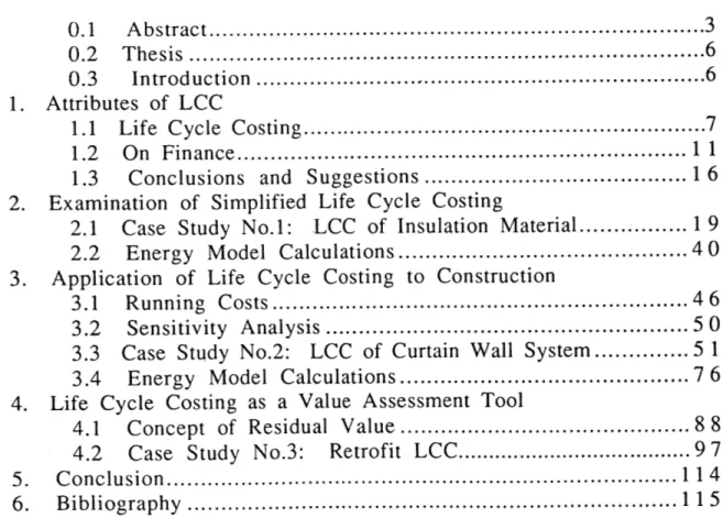
Capital costs are obtained from the cost data handbooks that are widely accepted within the construction and architecture industry. They are renewed annually to provide accuracy which also enables us to calculate the rate of change. The cost of each insulation material is from 'Means Building Construction Cost Data' (1995). The estimated cost data for the year 1996 is used as the material cost (Table 2.1-1). The inflation rates are calculated from the last 6 years' costs (Table 2.1-2).

Abbreviations used within the tables include:

- 1 Carp: Requires I carpenter to install

- CF: Cubic Foot

- SF: Square Foot

- O&P: Overhead and Profit

Tables 2.1-1 and 2.1-2 are presented in the format of Means handbook. The summary of those material costs and inflation rates which suit our purpose comprise Table 2.1-3.

.... ...... .... ....~L

110 .0010 POURED INSULATION

.0020 Cellulose, R3.8/inch 1Car 200 .040 CF .41 1.01 1.42 2.06

.0040 Perlite, R3.2/inch , , 200 .040 ,, 1.50 1.01 2.51 3.26

.0080 Fiberglass wool, R4/in. ,, 200 .040 ,, .31 1.01 1.32 1.95

.0100 Mineral wool, R3/inch 200 .040 .32 1.01 1.33 1.96

.0300 Polystyrene, R4/inch ,, 200 .040 ,, 1.72 1.01 2.73 3.50

.0400 Vermiculite, R2.7/inch ,, 200 .040 ,, 1.50 1.01 2.51 3.26

.0700 Wood fiber, R3.85/inch ,, 200 .040 ,, .56 1.01 1.57 2.23

116 .0010 WALL INSULATION, RIGID Fiberglass, 3#/CF, -. 0300 unfaced .0370 1" thick, R4.3 1Car 1000 .008 SF .32 .20 .52 .67 -. 0420 2-1/2" thick, R10.9 , , 800 .010 , , .88 .25 __1.13 1.37 Isocyanurate, 4'*8'

.1600 sheet, foil faced

.1610 1/2" thick, R3.9 1Car 800 .010 SF .27 .25 .52 .70 .1650 1-1/2" thick, R10.8 ,, 730 .011 ,, .67 .28 .95 1.18 .1700 Perlite -.1710 1" thick, R2.77 1Car 800 .010 SF .31 .25 .56 .74 Extruded polystyrene, .1900 25 PSI compressive .1920 1" thick, R5 1Car 800 .010 SF .31 .25 .56 .74 .1940 2" thick, R10 ,, 730 .011 ,, .57 .28 .85 1.07 .2100 Expanded polystyrene .2110 1" thick, R3.85 1 Car 800 .010 SF .18 .25 .43 .60 .2140 3" thick R11.49 ,, 730 .011 ,, .54 .28 .82 1.03 118 .0010 WALL OR CEILING INSUL, NON-RIGID

Fiberglass, kraft faced,

.0040 batts or blankets

.0080 d=3.5", R11, w=15" 1Car 1600 .005 SF .20 .13 .33 .42 Mineral fiber batts,

.1300 kraft faced

.1320 3.5" thick, R13 1Car 1600 .005 SF .32 .13 .45 .55 Copyright C 1995 by R.S. Means Co., Inc.

Insulation Costs for Year 1996

Table

1 101 .0010 POURED INSULATION

.0020 Cellulose, R3.8/inch 3.8 -3.4% 2.7% 0.7% 1.8%

.0040 Perlite, R3.2/inch 3.2 -4.5% 2.7% -1.6% -0.6%

0080 Fiberglass wool, R4/in. 4.0 -2.8% 2.7% 1.3% 2.3%

.0100 Mineral wool R3/inch 3.0 -20.9% 2.7% -6.3% -4.0%

.0300 Polystyrene, R4/inch 4.0 0.4% 2.7% 1.2% 1.8%

.0400 Vermiculite, R2.7/inch 2.7 -4.5% 2.7% -1.8% -0.8%

.0700 Wood fiber, R3.85/inch 3.9. 1.0% 2.7% 2.1% 2.8%

116 .0010 WALL INSULATION, RIGID Fiberglass, 3#/CF, .0300 unfaced .0370 1" thick, R4.3 4.3 1.0 -4.8% 2.4% -2.4% -1.4% .0420 2-1/2" thick, R10.9 10.9 2.5 -4.9% 2.7% -3.4% -2.8% sheet, foil faced, both

.1 6001sides .1610 1/2" thick, R3.9 3.9 0.5 1.0% 2.3% 1.6% 1.9% .1650 1-1/2" thick, R10.8 10.8 1.5 -3.2% 2.7% -1.6% -0.9% .1700 Perlite 1710 1" thick, R2.77 2.81 1.0 -6.3% 2.7% -2.8% -1.9% 25 PSI compressive 1.1900 strength .1920 1" thick, R .0 1.0 -6.1% 2.7% -2.7% -1.7% H .1920 " thick, R 10 1.0 .0 - . % 2.7% -2.7% -1. % .2100 Expanded polystyrene I .2110 1" thick, R3.85 3.9 1.0 0.1% 2.7% 1.6% 2.5% .2140 3" thick, R1R1.49 11.5 3.0 17.7% 3.8% 12.3% 10.7% 118 .0010 WALL OR CEILING INSUL, NON-RIGID

Fiberglass, kraft faced,

.0040 batts or blankets

.0080 d=3.5",' R11, w=15" 11.0 3.51 -5.8% 3.2% -2.8% -1.6%

Mineral fiber batts,

1.1300 kraft faced

I .1320 1d=3.5", R13 13.0 3.5 1.9% 3.2% 2.3% 2.4%

Inflation Rate Calculated from Means Data

I Perlite board 2" thick, R5.5 SF 1.48 -1.9%

|I Fiberglass board 2-1/2" thick, R10.9 SF 1.37 -2.8%

Fiberglass batt 3-1/2" thick, R11 SF 0.42 -1.6%

Mineral fiber batt 3-1/2" thick, R13 SF 0.55 2.4%

III Isocyanurate 1-1/2" thick, R10.8 SF 1.18 -0.9%

Extruded polystyrene 2" thick, R10 SF 1.07 -5.4% Expanded polystyrene 3" thick, R1 1.49 SF 1.03 10.7%

Running Cost

The insulation material itself does not require any maintenance. It is usually embedded within wall or roof system components, and replaced only when renovation of surrounding system necessitates it. In this paper we have used the

energy saving as the annually recurring cost. Interest Rate and CPI

The interest rate and the Consumer Price Index (CPI) figures are from the Statistical Abstract of the United States 1995. The interest rate for the calculation is set at 4.21%, from the effective rate of the Federal funds from 1994. CPI of Energy from 1985 to 1994 is used to estimate the inflation of the energy cost. These data are summarized in Table 2.1-4.

Table 2 1-4: Inflation Rate of Enerav

Consumer Price Indexes (CPI-U):

1984 103.9 100.9 1985 107.6 101.6 1986 109.6 88.2 1987 113.6 88.6 1988 118.3 89.3 1989 124.0 94.3 1990 130.7 102.1 1991 136.2 102.5 1992 140.3 103.0 1993 144.5 104.2 1994 148.2 104.6 fl R 3.9%1 1.1% Inflation Rate Table 2.1-3: Cost and

Energy Price

Average end-users' fuel prices of $0.60 per gallon of No. 2 fuel oil and 8.34 cents per kWh of electricity are used. (U.S. Department of Commerce, 1995)

Energy Data

ASHRAE Handbook of Fundamentals

In order to calculate annual energy consumption, an energy model was set up, based on an example from 'ASHRAE Handbook'. The model building (Figure 2.1-1) is a single story detached house, located in Chicago, with medium grade wood construction. 74' 24 100 20'24' -MASTER BEDROOM BATH BEDROOM 2 BEDROOM1 LIVING ROOM 8 ft. CEILING THROUGHOUT KITCHEN AND DINETTE GARAGE I .A STORAGE UTILITY AND SHOP - - - U

-All dimensions in feet

N

Fiaure 2.1-1: Plan of the Model

The worksheet of the energy cost calculation is supplied as the Appendix at the end of this chapter. The summary is given in Table 2.1-5.

24'

CLOSET

BATH

3

6'

.. .. .. . - . ....

_______________... _ _ _ _

I__

8__

iB u

Model no insulation 33,299 163,368

ASHRAE; wall R13, roof R191 1.55/.72 13/19 20,578 106,632

Perlite 2.00 1.07 5.55 25,331 125,283

|| Fiberglass, 3# 2.50 1.37 10.90 22,374 112,746 Fiberglass batts 3.50 0.42 11.00 22,339 112,585

Mineral fiber batts 3.50 0.55 13.00 21,635 109,718

Ill Isocyanurate 1.50 1.18 10.80 22,421 112,908

Extruded polystyrene 2.00 1.07 10.00 22,744 114,279 Expanded polystyrene 3.00 1.03 11.49 22,148 111,824

Energy Costs

Cooling costs are calculated assuming the use of a heat pump and an electric chiller. Using the efficiency factor, annual cooling energy requirement, Qc, is converted to energy consumption, Ec. Cooling cost is obtained applying already specified fuel price.

Ec =

Qc

Qc

Ec = Cooling energy consumption (kWh) P(elec) = Price of electricity ($ / kWh)

= 0.0834 ($ / kWh) Cc = Cooling cost ($)

Heating costs-are calculated assuming the use of an oil fuel boiler. Once annual heating energy requirement, Qh, is computed, corresponding energy consumption, Eh, is calculated from the system efficiency. Fuel consumption, F, and heating cost, Ch, are obtained applying consumption rate and price.

Eh F Ch = Qh / 0.65 = Eh I 14 4 0 0 0 = F x P(oil)

Qh = Heating energy requirement (kBtu) Eh = Heating energy consumption (kBtu)

F = Fuel consumption (gallon)

P(oil) = Price of oil ($ / gallon)

= 0.60 ($ / gallon)

Ch = Heating Cost ($)

The initial and annual energy costs of each model are given in

Table 2.1-6: Initial and Annual Energy Costs

Model no insulation 0 1,373

*ASHRAE; wall R13, roof R19 2,175 885

1 Perlite 3,564 1,051

II Fiberglass, 3# 4,563 941

Fiberglass batts 1,399 940

_ Mineral fiber batts 1,832 915

Ill Isocyanurate 3,931 943

Extruded polystyrene 3,564 955

Expanded polystyrene 3,431 933

Table 2.1-6.

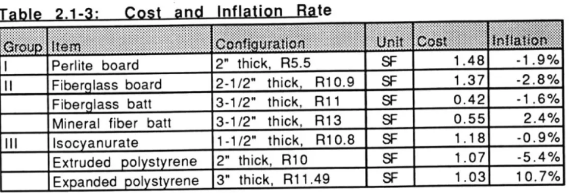
Degradation of Material

The thermal conductance, k, of expanded polystyrene degrades in the first 5 years from k=0.16 to 0.20. (Strother, 1990)

In attempting to take this degradation into account, the energy cost was calculated using each k-value. Assumption that the degradation continues at a constant rate will lead to an annual cost increase of 0.7%. However, another assumption with fixed k-value after reaching 0.20 will lead to an absolute cost increase of 3.7%. These are shown in Table 2.1-7.

Table 2.1-7: Energy Cost Change of Expanded Polystyrene

Y e~~ t~~c... .~n~ ...A b il~

0 2.00 0.16 12.50 21,794 110,379 921

5 2.00 0.20 10.00 22,744 114,279 955 0.7% 3.7%

2.1.4

Analysis Results

Insulation materials serve as the thermal barrier within the envelope of the building. In order to maximize the inner space of the building, thinner wall constructions are usually preferred. Therefore materials with larger R-values over small thickness are assumed to have better performance. To account for this fact, Means handbook supplies information

about R-value (energy performance) and thickness along with the simple unit cost of insulation materials. Using these data, we compare the subjects by their thermal resistance per thickness, their costs of per thickness and per unit of thermal resistance.

. Thermal resistance per thickness (R-value/inch): It indicates the energy performance obtainable per unit thickness. The higher it is the better the value.

- Cost per thickness ($/inch): Simple cost index.

. Cost per thermal resistance ($/R-value): It indicates the cost that the users pay per unit of energy performance. The lower it is the better the value.

The result is given in Table 2.1-8 with data of the poured insulation materials (beads form) as Group X for comparison.

Unit Cost of insulation Materials

Cellulose fiber, R3.8/inch 2.061 12.001 45.60 3.80 0.17 0.05

Perlite, R3.2/inch ,, 3.26 12.00 38.40 3.20 0.27 0.08

Fiberglass wool, R4/inch 1.95 12.00 48.00 4.00 0.16 0.04

Mineral wool, R3/inch ,, 1.96 12.00 36.00 3.00 0.16 0.05

Polystyrene, R4/inch ,, 3.50 12.00 48.00 4.00 0.29 0.07

Vermiculite, R2.7/inch ,, 3.26 12.00 32.40 2.70 0.27 0.10

Wood fiber, R3.85/inch ,, 2.23 12.00 46.20 3.85 0.19 0.05

1 Perlite SF 1.48 2.00 5.55 2.78 0.74 0.27

|1 Fiberglass, 3#/CF, unfaced 1.37 2.50 10.90 4.36 0.55 0.13

Fiberglass, kraft faced, batts ,, .42 3.50 11.00 3.14 0.12 0.04 Mineral fiber batts, kraft faced ,, .55 3.50 13.00 3.71 0.16 0.04

Ill Isocyanurate, 4'*8' sheet ,, 1.18 1.50 10.80 7.20 0.79 0.11

Extruded polystyrene ,, 1.07 2.00 10.00 5.00 0.54 0.11

I Expanded Polystyrene ,, 1.03 3.00 11.49 3.83 0.34 0.09

@ @

Copyright @ 1995 by R.S. Means Co., Inc.

@ @ @

R-value per thickness data are summarized in Chart 2.1-1. It can be seen that the rigid-board products (Group III and Fiberglass rigid-board) have the best energy performance relative to its thickness.

Chart 2.1-1: R-value ~er inch thickness

10.00 9.00 8.00 0 7.00 6.00 : 5.00 ' 4.00 3.00 2.00 1.00 .00 CO 0 4 _0 Table 2.1-8: thickness

The cost per thickness is summarized in Chart 2.1-2. This time, the Batt products of Group II are the best options.

Chart 2.1-2: Cost per inch thickness

The cost per thermal resistance is summarized in Chart 2.1-3. The Batt products of Group II are the best options, followed by the rigid-boards. Perlite in Group I has the worst result.

Chart 2.1-3: Cost ~er R-value

1.00 0.90 0.80 0.70 0.60 c 0.50 4 0.40 0.30 0.20 0.10 0.00 0 . 0 4 -2 co 0) 0) M J) Cd .0 C co 6 M-oC a. _{CU ) x} U_ U_ >% wU LI 0. 0.30 0.25 0.20 > 0.15 0.10 0.05 0.00 4) -o -_ c CUL~~4 1~ 0 as- x U_ U LU UD

2.1.4.2 Financial Analysis

In this section, initial and annual savings are compared instead of costs. Saving is

calculated by subtracting the cost of the baseline case from the corresponding costs of each option. The energy model with no insulation is used as the baseline case.

The initial and annual costs of the baseline case are $0 and $1,373 respectively. For example, an option using isocyanurate (Group III) has an initial cost of $3,931, so the

saving in initial stage will be a negative number of $-3,931. The same option has the annual energy cost of $943 which makes the annual savings $430. Initial and annual savings for each material are given in Table 2.1-9.

Table 2.1-9: Initial and Annual Savings

Model no insulation 0 0

ASHRAE; wall R13, roof R19 -2,175 488

__Perlite -3,564 322

|| Fiberglass, 3# -4,563 431

Fiberglass batts -1,399 433

Mineral fiber batts -1,832 458

IlIl Isocyanurate -3,931 430

Extruded polystyrene -3,564 418

Expanded polystyrene -3,431 439

Using financial terms, the initial cost of insulation corresponds to the investment. The annual energy cost of the uninsulated model is subtracted from energy cost of other options to yield annual saving or profit.

The present values (PV) of saving for the first three years are calculated with an interest rate of 4.21%. The ratio between the PV of saving and initial investment is the benefit cost ratio. The speed of return of the initial investment is the rate of return. These figures are presented-in Table 2.1-10.

Table 2.-10: Finncial.An...Re.i.it

.. ...

- .. ... _ ~ *~~~1~

Model no insulation 0 0 0

ASHRAE; wall R13, roof R19 -2,175 488 5,347 2.46 21%

1 Perlite -3,564 322 3,528 0.99 4%

11 Fiberglass board -4,563 431 4,726 1.04 5%

Fiberglass batts -1,399 433 4,741 3.39 30%

Mineral fiber batts -1,832 458 5,017 2.74 24%

Ill lsocyanurate -3,931 430 4,709 1.20 7%

Extruded PS -3,564 418 4,578 1.28 8%

Expanded PS -3,431 439 4,814 1.40 10%

The benefit-cost ratio is summarized in Chart 2.1-4. The Batt products in Group II the best ratio, followed by rigid-boards of Group III. Perlite in Group I shows the result.

Chart 2.1-4: Benefit-Cost

have worst

Ratio

The rate of return is summarized in Chart 2.1-5. The chart shows a close resemblance to Chart 2.1-4, in shape and proportion. Again the options with Batt products are the best options. Other subjects also show identical ranking.

3.50 3.00 2.50 . 2.00 ". 1.50 1.00 0.50 0.00 0) o 10 _0 0 CU W 4-co/ 0) 0 .a. (0 aU . LI..a-ct X LL >% LU U

Financial Analysis Results

Table

Chart 2.1-5: Rate of Return

2.1.4.3 Life Cycle Costing

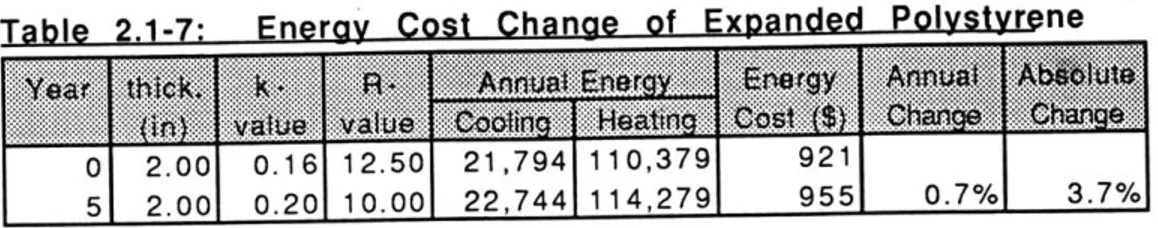
LCC analysis is conducted for each of the subject material choices. The format for the analysis is given as Table 2.1-11 which compares the LCC between each group. The cost profile for the same analysis is given as the Chart 2.1-6. As LCC is dealing with cost, the lesser is the better. Analysis is conducted for the period of 45 years with life expectancy of the material at 30 years. The interest and inflation rates are set at the figures described in Section 2.1.3.2.

Costs are divided into capital costs, annual energy costs and replacement costs. The capital costs are not discounted because they occur at year 0. The annual energy costs are discounted using the PVCF (Present Value of Cash Flow) factor. The replacement costs which occur at the end of the material life expectancy, are discounted using the PV discount factor. It should be noted that an individual inflation rate is applied to each material and further, that expanded polystyrene is presumed to have an annual degradation rate of 0.07%. 35% 30% S25% 20% 15% 10% 5% 0% 0 -2 Vo0 7 -0 CU M :3 =3i

L;- -0~0U 0 ~ L-a CU0a

Q- 0 0Cc

LL. C%$ w w

Table for LCC Analvsis Project Life Interest Rate (yrs)

( %)

dMi.sme

MW

PV~Ffae~X

Est. Est.

PV

3564 3564 4563 4563 3431 3431 178 228 172 3742 4791 3603 3.1% 3.1% 2.4% 24.19 24.19 27.54 1051 25427 941 22766 933 25697 25427 22766 25697 (year) (Disc. factor) 0 0.000 3564 0 31 0.154 3564 548 0 0.000 3564 0 0 0.000 3564 0 0 0.000 4563 0 31 0.115 4563 527 0 0.000 4563 0 0 0.0 4563 0 0 0.000 3431 0 31 6.507 3431 22326 0 0.000 ... 3431 33 0 0 0.000 3431 0 548 527 22326 TotaiNosts 29717 28084 51625 Table 2.1-11:

The profile of LCC can be seen in Chart 2.1-6. At year 31, though expanded polystyrene displays a large jump for replacement cost, other materials make only a small one. This is due to the difference in inflation rates projected for these materials.

The costs of the LCC analysis are given in Table 2.1-12. From the table and accompanying Chart 2.1-7, the result of the LCC analysis can be recognized. Once again, the Batt products in Group II are the best options. Other rankings are identical to other analysis methods, except that the expanded polystyrene, dropping from other options in Group HI, ends up to be the worst option.

o e 0 L Ya0

Year

Chart 2.1-6:

0 LA 0 LA

C~) '~-

'~-LCC Profile for Table 2.1-11

Table 2.1-12: Summary of LCC analysis

Perlite 29.717

11 Fiberglass board 28,084

Fiberglass batts 24,447 Mineral fiber batts 25,124

lil Iso-cyanurate 27,769 Extruded polystyrene 27,024 Expanded polystyrene 51,625 60000 50000 40000 30000 20000 10000 0 (1) Perlite - -- (II) FG Board (ll) Expanded PS Chart 2.1-6:

Chart 2.1-7: Chart for Table 2.1-12

2.1.5 Problems and Expected Solutions 2.1.4.1 Potency of LCC Method

Value

LCC brings the concept of time inghOe analysis. The results from each analysis have shown a close resemblance in ranking and proportion (Chart 2.1-3, 4, 5 and 7). Howeverthe LCC method is the only one which can display the points in time where a large increase of cost occurs or where one option becomes more favorable (or unfavorable) than another. Limit

Validity of Data

Analyses with multiple variable factors are influenced by the degrees of their validity. In our case the different inflation rates for each material had a predictable impacts on the analysis.

Consideration of Whole System

Batt products from Group II (Fiberglass and Mineral Batt) ended favorably in all of the analyses. Still, other products are also frequently chosen and used in actual construction. This seems to suggest that our analysis lacks certain considerations.

60,000 50,000 CA o 40,000 e 30,000 O 20,000 1 0,000 0 ((D .8 a. cola. 0- 0O 4-X LL LL w W w 0.

The LCC method, which takes into account the concept of time and use, needs to consider the relation of the subject element or system to the whole building. 2.1.4.2 Factors which need Further Consideration

Inflation Rate

In order to simplify the LCC method, we have used cost data from 1991 to 1996 (Means) to calculate the inflation rate of insulation materials. It turned out that these inflation rates varied significantly from minus 5% to plus 10%. These figures have a substantial impact

on future renovation costs in our calculation. However, as these materials are competing in the same small segment of the market, it is highly unlikely that their inflation rates continue to vary for the long term. Also, a negative inflation rate is not viable as a long lasting trend.

The range of data seems to have been insufficient for estimating the inflation trend of the next 45 years. Therefore it will be necessary to use (a) CPI as the inflation rates or (b) use a wider range of historical cost data. Option (a) will be easier to achieve but all materials will have the same inflation rate. Option (b) will have a more accurate inflation rate but requires significant time and difficulty in collecting sufficient information. Therefore, option (a) appears to be the practical choice.

System

Batt products from Group II ended favorably in all analyses. However, those "non-rigid" insulation materials have certain drawbacks when seen in the application level.

One drawback is in actual energy performance. As these materials need to be inserted within the supporting wall, the formed thermal barriers are usually obstructed at regular interval by the structural elements of the wall. As these elements may have very poor R-values, the actual R-value of the wall system becomes significantly lower than the calculated value.

Another disadvantage lies in their physical properties, which prevent them from becoming the base of further finish. Rigid boards, which can be the basis for finishes like

stucco or waterproofing, will be often chosen, and may reduce the costs of the enclosure overall.

These indicate that the simplified LCC analysis, as well as all other analyses in this section, lack the consideration of the actual constructed condition of the material. As the interaction among the material is an important factor in construction, even the simplified version of LCC should take it into account. Therefore it will be more practical to start the analysis from the system level.

Thickness

Another factor which could not be included in the analysis, though related to the problem of the system, is the thickness of each material. The thickness of the building envelope is often restricted by the building code which regulates the maximum building size and the owner who wants maximum rentable or lettable space. In an extreme case, the thickness of

the wall can be converted to the amount of annual rent income from its occupying space. For example, if the R-value of two materials is identical, it will be necessary to compare the cost and the thickness in terms of the LCC income.

2.1.4.3 Revised LCC Result

Before going to the next case study, the result of a partially revised LCC is presented here. - The inflation rate is set at 3.9% per annum from change rate of Consumer Price Index of years 1984 to 1994. In this revised analysis ,the same rate is applied to all options.

- The degradation factor of expanded polystyrene is changed from the annual rate of 0.7% to the absolute percentage of 3.7%. This is due to the perception that

continuous degradation of performance is unlikely.

- The results are given in Table 2.1-13 and Chart 2.1-8. The Batt products remain the best options as they did in the earlier result. However, the expanded polystyrene is now in the next ranking group with other rigid-board products in Group III.

_ _ Perlite 32,419

I Fiberglass board 31,717

Fiberglass batts 25,486

Mineral fiber batts 25,730

III Iso-cyanurate 30,526

Extruded PS 30,096

Expanded PS 30,138

Chart 21-8: Chart for Table 2.1-13

35,000 3 30,000 c 25,000 0 20,000 15,000 C.) 10,000 3 5,000 0 o o *_*0 co -:3 C/ ci~ ~ cC/)

SL

Revised Life Cycle Cost

Table

2.1-13:

2.2 Appendix to Case Study No. 1:

Calculations

Energv Consumption of a Sinale-familv Detached

Adaptation from "ASHRAE Handbook of Fundamentals 1993" Chapter 25 Residential Cooling and Heating Load Calculations Example 1 page 25.5

CONDITIONS

Geography

Geometry

Location Chicago, Illinois

latitude 41.8 (*N) cooling DD (650F) 713 (*F day) heating DD (650F) 6127 (*F day) E/W wall 74 f t N/W wall 3 6 (ft) ceilinq 8 (f ) Area 2664 (sqft) Volume 21312 (cft) Roof constru Wall constru ction

outside air film 0.25 0.17

gypsum roof deck 9.00 9.00

fibrous batt insul. 19.00 19.00

vapor retardant 0.12 0.12

inside air film 0.76 0.61

total 29.13 0.03 28.90 0.03

ction

outside air film 0.25 0.17

face brick 1.00 _ 1.00

fibrous batt insul. 13.00 13.00

polystyrene sheath. 1.88 1.88

gypsum board 0.45 0.45

inside air film 0.68 0.68

total 17.26 0.06 17.18 0.06

Floor construction

4-in concrete slab on ground

Energy Model

Fenestration

Clear double glass, 0.125 in thick

Assume closed, medium color venetian blinds The window glass has a 2 ft overhang

Assume outdoor storm sash, 1 in air space Doors

ni0.25

outside air film 0.25 0.17

all-glass storm door 0.50 0.50

solid core flush 1.70 1.70

inside air film 0.68 0.68

total 3.13 0.32 3.05 0.33 Design conditions outdoor dry-bulb 91 2 *0 F) d.range 15 *0_F) wet-bulb 77 *0_F)

indoor

dry-bulb

75

70

*0

F)

appliance kitchen 1600 (Btu/h)

utility 1600 (Btu/h)

construction average grade (N/A)

COUNG LOAD

Basic formula are: Walls, roof and doors

q= UA*(CLTD)

Windows

q= A*(GLF)

Air Change Rate:

ACH= 0.48

Cooling loads for the living room: Infiltration Q= ACH*(room volume)/60 = ACH*(3840)/60 = 31 q= 1.1*Q*(outside T-inside T) = 541 (Btu/h) Occupants q= 230*(persons) = 920 (Btu/h)

Appliances C Cooling loa

Infiltration

= 50%*(kitchen appliance load)

= 800 (Btu/h)

ds for the kitchen:

Q= ACH*(room volume)/60 = ACH*(1920)/60 = 15 q= 1.1*Q*(outside T-inside T) = 270 (Btu/h) Appliances q= 50%*(kitchen = 1200 appliance)+25%*(utility appliance) (Btu/h)

Transmission Cooling Load: Table 10

Livinq Room west wall 91 0.06 23 121 partition 192 0.07 12 161 roof 480 0.03 47 774 west door 21 0.32 23 154 west glass 35 41 1443 shaded gl. 13 16 - 205 Kitchen east wall 138 0.06 23 184

roof

240

0.03

47

387

Summary of Sensible Cooling Load Estimate: Table 11

living 1211 1648 1720 541 5120 300 kitchen 571 622 1200 270 2664 170 utility 1100 0 1200 338 2638 150 BR #1 441 496 211 1148 75 BR #2 515 752 211 1479 70 Master BR 1268 744 620 2632 175 Bath 400 96 225 721 60 TOTAL 5507 4358 4120 2416 16401 1000

Duct loss and ventilation Duct loss (10%) 1640 Ventilation 1200 TOTAL 19241

HEATING LOAD

Basic formula are:

Walls, windows, roof and doors

q= UA*dT

Floors

q= FP*dT

Air Change Rate:

ACH= 0.89

Infiltration

q= 0.018*Q*dT

Summary of eanpLoad Estimate:

9743 2764 2516 11968, 18693, 45684

ANNUAL ENERGY COST

CLC= q(cooling load)*24/dT

= 28,862 (Btu/DD)

Annual cooling energy, Qc: Qc= CLC*DD

= 20578 (kBtu/year)

Energy consumed using heat pump unit is: Ec= Qc*0.000293/2.5

= 2,412 (kWh)

Annual coolina cost is: Cc= Ec * 0.0834

b) Annual Heating Energy

Total(UA)= q(heating load)/(DD

= 725

TLC= Total(UA)*24

= 17,404

Annual heating energy, Q: Q(heating)= TLC*DD

base T - outside T) (Btu/Dh)

(Btu/DD)

= 106.632 (kBtu/year) Energy consumed using an oil boiler is:

Eh= Q(heating)/0.65

= 164,049

Fuel of oil consumed is: F= Eh / 144000

= 1,139

Annual Heating Cost is: Ch= F * 0.60

c) Annual Energy Cost C(total)= Cc+ Ch

(kBtu)

(gallon)

($)