High domain wall velocities in in-plane magnetized (Ga,Mn)(As,P) layers

HAL Id: hal-01324084

https://hal.archives-ouvertes.fr/hal-01324084

Submitted on 31 May 2016

HAL is a multi-disciplinary open access

archive for the deposit and dissemination of

sci-entific research documents, whether they are

pub-lished or not. The documents may come from

teaching and research institutions in France or

abroad, or from public or private research centers.

L’archive ouverte pluridisciplinaire HAL, est

destinée au dépôt et à la diffusion de documents

scientifiques de niveau recherche, publiés ou non,

émanant des établissements d’enseignement et de

recherche français ou étrangers, des laboratoires

publics ou privés.

High domain wall velocities in in-plane magnetized

(Ga,Mn)(As,P) layers

L. Thevenard, Syed Asad Hussain, Hans Jürgen von Bardeleben, Mathieu

Bernard, A Lemaitre, C. Gourdon

To cite this version:

L. Thevenard, Syed Asad Hussain, Hans Jürgen von Bardeleben, Mathieu Bernard, A Lemaitre, et

al.. High domain wall velocities in in-plane magnetized (Ga,Mn)(As,P) layers. Physical Review B:

Condensed Matter and Materials Physics (1998-2015), American Physical Society, 2012, 85, pp.064419.

�10.1103/PhysRevB.85.064419�. �hal-01324084�

High domain wall velocities in in-plane magnetized (Ga,Mn)(As,P) layers

1

Institut des Nanosciences de Paris, Universit´e Pierre et Marie Curie, CNRS, UMR7588, 4 place Jussieu,75252 Paris, France

2

Laboratoire de Photonique et Nanostructures, CNRS, UPR 20, Route de Nozay,

Marcoussis, 91460, France (Dated: February 7, 2012)

Field-induced domain wall (DW) propagation was evidenced in unpatterned layers of in-plane magnetized Ga1_−xMnxAs1_−yPy using Kerr microscopy. Both stationary and precessional regimes

were observed, and domain wall velocities of up to 500 m s−1_{were measured, of the order of}

mag-nitude of those observed on in-plane magnetized metals. Taking advantage of the strain-dependent magneto-crystalline anisotropy in this dilute magnetic semiconductor, both out-of-plane and in-plane anisotropies were adjusted by varying the manganese and phosphorus concentrations. We demonstrate that these anisotropies are a critical parameter to obtain large velocities. These results are interpreted in the framework of the one-dimensional model for domain wall propagation.

PACS numbers: 75.50.Pp,75.60.Ch,75.78.Fg

Spintronics has spurred a renewed interest in in-plane magnetized materials, with soft ferromagnets being used in novel shift-register memories based on magnetic do-main wall propagation (DWP)1,2_{. To be viable, these}

devices require an excellent knowledge of the physics governing the DW velocity and structure, via the mi-cromagnetic parameters of the material. Among them, the magnetic anisotropy shape or magnetocrystalline -governs the canting of the magnetization within the do-main wall, which propels it forward3_{. Nanostructuring}

the devices was thus a substantial progress as it induces shape anisotropy4,5 _{and somewhat simplifies the}

theoret-ical treatment of the problem3_{. However, confinement}

also introduces edge roughness that is complex to model, and imposes a sample design for a desired DW velocity behavior (such as the maximum velocity, or the maxi-mum field giving a stationary configuration of the DW). Past experiments have studied at length the effects of shape anisotropy on the DW velocity in metals4,5_{, but}

no exploration has been done of the powerful lever that is magneto-crystalline anisotropy. This was mostly due to the difficulty to tune it over a broad range in metals, and to the technical issues linked to measuring high DW velocities at fields higher than a few Oersteds6_.

In this context, we believe dilute magnetic semicon-ductors (DMS) to be ideally suited materials for these studies. In particular the model material GaMnAs, and its Phosphorus substituted compound offer obvi-ous advantages: micromagnetic parameters that can be tuned during7 _{or after the growth}8_{, and weak DW}

pin-ning permitting the observation of intrinsic flow regimes for field-driven DW propagation in out-of-plane mag-netized layers9_{. DWP studies on in-plane magnetized}

GaMnAs layers have been limited to observations of the magnetic after-effect in the creep regime10_{, and}

trans-port measurements of low DW velocities in

micron-wide stripes11_{. In this geometry, the interplay between}

magnetic anisotropies and DWP could not be studied. Working on unpatterned layers and tuning the magnetic anisotropies in GaMnAs(P) alloys would however provide unprecedented understanding and control of the field de-pendence of the velocity. Moreover these layers should be well suited to achieve high DW velocities because of large DW width12_{, as expected from the well-known}

one-dimensional (1D) model13,14 _{for DW propagation.}

In this model, the field-induced propagation is ex-pected to consist of a stationary linear regime, followed beyond the Walker field HW by a precessional regime.

An interesting case occurs when samples exhibit both a strong perpendicular uniaxial magnetic anisotropy mak-ing the sample plane an easy plane (coefficient K_⊥) and a uniaxial in-plane anisotropy (coefficient K0). In this

con-figuration, the Walker field is expected to depend solely on K_⊥ and the DW width on K0. However, the

max-imum velocity in the stationary regime depends on the relative weight of both anisotropies3_.

In this Letter, we evidence using longitudinal Kerr mi-croscopy the propagation of DWs in the flow regimes, both stationary and precessional, in GaMnAs(P) lay-ers with in-plane magnetization. DW velocities compa-rable to those found in Permalloy (Py), and over ten-fold higher (up to 500 m s−1_{) than any recorded speeds}

in DMS are measured. Several samples are investi-gated to understand the impact of the different magnetic anisotropies on the DW dynamics, in particular on the maximum achievable velocities.

Four 50 nm thick (Ga_1−xMnx)(As1−yPy) samples were

studied. Their characteristics are given in Table I and Ref. 15. The magnetic anisotropy coefficients K2⊥,

K4⊥, K2//, K4// are determined by ferromagnetic

res-onance (FMR) (see Ref. 16 for details). They can equivalently16 _{be expressed in terms of an effective}

out-2

sample [Mn]ef f TC [P] lm T K⊥ K0 Vmaxfrom Eq. (1) vmaxmeasured µ0Hmaxmeasured

(%) (K) (%) (ppm) (K) (J m−3_{) (J m}−3_{) (m s}−1_{) (m s}−1_{) (mT)} A4 4.7 130 0 6890 ±30 25 10120 486 335 507±23 7.8 60 7481 366 356 492±16 5.1 85 4781 58 412 481±28 3.6 A3 3.7 122 0 4990 ±80 20 7415 40 239 328±29/403±35 5.4/7.6 60 4626 117 240 292±12 2.5 B3 3.7 134 2.6 280 ±150 20 3461 19 163 186±16 3.2 60 2370 54 155 142±9 2.7 C3 3.7 110 3.4 0 ±400 30 2039 62 101 100±7 2.6 60 1454 32 122 100±3 2.6

TABLE I. Main characteristics of the samples15

, with values at 0.2TC highlighted in bold: effective Mn concentration [Mn]ef f,

approximate phosphorus concentration [P], lattice mismatch (lm), Curie temperature TCand magnetic anisotropy coefficients16.

Vmax is the maximum velocity expected in the stationary regime from the 1D model (Eq. (1) and Ref. 3). vmax(Hmax) is the

maximum observed velocity. When 2 plateaus were observed, both values of maximum field/velocities are given.

of-plane anisotropy coefficient K_⊥=µ0Ms2/2-K2⊥-32K4//

and a uniaxial in-plane anisotropy coefficient K0=K2//

-K4//. The strained lattice mismatch (lm) is defined as

(a_⊥-asub)/asub, where a⊥ is the strained lattice

parame-ter of the film parallel to the growth axis and asubis the

lattice parameter of the substrate. [Mn]ef f is defined as

the concentration of magnetically active Mn atoms. Phosphorus alloying has been shown to be well suited to tune the strain and the magnetic properties of the layers, through their dependence on the valence band structure15,17. Decreasing the phosphorus concentration from y ≈3.4 to 0% at constant [Mn]ef f=3.7% increases

the strained lattice mismatch from 0 to 6890 ppm. The strain-induced uniaxial out-of-plane anisotropy constant (K_⊥) consecutively increases, with the uniaxial in-plane anisotropy constant (K0) remaining low. Rising [Mn]ef f

to 4.7% keeping y=0% further increases both in-plane and out-of-plane anisotropies (Table I). For all samples, the easy axis is expected from FMR to be along [1¯10] at T ≥20 K and between -4◦_{and -13}◦ _{degrees away from}

[100] below.

Direct observation of the DW propagation was done by longitudinal Kerr microscopy using an LED source (λ=632nm), a high numerical aperture (0.4) objective and a deported aperture diaphragm18_{. The set-up probes}

the horizontal component of the magnetization (Kerr axis). Two external coils surrounding the cryostat pro-vide a homogeneous horizontal field Hext(minimum

rise-time 60µs). Inside the cryostat, a homemade set of micro-coils was designed to apply in-plane pulsed fields Hpul of up to 42 mT (risetime 100 ns). Contrary

to most DW propagation studies relying on transport measurements11,19_{, this set-up permits the simultaneous}

imaging of the propagating domains with a large field of view and application of short field pulses (see Ref. 16 for experimental details).

In order to establish the optimum field orientation for the dynamic study, hysteresis loops were first obtained from Kerr microscopy images under a static field Hext

applied at various angles. For T ≥ 20 K and Hext//[1¯10]

(easy axis) and along the Kerr axis, we observed square cycles for all samples, with coercive fields µ0Hc roughly

increasing with the strain-induced anisotropy K_⊥. At

T =0.2Tc, µ0Hc=0.9, 1.2 and 2 mT for resp. C3, B3,

A3; µ0Hc=2 mT for A4. For Hext//[100] and along the

Kerr axis, the domains remained along [1¯10]. The result-ing contrast was about cos(π/4) times weaker than for Hext//[1¯10], indicating that the magnetization within the

domains remained aligned along the easy axis regardless of the field orientation. For the subsequent DWP study, the field was therefore aligned along the easy axis of the sample, as well as with the Kerr axis. This configura-tion led to the observaconfigura-tion of 180◦ _{charged DWs, as}

re-ported previously20,21. The layers were kept unpatterned to understand how the complex in-plane anisotropy of the material interplays with its uniaxial anisotropy in field-induced DW dynamics.

The DW velocity is measured by applying several field pulses, and measuring the DW displacement on snap-shots taken in zero field between consecutive pulses16_.

Domains expanded anisotropically, along the easy axis direction. Figs. 1b,c show DW velocity measurements done on samples with the weakest out-of-plane uniax-ial anisotropies of the [Mn]ef f=3.7% series, B3 and C3.

Once the DWs depin around the coercive field, the ve-locity at 20/30 K rises quasi-linearly towards a peak of 186 m s−1 _{for B3 and ≈ 100 m s}−1 _{for C3. It then}

de-creases by up to 36% of its peak value. The behavior at 60 K is similar but nucleations prevent the observation of the velocity decrease after the peak (see Table I for velocity values at 60 K).

In order to test the influence of the perpendicular uni-axial anisotropy on the maximum velocity, the DW ve-locities of samples A4 and A3 (of higher K_⊥) were then measured for similar temperatures. For Hpul just below

the coercive field, very few domains nucleate and they adopt a wedge shape (Fig. 2b and Ref. 16) very remi-niscent of the saw-tooth domains seen on in-plane mag-netized Py22 _{or Fe}23_{. This profile efficiently reduces the}

magnetostatic energy cost of a 180◦ _{charged DW. Such a}

shape could not be observed as clearly on samples B3, C3 because of the great number of nucleations, due to the much weaker K_⊥. Once again, domains expanded very anisotropically along the easy axis. The v(H) data are shown in Figs. 1a and 2a.

0.0 0.5 1.0 1.5 2.0 2.5 3.0 0 25 50 75 100 field (mT) Low K anisotropy lm ~ 0ppm C3 v ( m s -1 ) 30 K 60 K (c) 0 1 2 3 4 0 50 100 150 200 field (mT) Medium K anisotropy lm ~ 280ppm B3 v ( m s -1 ) 20 K 60 K (b) 0 2 4 6 8 10 0 100 200 300 400 500 v ( m s -1 ) High K anisotropy lm=4900ppm A3 field (mT) 20 K 60 K (a)

FIG. 1. Domain wall velocity versus applied field in the [Mn]ef f=3.7% series in order of decreasing lattice mismatch (slm) and

uniaxial out-of-plane anisotropy. (a) A3, (b) B3, (c) C3. The lines are guides for the eyes.

with a mobility (dv/dH) that increases with tempera-ture. For sample A3 at T ≈0.2TC, the velocity then

plateaus at vmax=320 m s−1 above µ0Hmax=4.9 mT. At

7.6 mT, the velocity increases once again to reach a sec-ond plateau at 403 ms−1 _{(values of µ0Hmax and vmax}

at 60 K in Table I). For sample A4 at T ≈0.2TC, there

is only one clear velocity plateau of about 507 m s−1

reached at 7.8 mT (µ0Hmax, vmax at 60 and 85 K in

Table I). The 85 K curve goes up to 481 m s−1 _before

nucleations prevent further measurement. The DW ve-locities measured on this sample are to our knowledge the highest observed to this day on any DMS. Moreover, they are close to - if not higher than - typical DW velocities encountered on unpatterned6 _{and patterned}24

Permal-loy. The observed velocities are moreover much higher than those measured on out-of-plane magnetized GaM-nAs samples (field-25 _{or current-induced}26 _propagation)

where they could only be measured up to a few tens of m s−1_{. DW velocities measured on planar GaMnAs}

micron-wide stripes11_{were less than 0.1 m s}−1_{, very probably}

be-cause the field was not applied along the easy axis which led to the formation of slower 90◦_{domain walls.}

Two main issues are raised up by the experiments pre-sented above: the dependence of the maximum veloc-ity on the magnetic anisotropy, and the different shapes of the v(H) curves between samples A4, A3 on the one hand, and B3, C3 on the other hand. Although the thick-ness of the layer (about 5 times the exchange length) and lack of DW confinement make a genuine 1D-type DW propagation unlikely25,27_{, this theory provides useful}

guidelines. In the case of simultaneous perpendicular and in-plane uniaxial anisotropies, it demonstrates the exis-tence of a stationary solution for a propagating DW up to the Walker field HW=αK_⊥/µ0MS, with α the Gilbert

damping constant and MS the saturation magnetization.

The maximum velocity in the stationary regime is then not necessarily the Walker velocity VW=γ∆0µ0HW/α

reached at Walker breakdown3_{, but rather V}

maxreached at Hmax=2HW(1 + κ)1/4 √ 1+κ−1 κ < HW: Vmax= 2VW √ 1 + κ − 1 κ (1)

In these equations, κ = K_⊥/K0reflects the ratio of the

two anisotropies3_{and ∆} 0=

q

Aexc

K0 is the static DW width

with Aexc the exchange constant. This is completely

equivalent to the case of weakly perpendicularly mag-netized samples18_{, for which the parameter equivalent to}

κ is 1/Q=µ0Ms2/2K⊥. For our samples, the static DW

width is then calculated to lie around ∆0≈ 50 nm, over

10 times wider than the DW width estimated experimen-tally in perpendicularly-magnetized GaMnAs(P) layers7. This estimated ∆0is of the order of the widths measured

for near-180◦ _{DWs by high-resolution electron}

hologra-phy on 500 nm thick in-plane magnetized GaMnAs12_.

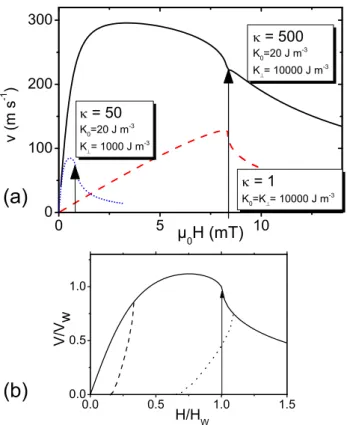
The resulting calculated v(H) curve of ideally prop-agating DWs is shown in Fig. 3a for various values of K0, K_⊥. The dependence of the maximum velocity on

the magnetic anisotropies can be understood as follows for transverse DWs. When the field is applied along the easy axis, the DW magnetization starts precessing around it and comes out of the plane by an angle φ. The resulting magnetostatic charges created at the surfaces of the layer create a demagnetizing field Hdemag:

propor-tional to Ms in soft in-plane magnetized materials such

as Py, or to the uniaxial anisotropy field 2K_⊥/µ0Ms in

the case of in-plane magnetization induced by magneto-crystalline anisotropy. It is the torque between Hdemag

and the DW’s magnetization that propels the DW for-ward with a velocity proportionnal to Hdemagand ∆(φ).

As the applied field increases, so does φ, resulting in the progressive shrinking of the DW width from its static value, becoming: ∆(φ)=_√ ∆0

1+κsin2

φ. At small κ, this

non-linearity is minor, and the mobility is linear up to Walker breakdown (κ=1 curve in Fig. 3a). As κ in-creases, the end of the stationary regime evolves into a broad plateau. Its amplitude rises with increasing out-of-plane anisotropy coefficient K_⊥ (through its effect on Hdemag), but also with decreasing in-plane anisotropy

as this will broaden the DW, and increase the veloc-ity. The 1/√K0 dependence of the velocity is however

4

FIG. 2. (a) Domain wall velocity for the [Mn]ef f=4.7%

sam-ple at T =25, 60 and 85 K. (b) Modification of the domain profile with increasing field.

of κ ≫1, the expression of the maximum velocity can in fact be simplified to V∞ max ≈ 2γ Ms √ AexcK_⊥,

evidenc-ing once more the weaker influence of the uniaxial in-plane anisotropy on the maximum speed. In Permalloy nanowires, the magnetic anisotropy mainly results from the shape of the wire, and typical κ are close to 1. In our samples on the contrary, κ=20-200 (Table I).

In the framework of this model, and taking into ac-count that the DWs depin at a finite field (very close to the coercive field) two different experimental scenarios can occur as shown schematically in Fig. 3b: the DW propagation can meet the intrinsic regime either before (dashed line) or after (dotted line) the Walker field. We attribute samples A3, A4 to the first category, and sam-ples B3, C3 to the second one.

For samples with very low anisotropy fields (B3, C3), the Walker field is expected to be quite small, and the DW velocity meets directly the precessional regime (dot-ted line in Fig. 3b), at which point the velocity decreases with field. An upper boundary for the damping constant can then be estimated from HW=αK⊥/µ0MS. Using

the anisotropy coefficients determined by FMR and the experimental peak fields Hmax at different temperatures

(Table I) then yields αmax=0.02-0.04. This value is very

much of the order found by variable-frequency FMR28_,

but ten times smaller than the one estimated from the ra-tio of stara-tionary and precessional mobilities (µstat, µprec)

in out-of-plane magnetized GaMnAs9_{. Although this}

dis-crepancy has been pointed out before29_{, it may also}

orig-inate from an incorrect evaluation of µstat in these

sam-ples. Finally, calculating the field expected to give the maximum velocity at T ≈0.2Tc gives: µ0Hmax=1.2 mT

(1.5 mT) for sample C3 (B3). These are barely above their coercive fields µ0Hc=0.9 mT (1.2 mT), which

ex-plains why the high velocity plateau is not seen at all. For samples with higher anisotropy fields (A3, A4), it is the stationary regime that is reached after depinning (dashed line in Fig. 3b). This occurs at exceptionally high speeds (≈ 150 m s−1 _{for A3 and ≈ 300 m s}−1 _for

A4) which contrasts strongly with the claims of Ref. 11 of a stationary regime reached by 8.10−2 _{m s}−1_{. The}

expected saturation velocities calculated from Eq. (1) at

T ≈0.2Tc from the 1D model are indicated in Table I for

samples A3 and A4. For this calculation, the exchange constant was taken as 3.10−13 _{J m}−1 _{for [Mn]ef f=4.7%}

(sample A4) and as 10−13_{J m}−1_{for [Mn]ef f=3.7%}

(sam-ple A3), as estimated on perpendicularly magnetized samples of similar manganese content7_{. The}

experimen-tally determined velocities follow the predicted trend of increasing Vmax with perpendicular anisotropy K⊥, as

well as the weaker influence of the in-plane anisotropies (Table I). However, the observed maximum velocities are underestimated by a factor of about 1.5, and the velocity plateaus are unexpected within this model. As evidenced repeatedly in both simulations3 _{and experiments}30_{, an}

abrupt change in velocity often results from a modifi-cation of the nature of the DW. A modifimodifi-cation of the domain profile can indeed be seen on the domain images of samples A3 and A4 (Fig. 2b). The domain gradually loses its sawtooth shape and smoothens out with increas-ing field, or more exactly divides up into sawtooths of shorter period. These DW transformations could be the reason for the plateaus observed for samples A3 and A4. To summarize, the 1D model provides gives good quali-tative trends, but underestimates the observed velocities, possibly due to a transformation of the DW profile.

0 5 10 0 100 200 300 = 50 K 0 =20 J m -3 K= 1000 J m -3 = 500 K 0 =20 J m -3 K= 10000 J m -3 µ 0 H (mT) = 1 K 0 =K= 10000 J m -3 v ( m s -1 ) 0.0 0.5 1.0 1.5 0.0 0.5 1.0 H/H W V / V w (b) (a)

FIG. 3. Computed 1D model v(H) curves with the vertical arrows indicating the position of the Walker field. (a) Vary-ing in-plane (K0) and out-of-plane (K_⊥) anisotropies without

pinning (following Ref. 3 with α=0.03, Aexc=10−13J m−1,

Ms=36 kA m−1). (b) Possible modifications to the v(H)

curve when pinning is taken into account. The DW veloc-ity may rejoin the intrinsic regime before Walker breakdown (dashed line) or afterwards (dotted line).

This work gives clear guidelines for designing high speed DW based devices. In particular, the largest DW velocities are found for 180◦ _{charged DWs propagating}

along the easy axis, with layers exhibiting the largest out-of-plane anisotropy and a weak in-plane anisotropy, which corresponds to a large DW width. Lateral con-finement of the DWs through nanostructuration of the layer is expected to have a further impact on the

max-imum velocity since it will affect the uniaxial in-plane anisotropy, as already shown in GaMnAs31_{. In light of}

our results, this additional parameter would open a wide range of possibilities to control the DW dynamics in field-or current- driven DW motion experiments.

We acknowledge C. Dor´e and S. Majrab for technical assistance. This work was performed in the framework of the MANGAS project (ANR 2010-BLANC-0424-02).

1

S. S. P. Parkin, M. Hayashi, and L. Thomas, Science 320_{, 190 (2008).}

2

H. T. Zeng_{, D. Read, L. OBrien, J. Sampaio, E. R.} Lewis, D. Petit, and R. P. Cowburn, Appl. Phys. Lett. 96_{, 262510 (2010).}

3

A. Thiaville_{and Y. Nakatani, Spin Dynamics in} Con-fined Magnetic Structures III, p. 183, Springer, New York, 2006.

4

R. Moriya_{, M. Hayashi, L. Thomas, C. Rettner, and} S. S. P. Parkin_{, Appl. Phys. Lett. 97, 142506 (2010).}

5

K. Yamada, J.-P. Jamet, Y. Nakatani, A. Mougin, A. Thiaville_{, T. Ono, and J. Ferr´}e_{, Appl. Phys. Expr.} 4_{, 113001 (2011).}

6

S. Middelhoek, IBM J. Res. Dev. 10, 351 (1966).

7

S. Haghgoo, M. Cubukcu, H. von Bardeleben, L. Thevenard_{, A. Lemaˆıtre, and C. Gourdon, Phys.} Rev. B 82, 041301(R) (2010).

8

L. Thevenard, L. Largeau, O. Mauguin, A. Lemaˆıtre_{, K. Khazen, and H. von Bardeleben,} Phys. Rev. B 75, 195218 (2007).

9

A. Dourlat, V. Jeudy, A. Lemaˆıtre, and C. Gourdon, Phys. Rev. B 78, 161303 (2008).

10

L. Herrera Diez_{, J. Honolka, K. Kern, E. Placidi,} F. Arciprete, A. W. Rushforth, R. Campion, and B. Gallagher_{, Phys. Rev. B 81, 094412 (2010).}

11

H. Tang_, R. Kawakami_, D. Awschalom_{, and} M. Roukes, Phys. Rev. B 74, 041310(R) (2006).

12

A. Sugawara, H. Kasai, a. Tonomura, P. Brown, R. Campion_{, K. Edmonds, B. Gallagher, J. Zemen,} and T. Jungwirth, Phys. Rev. Lett. 100, 1 (2008).

13

N. L. Schryer and L. R. Walker, J. Appl. Phys. 45, 5406 (1974).

14

A. Malozemoff_{and J. Slonczewski, Phys. Rev. Lett.} 29_{, 952 (1972).}

15

M. Cubukcu_{, H. J. von Bardeleben, K. Khazen, J. L.} Cantin_{, O. Mauguin, L. Largeau, and A. Lemaˆıtre,} Phys. Rev. B 81, 41202 (2010).

16

Please refer to Supplemental Materials for details.

17

A. Lemaˆıtre_{, A. Miard, L. Travers, O. Mauguin,} L. Largeau, C. Gourdon, V. Jeudy, M. Tran, and J. George, Appl. Phys. Lett. 93, 21123 (2008).

18

A. Hubert_{and R. Sch¨}afer_{, Magnetic domains, Berlin,} Springer edition, 2000.

19

S. Corodeanu, H. Chiriac, and T.-A. Ovari, Rev. Sci. Instr. 82, 094701 (2011).

20

U. Welp_{, V. K. Vlasko-Vlasov, X. Liu, J. K.} Fur-dyna, and T. Wojtowicz, Phys. Rev. Lett. 90, 167206 (2003).

21

J. Honolka_{, L. Herrera Diez, R. K. Kremer,} K. Kern, E. Placidi, and F. Arciprete, New J. Phys. 12_{, 093022 (2010).}

22

L. Finzi and J. Hartman, IEEE Trans. Mag. 4, 662 (1968).

23

W. Lee_{, B.-C. Choi, Y. Xu, and J. Bland, Phys. Rev.} B 60, 10216 (1999).

24

M. Hayashi, L. Thomas, C. Rettner, R. Moriya, and S. S. P. Parkin_{, Nat. Phys. 3, 21 (2006).}

25

L. Thevenard_{, C. Gourdon, S. Haghgoo, J. P. Adam,} H. von Bardeleben, A. Lemaˆıtre, W. Schoch, and A. Thiaville_{, Phys. Rev. B 83, 245211 (2011).}

26

J. P. Adam_{, N. Vernier, J. Ferr´}e_{, A. Thiaville,} V. Jeudy, A. Lemaˆıtre, L. Thevenard, and G. Faini, Phys. Rev. B 80, 193204 (2009).

27

C. Zinoni_{, A. Vanhaverbeke, P. Eib, G. Salis, and} R. Allenspach, Phys. Rev. Lett. 107, 207204 (2011).

28

K. Khazen, H. von Bardeleben, M. Cubukcu, J. Cantin_{, V. Novak, K. Olejnik, M. Cukr, L.} Theve-nard, and A. Lemaˆıtre, Phys. Rev. B 78, 1 (2008).

29

G. Vella-Coleiro, Appl. Phys. Lett. 21, 36 (1972).

30

M. Kl¨aui_{, P.-O. Jubert, R. Allenspach, A. Bischof,} J. Bland_{, G. Faini, U. R¨}udiger_{, C. Vaz, L. Vila, and} C. Vouille, Phys. Rev. Lett. 95, 026601 (2005).

31

J. Wenisch_{, C. Gould, L. Ebel, J. Storz, K. Pappert,} M. J. Schmidt_{, C. Kumpf, G. Schmidt, K. Brunner,} and L. W. Molenkamp, Phys. Rev. Lett. 99 (2007).