-A
Complete Characterization of Optical Pulses
in the Picosecond Regime for Ultrafast Communication
Systems
by
Jade P. Wang
Submitted to the Department of Electrical Engineering and Computer Science in partial fulfillment of the requirements for the degree of Master of Engineering in Electrical Engineering and Computer Science
at the
MASSACHUSETTS INSTITUTE OF TECHNOLOGY
August 2002
@
Massachusetts Institute of Technology, 2002. All rights reservedMASSACHUSETTS INSTITUTE OF TECHNOLOGY
JUL 3 0 2003
LIBRARIES V, Certified by......-fDepart'rrisfit of Electrical Engineering and Computer Science August 21, 2002
...
Erich P. Ippen Elihu Thomson Professor of Electrical Engineering Thesis Supervisor
Certified by... ...
Scott A. Hamilton MIT Lincoln Laboratory Staff Member
T)p6s Supervisor Accepted by...
Arthur C. Smith Chairman, Deparment Committee on Graduate Theses Author..
Complete Characterization of Optical Pulses
in the Picosecond Regime for Ultrafast Communication
Systems
by
Jade P. Wang
Submitted to the Department of Electrical Engineering and Computer Science in partial fulfillment of the requirements for the degree of Master of Engineering in Electrical Engineering and Computer Science
Abstract
Ultrashort optical pulses have a variety of applications, one of which is the develop-ment of optical time-devision multiplexing (OTDM) networks. Data is encoded in these short optical pulses (typically a few picoseconds in length) which are then inter-leaved in time to provide very high data rates on a single wavelength. Wavelength-division multiplexing (WDM) uses multiple channels by interleaving pulses in fre-quency in order to achieve high data rates. Typical pulse lengths in WDM are on the order of hundreds of picoseconds. OTDM networks have some advantages over WDM networks, but in order to take advantage of these characteristics, a better understanding of short optical pulse characterization needs to be reached. Such in-vestigation requires accurate pulse characterization in the form of amplitude and phase measurements. Traditional methods of measurement such as nonlinear opti-cal autocorrelation and spectral analysis cannot accurately measure pulse shape and phase. Two new methods of accurate characterization of amplitude and phase are frequency-resolved optical gating (FROG) developed by Rick Trebino, and a spectral interferometric method developed by Jean Debeau. The second-harmonic generation FROG method is highly sensitive but works best for femtosecond pulse lengths, due to the need for large spectrum. The spectral interferometric method is straightfor-ward to implement using common fiber-coupled components, but suffers from a need for high pulse-to-pulse coherency, which implies that it is less practical for actual communication networks.
Thesis Supervisor: Erich P. Ippen
Title: Elihu Thomson Professor of Electrical Engineering Thesis Supervisor: Scott A. Hamilton
Acknowledgments
First of all, I would like to thank my colleagues at the MIT Lincoln Laboratory, who have all been extremely patient and helpful in dealing with my many questions. My thesis advisor, Professor Erich Ippen, has been indispensable in helping me see this project to its end. Whenever some particularly recalcitrant problem has come up in the course of my experiments, he has always had the ability to see another path towards the eventual goal. My research supervisor, Dr. Scott Hamilton, always takes the time out to explain things thoroughly to me and taught me all the basics of working in a fiber optics lab. His guidance on this project has kept it alive far past the point when I would have been unable to proceed any further. Finally, his ability to successfully finish four things at once while still finding the time to help me with my work is very inspiring-and impressive.
Soon-to-be Dr. Bryan Robinson was also invaluable in his ability to mesh his practical knowledge of the laboratory with a sound mathematical and theoretical foundation. Without his help during the last few weeks, I could not have possibly finished this thesis. Shelby Savage, another student in the laboratory, was also ex-tremely helpful in explaining difficult concepts in ways that I could understand. He would also often keep me sane during particularly frustrating bouts with the auto-correlator by providing a much-needed sense of humor. I would also like to thank Thomas Murphy, who was always happy to answer even the most trifling questions. I would also like to thank him particularly for putting up with me as an office mate. Steve Constantine has always encouraged me and made the impossible seem possible again. Todd Ulmer has always encouraged me by making me realize that things could always be worse. I would also like to thank Professor James K. Roberge, for showing me that I could do great things, and for believing in my abilities when I had doubts.
I would also like to thank my family and my friends from MIT and elsewhere,
without whom I might have still finished this thesis but I certainly would not have finished it sane. My mother and father have always believed in my ability to finish what I begin, and to do it well. My brother has always been a source of encouragement to me, despite having grown apart these few years. I would like to thank my friends Keith Santarelli, for being an inspiration to me throughout my MIT career; Laura Kwinn and Sammi Truong for being able to put up with me as a roomate; Jennifer Chung, who is a great housemate and can always make me laugh; Edwin Karat, my generous housemate who had the dubious distinction of being pestered with a variety of technical questions and whose books were always extremely helpful; Emily Marcus, Laura Cerritelli, Susan Born, Jamie Morris, and Michelle Goldberg for always being ready to cheer me up; Karen Robinson and Juhi Chandalia for helping me through Nonlinear Optics and for the various fascinating conversations on our chosen field; Natalie Garner and Phil for showing me that there was more to life than nonlinear optics; and finally Jay Muchnij for being willing to listen to me past the point when any normal person would have fallen asleep. Finally, I would like to thank the denizens of the zephyr instance help, for their invaluable help in dealing with LaTeX.
Contents
1 Introduction
2 Pulse Propagation Theory
2.1 Nonlinear Polarization . . . . 2.1.1 Intensity Dependent Index of Refraction . . . 2.2 Wave propagation in Fibers . . . .
2.3 The Nonlinear Schr6dinger Equation . . . .
3 FROG Pulse Characterization Theory
3.1 Autocorrelation . . . .
3.2 Spectral Measurements . . . .
3.3 Frequency-Resolved Optical Gating . . . .
3.3.1 Methods for Obtaining a Trace . . . . 3.3.2 Simulations of FROG Traces . . . .
3.3.3 Extracting Phase and Amplitude . . . .
4 Interferometric Pulse Characterization Theory
5 Pulse Characterization Experiment and Analysis 5.1 Measurement Methodology . . . . 7 13 . . . . 17 . . . . 22 . . . . 29 . . . . 34 39 . . . . 40 . . . . 43 . . . . 45 . . . . 48 . . . . 49 . . . . 51 55 71 75
5.2 Verification and Calibration . . . . 76
5.2.1 Simple Optical Pulse Source . . . . 76
5.2.2 Pulse Characterization Experiment . . . . 79
5.3 Practical Optical Pulse Sources . . . . 87
6 Conclusions and Future Work 95
Chapter 1
Introduction
Currently, there is a need, for a variety of applications, to create shorter and more precisely characterized optical pulses. Such pulses have large bandwidths, and thus are useful for material characterization via spectroscopy. Ultrashort pulses can be useful in imaging extremely fast temporal effects such as molecular rotations via "time strobing".' They are also useful in the field of medicine, whether in examining structures or performing surgery2 without invading the body. For spectroscopic ma-terial characterization and temporal sampling, the optical pulsewidth is typically a few femtoseconds or less. Finally, short pulses are also necessary for the development of optical time-division multiplexing (OTDM) networks. In such networks, data is encoded in short optical pulses (typically a few picoseconds in length) which are then interleaved in time. This provides very high aggregate data rates in a single chan-nel. Another method, wavelength-division multiplexing (WDM), interleaves pulse trains in frequency to achieve high data rates using multiple channels. The optical pulsewidths used in WDM systems today are typically hundreds of picoseconds long.
Recently, both OTDM and WDM fiber transmission links have been demonstrated at data rates exceeding one terabit/second.'-' Because such data rates are several or-ders of magnitude greater than electronic processing speeds, architecture for such systems must be carefully considered in order to implement extremely capable op-tical networks in the future. Most networks in use today are WDM networks, due to relative commercial component maturity, but OTDM networks have several po-tential advantages.6 For instance, OTDM networks can simultaneously provide both
guarenteed bandwidth and truly flexible bandwidth on demand service if slotted or packetized transmission is used. Network management and control are also easier to understand and to implement due to the single channel nature of the data. Further-more, such networks are ideally suited to statistical multiplexing of data and much more scalable in the number of uses than WDM networks. However, in order to take advantage of these characteristics, several difficulties related to short optical pulse transmission need to be overcome. These difficulties include noise accumulation, the presence of group velocity dispersion (GVD), polarization-mode dispersion, and ma-terial nonlinearities. Investigation and ultimately control of these effects in ultrafast optical communication systems requires an accurate way of measuring short pulses that are a few picoseconds in length.
Traditional methods of measuring pulses include using the optical autocorrelation and the spectrum of the pulse in order to estimate the pulse width and shape. Optical autocorrelation is a technique in which the pulse under test is used to sample itself. However, due to the symmetric response, the autocorrelation is incapable of providing insight as to pulse envelope asymmetry or frequency chirping. Furthermore, the esti-mation of the pulse width is based upon an assumed pulse envelope shape, which may or may not be correct. Optical pulse characterization inferred from autocorrelation
measurements is not only inaccurate due to errors between the measured and assumed pulse shape, but incomplete because only temporal information is considered.
Complete characterization in the time or frequency domain requires both magni-tude and phase (or temporal and spectral profile) of a pulse. With both temporal and spectral information, it is possible to determine the pulse characteristics completely, since spectral content is related to temporal content through the properties of the Fourier transform. However, in any measurement, we can only obtain temporal or spectral intensity of the signal. Pulse characterization is complicated further by the existence of chirp. The instantaneous frequency of a chirped pulse varies across the pulse, which means that the pulse is not transform-limited. Transform-limited pulses allow us to make assumptions about the relations between the spectral and temporal information of a pulse which can make characterization simpler.
There are several pulse characterization techniques which have been developed to completely determine pulse phase and magnitude. Interferometric techniques, which analyze the coherent interference between two copies of the pulse, are most effec-tive in the nanosecond range. Another technique, called FROG (frequency-resolved optical gating), is aimed at femtosecond pulses with large bandwidths. For our sys-tems, however, we need to characterize pulses in the picosecond regime. Picosecond pulses are particularly difficult to characterize, since they do not have the large band-width of femtosecond pulses, nor do they have the accessible temporal information of nanosecond pulses.
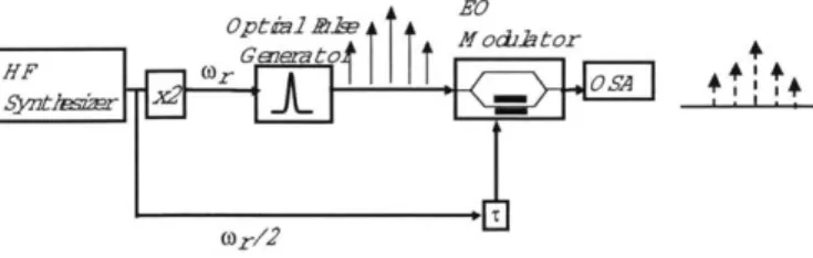
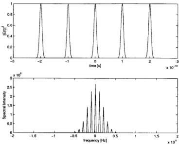
An interferometric method developed by Jean Debeau7 has been demonstrated for picosecond pulse characterization. This method uses an electro-optic modulator to modulate the pulse train of interest at half the frequency of the pulse train. As
a result, the spectral lines of the pulse train of interest are mixed down and up into new spectral lines. Since each new spectral line contains information from exactly two adjacent original spectral lines, it is possible to extract the relative phases of the original spectral lines from the new spectral lines. Using picosecond width pulses at high repetition rates and a high-resolution spectrometer, it is possible to measure the phase of the pulses in the pulse train. This method uses common fiber-coupled equip-ment, making for a simple setup. Furthermore, it provides a method of measuring the phase profile of a pulse directly, without resorting to iterative algorithms. However, one large drawback which limits the generality of this method is the need for high pulse-to-pulse coherency in the pulse train of interest. This limits the generality of this method severely.
The frequency-resolved optical gating (FROG)8-13 method relies upon
simultane-ously measuring the temporal and spectral pulse content, which is then displayed as a spectrogram. Using an iterative algorithm to characterize the measured spectrogram, we can then accurately determine the pulse amplitude, phase, and frequency chirp. Currently, a variety of FROG methods have been developed, including polarization-gate (PG) FROG, self-diffraction (SD) FROG, transient-grating (TG) FROG, second harmonic generation (SHG) FROG, and third harmonic generation (THG) FROG. Another method, the sonogram, involves finding the spectrogram in a way which is essentially the reverse of the FROG method.
Chapter 2 presents the theory behind pulse propagation in fibers, including dis-persion, the nonlinear index of refraction, and the nonlinear Schr6dinger equation. In preparation for later chapters, pulse distortion and its causes will also be discussed.
its advantages and disadvantages for the picosecond regime. Simulations of FROG traces using second harmonic generation (SHG) FROG will be presented. Finally, we will close with a discussion on the algorithm for extracting the phase and amplitude of a pulse.
Chapter 4 will present the theory of interferometric pulse characterization and its advantages and disadvantages over the FROG method for the picosecond regime. Simulations of pulse characterization experiments will be presented for comparison with results shown in Chapter 5.
Chapter 5 will detail the experimental efforts in implementing a system which can completely characterize picosecond pulses. Results of the experiments will be
analyzed and compared to simulations shown previously in Chapter 4.
Chapter 6 summarizes the conclusions of this thesis and provides suggestions for future work in this area.
Chapter
2
Pulse Propagation Theory
In fiber communication systems, short optical pulses are used to transmit data, with a variety of encoding schemes including return-to-zero (for OTDM) and non-return-to-zero (WDM). For simplicity, we consider an optical field as a superposition of monochromatic plane waves traveling in the z direction1 4
3
E(z, t) = 6i
I
[Ei(wa)ei(kiz-wat) +c.c.1.
(2.1)Wa i=1
Here, the sum over Wa sums over all frequencies. The second sum, over i, includes all three possible polarizations of the plane waves. We also define the intensity as the magnitude of the time averaged Poynting vector:
I =ceE(t)|2 "') (2.2)
2
where we have dropped the spatial dependence for simplicity.
this case, we can assume our electric field at a particular frequency w can be written as a combination of a slowly-varying envelope (A(r, t)) and a plane wave. This is a common representation for optical pulses as used in communication systems.
E(w, z, t) = BA(r, t)e(kzwot).23)
We drop the spatial dependence for simplicity and add a phase term,
E(wo, t) = BA(t)e-i(Wot+e(t)). (2.4)
Instantaneous frequency is defined as
dqp(t)
Winst = Wo + dt. (2.5)
For optical pulses, a useful term is chirp, which is defined as the second derivative of the phase of the pulse, or the first derivative of the instantaneous frequency.
chirp - dt dt) (2.6)
dt dt2
We can expand Equation (2.4)
E(w0, t) = 8A(t)e-(Wot+Co+C1t+C2t2
+C3t3+...). (2.7)
Here, we have explicitly written out the possible forms of the time-dependent phase.
CO and C1 are coefficients for zero chirp. C2 is the coefficient for constant chirp, C3
is the coefficient for linearly time-varying chirp, and so on.
When the pulse instantaneous frequency is constant, the pulse varies linearly with time and the pulse is described as having zero chirp. Constant chirp occurs when the pulse phase is quadratic and the pulse instantaneous frequency therefore varies linearly with time. Linear chirp occurs when the pulse phase is cubic and the instan-taneous frequency is quadratic. Higher order instaninstan-taneous frequency dependence results in nonlinear chirp.
The presence of chirp in a pulse is typically induced both by dispersion and by non-linearities in the medium through which the pulse propagates. nonlinearly induced chirp in a pulse increases its temporal broadening rate when the pulse propagates through a dispersive media. It can also cause a spectral broadening in the pulse with-out changing its intensity profile, thus causing problems for communications systems which rely on efficient use of bandwidth. Furthermore, without the ability to char-acterize the chirp of a pulse, it is much more difficult to predict how a given pulse will change envelope shape and width as it propagates. Figure 2.1 shows an example of a Gaussian pulse with constant chirp (quadratic phase) compared to an unchirped pulse. This comparison illustrates the effect of chirp on the bandwidth of a pulse.
Let us take a look at some common forms for the pulse envelopes (A(t)) as de-scribed in Equation (2.4)). A Gaussian envelope is of the form
t2
E(t) = Be-r , (2.8)
where B is a constant amplitude and T is the half-width at the 1/e intensity point of the pulse. The more common measure of pulse width is the full-width at half-maximum (FWHM). Both T and the FWHM are measured with regard to the intensity
0.5 -50 0 50 (a) Time [fs] 1 [pi 1 I A ( AA -- E(t)
|
0.5 | - -- (t) | 0.5 -50 0 50 (c) Time [fs] 0.5- 0-0 200 400 600 (e) Frequency [THz] :-0.5 -50 0 50 (b) Time [fs] 1 200 E(t) 0 . 100 -50 0 50 (d) Time [fs] 1- 0.5-0 200 400 600 (f) Frequency [THz]Figure 2.1: (a) and (b) show the intensity of the unchirped Gaussian and the chirped Gaussian, respectively. Note that they are identical. (c) shows the electric field of the unchirped Gaussian and the phase of the unchirped Gaussian. (d) shows the electric field and phase for a Gaussian of the same FWHM with constant chirp. (e) and (f) show the corresponding spectral intensities for the two Gaussians. For these plots, the FWHM is 20 fs. The quadratic chirp is 0.02 [rad/fs2].
(fig/exgausschirps2.eps)
of the Gaussian pulse, given by
1(t) = I 2e$, (2.9)
where I, = "B 2. The FWHM is related to
T by the following relation
102
FWHM = 2T/n 2. (2.10)
fiber lasers and diode lasers. A hyperbolic secant (sech) pulse envelope is the natural solution to the soliton equations. For more information on solitons, please refer to Chapter 5 of Agrawal.1 5 Sech pulses take the form
t
E(t) = Bsech , (2.11)
TO
where B is the amplitude of the pulse, and To is related to the full-width at half maximum by
FWHM = 2TO ln (1 + v'2). (2.12)
The full-width at half maximum is measured from the intensity envelope of the pulse. Figure 2.2 plots the intensities of a gaussian and a sech pulse, both with a full width at half maximum of 2 ps.
2.1
Nonlinear Polarization
Thus far, we have only considered electric fields in free space. Let us next consider how electromagnetic waves act within materials. We first consider a dielectric material. When an electric field is applied, the dielectric material polarizes and a polarization current is induced. This material polarization leads to a linear change in the index of refraction of the material as well as higher order nonlinear terms which act as new sources of electromagnetic radiation. The relation between the electric displacement
D, the electric field E and the electric polarization P is
1 0.9 0.8 0.7 0.6 ci)S0.5 0.4 0.3 0.2 0.1 -4 -3 -2 -1 0 t [S] Figure 2.2: Example of an max of 2 ps (solid line) and max (dotted line).
1 2 3 4
x 1012
unchirped gaussian pulse with a full-width unchirped sech pulse with same full-width half-(fig/gausssech.eps)
The electric polarization of a dielectric material is defined to be the sum of the electric dipole moments per unit volume induced in the material by the presence of an electric field.16 These electric dipole moments are induced over time scales defined by
molecular, ionic, and electronic processes in the material. In silica fiber, the electronic effects dominate, which results in a nearly instantaneous response of approximately
10 fs.
The induced material polarization can be expanded into linear and nonlinear terms
(2.14) P(r, t) = pL (r, t) + pNL (,t
where
pL (rt) P(1)(r, t) (2.15)
and
PNL(r t) p( 2)(r, t) + p(3)(r, t) + p(4)(r, t) +
.... (2.16)
Using Fourier analysis, we can expand the polarization in an infinite sum of sepa-rate frequency components, similar to our earlier treatment of the electric field in Equation (2.1).
P(")(r, t) = 1 P(n)(rwb)ei(kbr-Wbt) + c.c.1. (2.17)
Wb i
Again, we first sum over frequencies and then sum over all possible polarizations. An example of a polarization P ()(r, wn), for the case when only sum frequencies are included, is
P(r, wm) = E (X (1) (Wm = wI) E(wi) + X(2)(Pm = wI + w2) E(wi)E(w2) (2.18) + X(3)(Wm = Wi + W2 + w3) : E(wi)E(w2)E(w3) + ...)
- P(I) (r, Wm) + p(2) (r, wi) + p(3) (r, WM) + .. ,
where the X's are the nonlinear susceptibilities. As a result of the vector nature of the electric field and polarization, the susceptibility is a tensor quality. The susceptibility of order n for nth order polarization and field is a tensor of order n + 1. To illustrate the tensor nature of this term, we can explicity write out the third-order material
polarization in terms of the electric field and susceptibility: p3)
[P
3(w)
p(3) (3) x () (3)Lxxx
(3) Xxxxy (3) Xyxxy (3) Xzxxy S xzzz .. Xyzzz .. XZZZZj E.(wi) E.(wi) E.(wi) E.(wi) Ez(wi) Ez(wi) It is clear that the x tensor is a fourth-ordersummation form as follows:
tensor. We can also write this in a
Pf(W =Wo + Wn + Wm)=
o Xjkl ( = wo + wn + Wm : WoW n,W m)Ej (Wo)Ek (Wn)E(Wm). (2.20) jkl (mno)
We include the second summation, over (mno) to illustrate that the material po-larization at a frequency w only requires the frequency components of the relevant electric fields to sum up to w. Thus, m,n,and o may take on any number as long as their sum gives us the correct frequency component for the material polarization. In general, the calculation of the material polarization is greatly simplified by the fact that due to symmetry conditions in many materials, many of the quantities in the X
tensors are zero.
In fiber, the second order susceptibility is negligible due to the symmetries of silica glass. As a result, fiber nonlinearities are mainly due to third order effects. Let us
E.(w2) E.(w2) E2(w2) E. (w2) Ez(w2) Ez(w2) E.(W3) Ey(w3) Ez(w3) E. (W3) Ey(w3) E,(w3)_ (2.19)
consider the third order polarization, for an incident electric field with three frequency components. In a more general case when an optical pulse is considered, the incident electric field often consists of many more frequency components. We assume that each of the electric field components are polarized in the same direction and drop the space dependence in the following equations for simplicity. From Equation (2.1), we obtain
E(w) (E(wi)eiwl + E(w2)ew + E(w3)e ± c.c.). (2.21)
The frequencies present in the material polarization will be third-order combinations of the frequencies present in the electric field. Thus, if we calculate E(t)3, we can
observe which frequencies will be present in the material polarization.
E(a)3 ( E(wi)e-w't + E(w2)e-iw2t + E(w3)e-iw3t + c.c. (2.22)
= (E(wi)3e-3iwit + E(wi)2E*(wi)e-iwl + 2E(wi)E(w2)E*(3)egw1±w me-a3)t +
From this, we see that all sum and difference combinations of its frequencies wi,omega2,
and w3 are possible. We can write the polarization in terms of its separate frequencies by looking at the Fourier transform. Thus, each frequency of the polarization
corre-sponds to some combination of the incident E fields. There are 44 separate frequency components, the Fourier transform sum of these 44 separate components results in the total polarization. A few of the specific frequency components are written out
below.
P(wi) =
±X(3)
(3E(wi)E* (wi) + 6E(w2)E*(w2) + 6E(w3)E*(w3))E(wi) (2.23)4
P(3wi) = (3)E3(W1) (2.24)
P(wi + w2 + w3) = X(3)E(wi)E(W2)E(W3) (2.25) P(2w2 - w) = X(3)E(w2)2E*(wi) (2.26)
4
A more complete listing can be found in Boyd" (Boyd uses a slightly different
nota-tion).
The various contributions to the nonlinear polarizations are results of particular nonlinear processes. For example, second harmonic generation and sum harmonic generation are generated by second order X(2) nonlinearity, while self- and cross-phase modulation, four-wave mixing, and Raman scattering are examples of third order X(3) nonlinearity. Observable electric fields are always real and thus have both positive and negative frequencies associated with them. Mixtures of negative and positive frequencies in the mathematics help explain nonlinear phenomena such as the optical Kerr effect, optical rectification, and coherent anti-Stokes Raman scattering.
2.1.1
Intensity Dependent Index of Refraction
The material polarization as described above can cause nonlinear effects, especially in isotropic materials such as silica glass, where third-order effects dominate. One such effect is the intensity dependent index of refraction which can often cause distortions in optical pulses as they propagate through fiber. The intensity dependent index of refraction can be caused by either self-phase modulation (SPM) or cross-phase
modulation(XPM). In self-phase modulation, a pulse propagating in fiber induces an intensity-dependent nonlinear change in the index of refraction of the fiber. In cross-phase modulation, a second field causes an intensity-dependent nonlinear index of refraction experienced by the first field. These effects result from third order processes which are dominant in fiber since silica glass is isotropic. Thus, for fiber, we can write
D(w) = c (I + X)(w) )E(w) + P(3)(w), (2.27)
where p(3) (w) can be expanded in the same way as in Equation 2.20. The index of refraction in the absence of nonlinear polarization is defined to be
nor= 1+ X)(w). (2.28)
Let us first consider the case of self-phase modulation in fiber. We assume an incident electric field at a single frequency w
1 2
As stated before, self-phase modulation will cause a change in the index of refraction observed by the electric field. We define a new index of refraction as
n = no + An, (2.30)
where An is the change caused by SPM. To solve for An, we consider the nonlinear polarization in Equation (2.27). For self-phase modulation, the relevant third-order material polarization term is that which occurs at the same frequency as the incident
field and with the same polarization.
P () _ 3) (u;:w, w, -w)E1(w)E1(w)E*(-w) (2.31)
+ X$2(w 3 : w, -w, w) El(w) E*(-w) El(w)
+ (3) : -w, w,w)E*(-w)E1(w)E1(w)}.
Due to intrinsic permutation symmetry, we can interchange the frequency arguments at the same time we interchange the cartesian indices. In our case, the cartesian indices are all the same. As a result, we can sum all three terms, which gives us a coefficient of 3. Rewriting Equation (2.27) for self-phase modulation in fiber we obtain
Dx(w) = co(1 + X9(w))E1(w) + 3o X ()x(w)IEl(w)12El(w). (2.32)
4
We can rewrite Equation (2.32)
Dx(w) = co(1 + XM9(W) + ( (2.33)
4
Using Equations (2.28), (2.30) and (2.32), we can see that
n2 = (no + An)2 = (1 + X9(1) +
( x (w)IEl(w)12).
(2.34)
4
We find that the change in the index of refraction is both nonlinear and proportional to the intensity of the field. Let us define An to be n2', where n2 is a constant of
proportionality. Thus, Equation (2.30) becomes
where I is defined (from Equation (2.2)) as
I noccl E1(w)12. (2.36)
We now solve for n2. Substituting Equation (2.35) into Equation (2.34), we obtain
(n2 + 2non2I + n 2I 2) = 1 +
XM(w)
+ 4Xxx
(w)IE1 (w) 2. (2.37)Since n2 is typically very small, n I2 is negligible and can be neglected.
Further-more, we can also cancel out several terms by substituting in Equation (2.28), finally obtaining
3
2non21 = -X$3 x (w)IEl(w)12. (2.38)
4
Substituting Equation (2.36) into Equation (2.38) and solving for n2, we obtain
n2 = C X2x(w). (2.39)
We see from Equation (2.39) that self-phase modulation causes a change in the index of refraction proportional to the intensity of the field. This implies that an intensity-dependent phase shift will be induced upon the field. In the case of propagating pulses, the phase shift induced upon the pulse is dependent on the pulse intensity, which varies across the pulse envelope. In other words, the pulse will acquire increased
bandwidth as well as chirp as it propagates.
The derivation of self-phase modulation derived here was for a linearly-polarized field. For a circularly polarized field, the constant of proportionality n2 is 2 that for
index of refraction, let us briefly consider n2 for phase modulation. In
cross-phase modulation, a strong field (pump) can affect the index of refraction seen by a second, weaker field (probe) in much the same way as a field can affect itself in SPM. In order to calculate n2 for a XPM effect, we must first realize that there are several
different types of cross-phase modulation.
1. The pump is of the same polarization as the probe, but of different frequency.
2. The pump is of different polarization than the probe, but is of the same fre-quency.
3. The pump is of the same polarization and same frequency as the probe, but is
sent in at a different angle from the probe to distiguish the two fields from each other.
4. The pump and probe are circularly polarized instead of linearly polarized.
Let us consider cross-phase modulation in the case where the pump and probe have the same (linear) polarization but different frequencies. We assume a pump field
1
El = -(E1e- + E*ew1t), (2.40)
2
and a probe field
1
E2 = -2(E 2e-w2t + E2*tW22). (2.41)
2
For simplicity, we shall drop the vector notations. Again, assuming intrinsic permuta-tion symmetry, the relevant third-order polarizapermuta-tion term for cross-phase modulapermuta-tion
is
P3(W2) = 6co X(3)(U2 4 : wi, -W1 72)IEi 12E2 (2.42)
Note that the two distinct pump and probe frequencies result in twice as many degen-erate terms for XPM as compared to SPM in Equation (2.31). Repeating the same calculations as before, we find that n2 for cross-phase modulation is twice that for
self-phase modulation
3 1 (3
n2 = - 2 X (3) 2). (2.43)
2 E0noc
Let us take a closer look at how self-phase and cross-phase modulation may affect a pulse as it propagates through fiber. The propagation of a pulse in free space is determined by the propagation constant, k, which is defined as
k = --n. (2.44)
C
This propagation constant is a vector. Within fiber, the propagating mode may still be characterized by a single propagation constant
-ne, (2.45)
where neff is the effective index of refraction of the mode. However, the electric field strength varies with the transverse position as shown in Figure 2.3.
We have shown that a pulse propagating as a plane wave will undergo self-phase modulation, such that the index of refraction it sees is really the linear index no plus
x
cladding
Figure 2.3:
(fig/fiberbeta. eps)
Electric field distribution in the lowest order fiber mode.
some small intensity-dependent effect
n = n,, + n21. (2.46)
In a fiber, we find that the propagation constant is also altered by a small, intensity-dependent amount:
= (ne + n2,ff Ip) = /o + AO,
C (2.47)
where Ip is the peak intensity at the center of the guide and n2eff =
f:
n2 dx We find that AO is thereforeW
4~-n 2,ffI
C ef (2.48)
CO-re
2.2
Wave propagation in Fibers
Now that we have gained some understanding in how electromagnetic waves behave in dielectric materials and how that might effect the propagation of these waves in a fiber medium, let us take a look at electromagnetic waves propagation in fiber. We begin with Maxwell's equations, which state
V x E = (2.49)
at
V x H = + J (2.50)at
V - D =p (2.51) V* - B =0 (2.52)With continuity equations
B = pH (2.53)
D =cE + P (2.54)
J = crE. (2.55)
We assume the material is nonmagnetic, so p becomes the constant pu. We also assume that we are in a charge-free region, and thus p and J are both zero. Each of these assumptions makes sense because we are examining pulse propagation in optical fiber, which is a purely dielectric waveguide. To derive the wave equation, we take the curl of Equation (2.49) , and substitute in Equation (2.50):
a
2D
Substituting in Equation (2.54) gives us
02E
V x V x E = atEoeo 2 0 2p
- t2. (2.57)
If we then use the Fourier transform and analyze this equation in the frequency domain, we can simplify Equation (2.57) using the the simple relation between E and
P
P = EO(X0)4)EE+ ...) = pL + pNL. (2.58)
pL - )E, (2.59)
we can define E = O(i + X(')). Using Equations (2.58) and (2.59) and assuming an instantaneous material susceptibility X0), Equation (2.57) becomes:
02 E 12pNL
V x V x E + P6OE* - t2
= -O (2.60)
We can further simplify Equation (2.60) by using the following vector identity and realizing
V x V x E = V(V -E) - V2E ~-V 2E.
(2.61)
Now, since the term V - E tends to be very small for slowly varying amplitudes and plane waves, even in nonlinear systems, then the final equation is
2E22pNL (2.6
V 2E - poc - -t P o t2.(2.62)
(9t2 0t2
Equation (2.62) is called the nonlinear wave equation and has the form of an inho-mogenous Helmholtz equation.
We proceed to simplify this equation assuming plane wave propagation with a slowly-varying envelope at frequency w
E(z, w, t) = eE(z, t)e-i(wt-kz), (2.63)
where E(z, t) is a slowly-varying envelope and e-(wt-kz) is the monochromatic plane wave. We also assume that the material polarization is of the same form
PNL(z W) t) pNL(Z t)-i(wt-kpz), (2.64)
where the wave number for the nonlinear polarization component kP is distinct from the electric field wave number k in order to account for the phase mismatch between each wave. To simplify Equation (2.62), we need to substitute in Equations (2.63) and (2.64). We take some derivatives first in order to make the substitution process
OE (z, w, t) at a2E(z, w, t) at 2 aE(z, w, t)
az
a2E (z, w, t) az2= 4iw)E(z,
t)e-i(wt-kz) a2at2- 2iwa -W 2)E(z, t)e-i(wt-kz) + ik)E(z, t)e-i(ot-kz)
a2
- 2 t)a-i(_t-kz)
-( + 2ik- k )E(z, te~z
\az2 a9Z
The derivatives for PNL(Z, w, t) are similar.
Using these derivatives to simplify Equation (2.62), we obtain
+ 2ika - k2
az
k)a
2POE 0g2 a 2
- 2iw2a - w2
)
E(z, t)e-i(wt-kz)- 2iw a - w2)PNL(Zt) -i(wt-kpz). (2.69)
at
Using the definition k2
= yi0 w2 and assuming the envelopes are slowly varying, the
higher order derivatives are much smaller than the lower order derivatives. We can assume: kaE(z, t) a2E(z, az az2 aE(z, t) a2E(z7 at at2 aPNL w2PNL(Z7t) aP (Z t) t) t) a2pNL(Z, t) at2
Equation (2.69) then becomes
+ 2iupoE-} E(z, t)e-i(wt-kz) - -(6 - 3)i w2PNL (Z t) -i(wt-kpz)
easier. (2.65) (2.66) (2.67) (2.68) a2 (az2 (2.70) (2.71) (2.72) 2ik {29kya (2.73)
We divide through by -2ik and obtain
+ pOE t)e-i(wt~kz)
OZ the pkt
We collect the phases and simplify to
( a+ pE )E(z, t)
19z kat
(8- PNL(Z -i(k-kp)z
2k
Recall y = ! and PoE ("-)2 2, and substitute these definitions into Equa-tion (2.75) to obtain OE 1OZ n aE
C
at)
i c PN Le-i(k-k)z 2n (2.76)If we consider the steady-state solutions (A = 0) and assume the field and nonlinear polarization are copolarized, we obtain
U, P oCpNL,-i(k-kp)z
Oz 2n
(2.77)
This equation can actually be expanded into a set of coupled-wave equations which describe the propagation of fields for particular processes. For example, for the third order process of cross-phase modulation, we can write the polarization as
P(W 2 = w1 + W2 - W1) = CoX(3)(W2 : W1, 2, -wi)E(w1)E(W2)E*(wi) (2.78)
We also need to write out equations for P(wi):
P(Wi = w2 - W2 + W1) = EoX(3)(wI : 02, -W 2, Wi)E(W2)E*(W2)E(wi) (2.79)
--- ' 2PN L( t -i(wt-kpz)
2k (2.74)
Substituting Equation (2.78) into Equation (2.77), we obtain the coupled-wave equa-tion that describes cross-phase modulaequa-tion.
(w) iwd E(w)E*(W2)E(W2) (2.80)
az
nic E(W2) iW2dE(W2)E*(wi)E(wi) (2.81) Oz n2cwhere d = !X and is a scalar coefficient that accounts for the tensor qualities of x and
Ak = k - kp = 0. The process is automatically phase-matched. It may be thought of as JE(w1)|2 changing the index of refraction seen by E(w2).
2.3
The Nonlinear Schrodinger Equation
The coupled-wave equations do not account for propagation of a pulse with non-negligible bandwidth. In this section, we consider optical pulse propagation in fiber again, but now we take into account the propagation of a pulse with non-negligible bandwidth. In this example, the dominant nonlinear effect experienced by the pulse will be SPM becasue that process is automatically phase-matched. Recall from Sec-tion 2.1.1 the nonlinear polarizaSec-tion for self-phase modulaSec-tion:
P3)(w) - &,x(3) x(w : w, w, -w) E1(w)12El(w). (2.82)
Substituting this relation into Equation (2.77) and noting that this process is phase-matched, we obtain
a E(w) = 3 iW X ()E(w)| 2E(w).
(2.83)
Now, we consider a short pulse, which has a finite bandwidth. Each frequency com-ponent propagates as eik(w)z, where k(w) is frequency dependent (since E is frequency
dependent). In fiber, as mentioned earlier, we approximate the wave number k(w) by the propagation constant O(w). We expand O(w) in a Taylor series around w:
043(w) 102/3(w)
L 3((w)= (w)+ ) W O - WO) + 2
(-0 )2+ .... (2.84)
The form of our electric field (Equation (2.63)) in fiber becomes
E(z, w, t) = E(z, t)e-i(Wt-3z), (2.85)
where we have dropped our vector notation for simplicity. The corresponding Fourier Transform is
E(z, w, t) - E(z, w - wo)ei'3(wo)z. (2.86)
To discover how this pulse propagates in fiber, we consider an incrementally small length Az. The change in the electric field over this small length is then
AE = [i(w) - i#(wo)]EAz, (2.87)
which becomes
OE
=z i[(w) - O(wo)]E. (2.88)
Substituting in Equation (2.84), Equation (2.88) becomes
OE ~0# 102(
z
lO
(w
-
wO) +
2 (w- wo)
2+
..
E. (2.89)Now we transform this equation back to the time domain. Multiplication by i(w
-wO) in frequency transforms to j in time.
OE _a3 0 1 2 02
-- = - -i- E +.... (2.90)
z 19 Wat 2 2w2 at2
We will ignore third order terms and higher from now on, since they are simple enough to add later. We consider some definitions:
0 = 1 (2.91) Ow ~0 Vg 2 3 2, (2.92) Ow2 W 2 Wa
where v, is the group-velocity and
#2
describes the group-velocity dispersion. Com-bining our results from Equations (2.83) and (2.90)-(2.92), we obtain the nonlinear Schr6dinger's equation:OE 1 E 1 2E
-+ -Z-#2 + iyIE2E, (2.93)
0z v9 at 2 at2
where -y is defined as ' (). The second term on the left side of Equation (2.93)
is the group velocity term, which tells us that the pulse is propagating at a certain velocity (v,). The first term on the right hand side describes the group velocity dis-persion. As a pulse propagates in fiber, group velocity dispersion causes the different frequency components of the pulse to travel at different speeds. As a result of this effect, the pulse broadens out in time. The second term on the right hand side of
Equation (2.93) describes the nonlinear effects in the fiber due to self-phase modula-tion. As described in Section 2.1.1, this nonlinearity induces an intensity-dependent phase in the pulse. As a result, pulses end up chirped and the phase of the pulse varies across the pulse itself. The nonlinear Schr6dinger equation is often taken to a moving reference frame and normalized; for further details, please refer to chapter 3 in Agarwal's book."
Thus far, we have not considered the effect of loss on the propagation of pulses through fiber. We model loss as an exponential term:
PO = Pie-az, (2.94)
where P is the power going into and Po is the power coming out of a length z of fiber.1 5
When a is positive, it describes loss. When it is negative, however, it describes a gain in the medium. Power is related to the square of the electric field, so the loss in terms of the electric field is
E = Fin ed. (2.95)
If we take the derivative of this, we obtain
F0 aE az "=-En - 2 (2.96) az 2 a -- Eo. 2
OE 1 OE Oz V9
at
1 &2E a - _22 2 - E + i'yfE 2 E. obtain (2.97)Chapter 3
FROG Pulse Characterization
Theory
Examination of the nonlinear Schrddinger equation (2.97) indicates that pulse prop-agation through fiber is a complicated process. Mathematically, analytic solutions to Equation (2.97) are dificult to find (with the exception of the well-known soliton solution) and numerical techniques are generally required to estimate the effects of the interplay between group velocity dispersion, fiber loss, and nonlinearity. In the laboratory, characterization of optical pulses is absolutely required as channel rates increase and pulse widths used in communication systems decrease. Our interest is in the characterization of pulses in the picosecond regime which have proven to be challenging due to their small bandwidth and small time duration.
Pulse characterization requires exact measurement of the pulse envelope and spec-tral phase content. From these measurements, useful parameters can be calculated, such as pulse width, pulse intensity, and chirp. Traditional measurement techniques
rely on the use of optical autocorrelation to determine the temporal pulse width and spectral analysis to determine the bandwidth of the pulse. These techniques, how-ever, are fairly limited in their accuracy. In fact, this characterization technique is only accurate when the measured pulse is transform-limited (has no chirp). Equa-tion (2.97) indicates that unchirped pulse propagaEqua-tion is difficult to achieve in optical fiber for short pulses due to the presence of intensity-dependent SPM nonlinearity. In addition, the symmetric response of the autocorrelation also means that asymmetric distortions in the pulse will not be identified correctly. As shown previously in Chap-ter 2, pulse distortions can result from linear effects such as group velocity dispersion and chirp induced by the nonlinearities of the medium, which generally results in an increased number of errors in the communications network. Because this distor-tion ultimately limits system performance, the ability to accurately and completely characterize a short optical pulse is required if we hope to extend transmission dis-tances in optical networks. A new method called Frequency-Resolved Optical Gating (FROG),1013 has been developed to provide accurate measurements of short pulses.
Specifically, it has been developed to provide simple characterization of ultrashort pulses with T < 100fs.
3.1
Autocorrelation
The optical autocorrelation is given by:
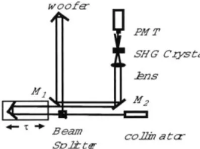
where I(t) is the intensity of the pulse under test. Physically, we split the pulse into two identical copies of itself, and then spatially overlap the two copies together inside a noncentrosymmetric X(2) crystal optimized for second harmonic generation
(SHG) (Figure 3.1). The crystal should be oriented to maximize the phase-matching woofe
SHG Czysta
NJ MI2
Beam coZZin
ata-Figure 3.1: Experimental setup for the measurement of optical pulses using
optical autocorrelation. (fig/autocorrsetup.eps)
to obtain a strong sum harmonic signal. This requirement is met by orienting the crystal such that the dispersion of the refractive index is compensated by the crystal birefringence effect.
The crystal will produce a pulse at twice the frequency of the original pulse with an intensity proportional to the product of the input intensities. This second order process is the sum harmonic generation, and is given by
p(2)(WI + w2) = 2X(2)(wi + w2)E1E2. (3.2)
In the case of an autocorrelation, Wi W2. Integrating the output of the crystal will then give us the autocorrelation of the pulse. We perform the integration by passing the sum harmonic field into a photodetector, which integrates the results and passes it
to an oscilloscope to be displayed. A rough estimate of the pulse length can be made
by observing the full width at half max (FWHM) of the autocorrelation output. This
estimate can be further refined by measuring the spectrum of the pulse and calculating the time-bandwidth product, as explained in Section 3.2. The autocorrelation is also useful in detecting the presence of distortions that would affect the intensity envelope of the pulse.
The resolution of the autocorrelator is related to both the step size of the stage as well as the bandwidth of the nonlinear crystal. The stage controls the overlap of the two pulses and the step size determines how closely spaced our measurements are. In the laboratory, our stages have step sizes of 10 p m, which corresponds to a step size of approximately 0.8 fs. This is plenty of resolution for pulses on the order of a few picoseconds. The bandwidth of the nonlinear crystal also needs to be large enough to accommodate the pulse bandwidth. If not, the pulses will be distorted as they are
passed through the crystal, and an accurate autocorrelation will not be possible.
The shortcomings of the autocorrelation are readily apparent. It is clear that any autocorrelation will result in a symmetric output regardless of the input pulse asym-metries. Furthermore, the autocorrelation will always only give information about the pulse intensity, omitting any information about pulse phase or chirp. However, more information about a pulse can be obtained when the autocorrelation is used in conjunction with spectral measurements of the pulse.
3.2
Spectral Measurements
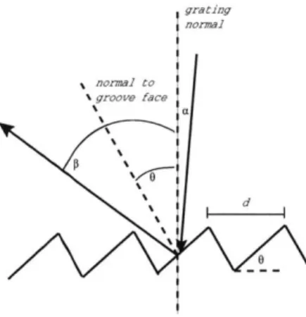
The spectrum of a pulse is easily obtained using a spectrometer. Spectrometers, monochromators, and spectrum analyzers are all based on the concept of using a grating to spatially separate the different frequency components of a pulse. A grating is a reflective piece of material which is usually scored with thin lines. When light hits these lines, it reflects off in a range of angles. At certain angles, light of a specific wavelength will interfere constructively. Other wavelengths will constructively interfere at other angles. This has the overall effect of separating the wavelengths in the incoming light.18 The general equation for a diffraction grating is
mA = d(sin a - sin 0), (3.3)
where m is the diffraction order, A is the wavelength of interest, d is the grating period, a is the angle of the incident light with respect to the grating normal, and
3 is the angle the diffracted light makes with the grating normal. Figure 3.2 is
a diagram which illustrates grating operation. The resolution of a spectrometer is determined by the amount of dispersion given by the diffraction grating. The angular dispersion measures how widely separated two different wavelengths are, and is given
by differentiating the grating equation and assuming the incident angle is fixed. We
obtain
d- =- m (3.4)
dA dcoso*
We are generally more interested in the measure of linear dispersion, which tells us how widely spaced the different wavelengths are at the focal plane of detection. The more
grating normal
% normal to
\groove face
Figure 3.2: Cross-section diagram of grating and angles associated with it. ca is the angle of incidence of the light, 0 is the blaze angle,
fi
is the angle of diffraction, and d is the grating period.19 (fig/gratingeq eps>widely spaced adjacent wavelengths are, the more easily we can distiguish between them. This gives us an idea as to the resolution of the spectrometer. To calculate the linear dispersion, we multiply the angular dispersion with the focal length of the spectrometer.
dx df3(5
dIA dA~
A spectrometer can be used in order to increase the accuracy of pulse characteri-zation measurements over those made with an autocorrelator alone. A fairly accurate estimate of the pulse length can be made by first assuming the pulse is transform lim-ited. This statement means that the Fourier transform of the real portion of the E field is the same as the Fourier transform of the complex E field of the pulse. Transform-limited also implies that no chirp exists for the pulse. In order to determine when a pulse is transform-limited, we consider the time-bandwidth product Aw/At. However,
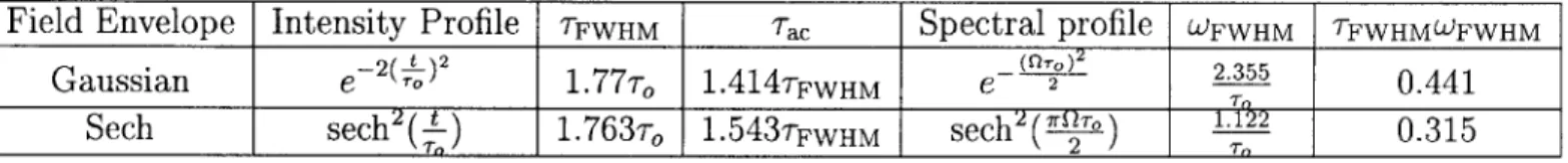
this relation is different for different pulse shapes (gaussian, sech, etc.). The tradi-tional method of determining if a pulse is transform limited is to make an estimate as to the pulse shape (gassian, sech, etc), and then to find if the time-bandwidth product is close to what it would be if it were transform-limited. If the time-bandwidth prod-uct indicates that the pulse is near transform-limited, we can assume it is transform limited. We can calculate the relation between the FWHM of an autocorrelation of a pulse and the pulse length provided the pulse is transform-limited. This also requires the assumption of a pulse shape. If the time-bandwidth product indicates that the pulse is not transform-limited, we cannot calculate the relation between the FWHM of its autocorrelation and the pulse length without knowing the extent of the chirp. As a result, non-transform-limited pulse lengths are impossible to characterize us-ing only an autocorrelator and a spectrometer. Table 3.1 shows the time-bandwidth product and the relation between the pulse length and autocorrelation FWHM for a few common pulse shapes.
Even if a spectrometer is added to the measurment, pulse characterization us-ing autocorrelation obviously requires many assumptions, which may or may not be correct. Furthermore, if the pulse is not transform-limited and has been severely distorted, no reliable way of arriving at a measurement of pulse length using the autocorrelation has been found. In order to solve all these problems, FROG was developed to characterize ultrashort pulses in the femtosecond regime.
3.3
Frequency-Resolved Optical Gating
The idea of a spectrogram has been present in acoustics for a while before being applied to the field of optical communications.2' However, the significance was not yet
Field Envelope Intensity Profile TFWHM Tac Spectral profile WFWHM TFWHMWFWHM
Gaussian e- TO 1.7 77, 1.4147FWHM e 2 0.441
Sech sech (i) 1.763T, 1.54 3TFWHM sech (r 2T) 0.315
Table 3.1: Time Bandwidth product and autocorrelation FWHM for
clear until it was shown that the spectrogram of a pulse could be used to reconstruct its intensity and phase." The spectrogram characterization technique was further refined into the current FROG method as developed by Daniel Kane, Kenneth DeLong, and Rick Trebino.8-10 Since then, many different variations in FROG measurement techniques have been developed.1'12 22 2 3
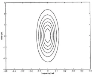
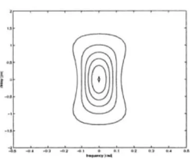
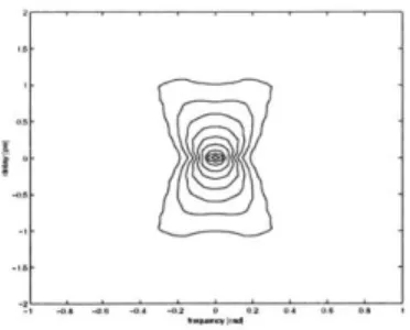
The theory behind FROG is fairly simple. In order to completely characterize the pulse under test, both time and spectral information must be measured simultane-ously. A spectrogram of the pulse plots the pulse spectral content versus the pulse temporal characteristics, as shown in Figure 3.3. To obtain a spectrogram, we first gate the original pulse E(t) with some gating function g(t). This produces one slice in time of the original pulse. We then take the spectrum of this slice in time. By varying the delay of g(t) with respect to E(t), we can obtain the spectrum of each slice of
E(t). Plotting these slices in order, we obtain a plot of both the spectral content
and temporal content of the pulse. It is clear that the gating function will determine the temporal and spatial resolution of the spectrogram, and thus the choice of g(t) is very important. Different FROG techniques choose different gating functions. The spectrogram is given by
00 2
S(w, T)= E(t)g(t - T)e-- tdt 2 (3.6)
With the spectrogram, we can completely determine the original pulse, save for an absolute phase factor. This phase factor is not of much interest to us, though it is useful in performing absolute frequency locking of ultrashort pulse lasers. In order to determine the phase of the pulse from a FROG spectrogram, an iterative algorithm is used. This process will be described in Section 3.3.3.
3.3.1
Methods for Obtaining a Trace
Many different possible methods exist to acquire a spectrogram in the laboratory. The easiest to implement is perhaps the second harmonic generation (SHG) FROG, in which the spectrogram is obtained simply by observing the spectrum of the auto-correlation of the pulse. In this case, the gating function is the pulse itself
oo 2
IFROG(W, T)
f
E(t)E(t - T)e-wdt . (3.7)This results in a spectrogram that is very sensitive, but somewhat unintuitive because the direction of time is unclear in the spectrograms from SHG FROG. This statement means that it is impossible to tell (without other measurements) whether a pulse is positively or negatively chirped due to the fact that the autocorrelation of the pulse is used. Other FROG methods include PG (polarization gate) FROG, in which the gate and pulse under test are polarized at 450 before being sent through a piece of fused silica. SD (self-diffraction) FROG has a configuration in which the gate and original pulses are sent through fused silica with the same polarization. TG (transient grating) FROG splits the original pulse in three ways, using two of the signals to induce a material grating through which the third pulse is diffracted. Finally, THG (third harmonic generation) FROG uses a glass plate to induce a surface third harmonic generation in response to the pulses. See Table 3.28 for a comparison of the different types of FROG methods.
The challenge for any FROG method we choose to implement will be to adequately resolve the pulses we are currently using in the laboratory. The system must be fairly sensitive in order to observe low energy pulses with relatively small bandwidth. (For example, if we consider a 2 ps pulse train at 10 mW with a repetition rate of 10 Gb/s,