To link to this article: DOI:10.1007/s00170-014-5652-7
http://dx.doi.org/10.1007/s00170-014-5652-7
This is an author-deposited version published in:
http://oatao.univ-toulouse.fr/
Eprints ID: 11830
To cite this version:
Msaddek, El Bechir and Bouaziz, Zoubeir and Baili, Maher and Dessein,
Gilles Influence of interpolation type in high-speed machining (HSM).
(2014) The International Journal of Advanced Manufacturing Technology,
vol. 72 (n° 1-4). pp. 289-302. ISSN 0268-3768
Open Archive Toulouse Archive Ouverte (OATAO)
OATAO is an open access repository that collects the work of Toulouse researchers and
makes it freely available over the web where possible.
Any correspondence concerning this service should be sent to the repository
administrator:
[email protected]
Influence of interpolation type in high-speed machining (HSM)
El Bechir Msaddek&Zoubeir Bouaziz&Maher Baili&
Gilles Dessein
Abstract The recourse to the high-speed machining for the manufacture of warped shapes imposes an evolution towards a very high technicality of the CAM methods and of the ma-chining operation execution. Due to its own characteristics, the high-speed machining (HSM) implies the use of new machining interpolations, in such a way that it assures the continuity of advances in the best way possible. Among these interpolations, we mention the polynomial interpolation. In this article, we propose a complete study of the interpolation type influence on the HSM machine dynamic behavior and also on the generated errors. For this, we have measured the feed rate of the cutting tool path for each type. Then, in terms of accuracy, we have measured the errors. In order to validate our approach, we have compared the simulated results to the experimental ones.
Keywords Machining . Polynomial interpolation . Modeling . Simulation . HSM
1 Introduction
For decades, a wide range of CAD/CAM systems have been used in mechanical manufacture. These systems propose
different methods of interpolation. This diversification aims to obtain the tool trajectory during the machining of complex surfaces more adapted to the CAM tolerance [1]. We distin-guish the linear interpolation, the circular interpolation, the polynomial interpolation, and the functions of compaction (Fig.1). The linear interpolation is the most frequently used, because the programmer finds it easy to use. Even if this kind of interpolation remains scarcely used, the polynomial inter-polation has the task to palliate the linear interinter-polation prob-lems. The polynomial interpolation is the generation of a tool trajectory in the form of a polynomial curve of different degrees. The spline-type interpolation (or polynomial curve bit by bit) allows the connection of a series of points of passage or of control by smoothed curves. Depending on the numerical controlled unit (NCU) and depending on the type of machine, we distinguish different types of polynomial inter-polations used in machining. These interinter-polations include Akima spline (Aspline), Bezier’s spline (Bspline), cubic spline (Cspline), and non-uniform basis rational spline (Nurbs). In polynomial interpolation, we endeavor to make the different blocks continuous in curvature so as to limit the discontinuities of speed. The functions of compaction allow the adaptation by compression in real time of the CAM trajectories. Instead of treating several small blocks, the NCU treats a more important block of displacement. These functions are based upon the compaction by polynomial in-terpolation of ten or more blocks of linear inin-terpolation G1. A block compaction must respect the programmed contour tol-erance. The more accurate the tolerance, the more impossible the block compaction becomes. Among these functions of compaction used in machining are Compon, Compcad, and Compcurv [2,3].
In high-speed machining (HSM), the feed rate becomes more and more important. However, the linear and the circular interpolations begin to present some limitations. These limi-tations occur particularly in the precision and in the time of machining because if the feed rate increases, the time neces-sary for acceleration and deceleration increases too. This has resulted in the search for a new strategy for the choice of the
E. B. Msaddek (*) Z. Bouaziz
Unit of Research of Mechanics of the Solids, Structures and Technological Development, ESSTT, University of Tunis, Tunis, Tunisia
e-mail: [email protected] Z. Bouaziz
e-mail: [email protected] M. Baili
:
G. DesseinLaboratory Production Engineering, ENIT-INPT, University of Toulouse, Tarbes, France
M. Baili
e-mail: [email protected] G. Dessein
type of tool trajectory interpolation before the program CN generation. Thus, the study shows that the interpolations alone, without considering the NCU behavior, are not in adequation with the real behavior in HSM [4]. From which, one concludes that the study of the relation between the interpolation and the HSM dynamic behavior becomes a necessity for the optimization of machining.
Recent studies have been interested in the analysis of the interpolation type influence on the machining of complex shapes in HSM. Helleno and Schutzer [1] have shown that the linear interpolation presents limitations during machining of molds in HSM and the benefits that can be found by using other types of interpolations. Guardiola et al. [5] have studied the dynamic capacity of a HSM machining center under different combinations of parameters for the machining oper-ation of complex geometries. They have determined the var-iation of the feed rate and the following error of the linear interpolation and the polynomial interpolation. Souza and Coelho [6] have proved that the type of interpolation (linear, Bspline) and the values of CAM tolerance have an important role in the machining process in terms of machining time and
surface quality. Pateloup et al. [7] have examined, at the same time, the influence of the interpolation modes, that of the curvature, and also that of the trajectory continuity on the trajectory path time of a pocket hollowing out. Tapie et al. [8] and Pateloup et al. [9] have integrated the dynamic model-ing to explain the slowdown of the HSM machine in linear and circular interpolations. Furthermore, other interpolations like Bspline were tested with the controller Siemens 840D. Prevost [10] has examined the execution errors and the ma-chining ones in the HSM manufacturing process. A compen-sation method of the contour errors for the Bspline interpola-tion has been developed. Other studies have exploited some types of polynomial interpolation to improve the machining operation. Liang et al. [11] have proposed a real-time interpo-lator with constant-length segments to improve the EDM milling of Nurbs curves. Zhao et al. [12] and Erkorkmaz et al. [13] have developed path-smoothing methods, which adopt a curvature-continuous Bspline.
In most cases, these authors have used a single type of interpolation without regard to its diversity. Up to now, few research works have been developed concerning the
(a)
(b)
(c)
Fig. 1 a Linear interpolation, b circular interpolation, and c polynomial interpolation
Fig. 2 Manufacturing process in HSM and generated errors
polynomial interpolation and its influence on the machining process in general [14], hence the interest of treating all that is related to this interpolation mode in detail. Moreover, no studies have optimized the choice of the machining interpola-tion by studying all the CAM interpolainterpola-tion types, taking account the dynamic behavior of the HSM machine, of the machining precision, and of the surface quality.
In this article, we have studied the influence of the different types of interpolation on the dynamic behavior of the HSM machine, on the machining accuracy, and on the surface state for the machining of complex shapes. Among the interpolation technologies, we have evaluated linear interpolation, polynomial interpolations (Aspline, Bspline, Cspline, and Nurbs), and functions of compaction (Compon, Compcad, and Compcurv). Our purpose is to find out the interpolation type capable of assuring a quality and a maximal productivity. For do-ing this, experimental works have been done.
2 The high-speed machining
HSM is one of the latest technologies being a part of the means provided for the enterprises to make impor-tant productivity gains. The high-speed machining of complex shapes, like molds and dies, allows the
removal of most of the materials in an object in the shortest time possible. In order to improve the manufacturing process in terms cost, time, and quality, the HSM can be a solution. From the point of view of dimensional precision, we can have a better repetition for the machining series. Besides, in HSM, we can manufacture very hard materials with longer lifetime of tools and reduced machining forces [15]. It consists not only in increasing the spindle speed but also in increas-ing the speed of a cut (more than five times superior) [8]. The real feed rate profile in HSM is variable, which indicates that several parameters must be put into evi-dence to optimize the machining of complex shapes. Hence, in order to make an optimal choice of a
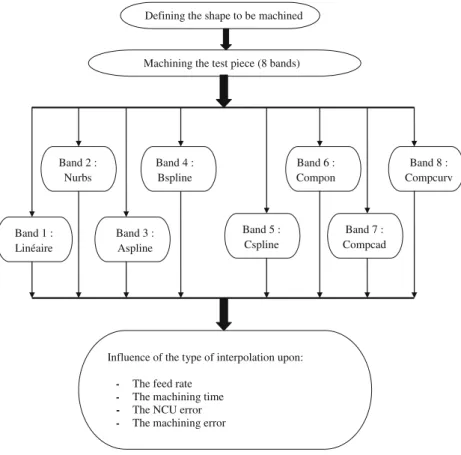
Defining the shape to be machined
Machining the test piece (8 bands)
Influence of the type of interpolation upon: - The feed rate
- The machining time
- The NCU error - The machining error Band 2 : Nurbs Band 3 : Aspline Band 1 : Linéaire Band 4 : Bspline Band 5 : Cspline Band 6 : Compon Band 7 : Compcad Band 8 : Compcurv
Fig. 3 Methodology for studying the influence of the type of interpolation
machining strategy, all we have to do is to analyze the different critical criteria [16].
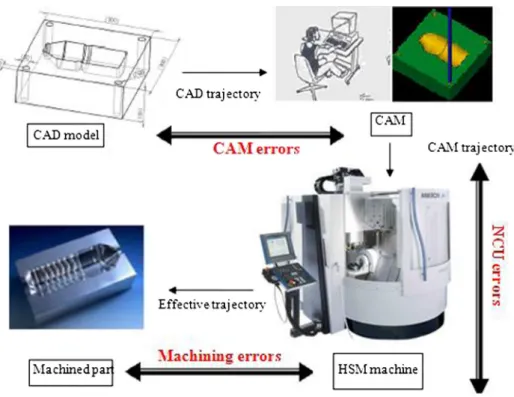
The manufacturing process in HSM has, as entry point, the CAD model from the design stage, which is the reference model constructed from a surface arrangement or geometric elements. The first step, CAM associated with the digital channel, concerns the trajectory generation or the CAM model from the CAD model. Depending on the complexity of the work surface, the differences between the nominal surface and the nominally machined surface, called CAM errors, are gen-erated. They are mainly due to numerical errors. Then, the step of execution in particular allows the generation of a relative movement of the tool relative to the workpiece. The digital part realized by the NC causes gaps called NCU errors when generating instructions of axis position. Finally, the non-ideal geometry structure of the machine, as well as associated faults (quasi-static or dynamic), is a source of errors, physical, associated with the process. Moreover, the dynamic phenom-ena associated with cutting also cause deformation of compo-nents under the effect of mechanical actions taken in. All the gaps created by the combination of these purely physical
phenomena and cutting conditions used are called machining errors [10]. Figure2shows the manufacturing process in HSM and the generated errors.
3 Influence of the type of interpolation on the warped forms in HSM
3.1 Principle and methodology
Certain types of interpolation are favorable to the machining of warped forms, whereas others are not. The linear interpo-lation is largely used in manufacture shops for the machining of several forms, but it generates remarkable limits in high-precision machining of complex-form pieces. Thus, recent researches show that there is an increase in the number of the generated CAM discretization nodes. In consequence, the length of the segments diminishes [8]. The non-utilization of “Look Ahead” (function of blocks reading anticipation) and the generation of discontinuity in tangency, or in curvature, provoke brute decelerations of the vibrations, of the shocks, and of marks on the piece. On the contrary, in the case of polynomial interpolation, if we have a polynomial of a degree superior to three, the tool acceleration becomes more contin-uous, which leads to a better trajectory quality and a surface without undesirable traces [17]. In fact, because of the lack of research in this field, we have broached the study of the influence of this type of interpolation on the HS machining of warped forms.
In order to meet the stated objectives, we have used a sample piece containing some form variations in the tool advance rate. The width of the piece allows the realization of these forms, according to the different interpolation tech-niques as shown in the organigram of Fig.3.
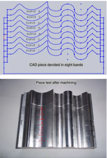
1 2 3 4 5 6 7 8
CAD piece devided in eight bands
Piece test after machining
Fig. 5 Test piece machined finish on eight bands of 10 mm by different types of interpolation
Table 1 Finish-cutting parameters Programmed speed Spindle speed Material of the part Tool CAM tolerance 4.8 m/min 24,000 rpm Aluminum Ball bur
Ø6
10μm
Table 2 Characteristics of the HSM machine Huron KX10 three axes Machine tool Characteristics
Volume of working 1,000×700×550 mm
Maximal feed rate 30 m/min (X,Y) and 18 m/min (Z) in rapid 10 m/min (X,Y,Z) work programmable Maximal acceleration 5 m/s2(X), 5 m/s2(Y), 3 m/s2(Z)
3.2 The test piece definition
The conceived test piece represents a combination of two pieces, one of them is tested by Smaoui et al. [18] and issued from [19], and the other one is tested by Helleno and Schutzer [1]. The model is made up of mono-axis, combined linear path, convex and concave circular paths, and a polynomial (spline) path, (Fig.4). This piece comprises most of the forms we can find in an industrial piece, which justifies this choice. So, the interpolations are diversified, which is interesting in order to evaluate, with precision, the machining errors and the machine dynamic behavior during the high-speed machining of a complex form.
3.3 The test piece machining
The realization of the test piece consists in machining eight bands of 10 mm each, so as to present the constant behavior zones and state the visual difference with five interpolations: G1, cubic Nurbs, of weight PW=1, and of nodal distribution (0.2, 0.2, 0.2, 0.4, 0.4, 1.5, 3.1…), Aspline, Bspline, Cspline,
and G1 with the three functions of compaction: Compon, Compcad, and Compcurv (Fig.5).
Table1presents the parameters of finish machining oper-ation of the test piece. The technical characteristics of the HSM machine Huron KX10 (three axes) are put in detail in Table 2. Besides, we have activated the anticipation (FFWON) and the smoothing (OSSE).
3.3.1 FFWON
Feed forward ON is an activation of the anticipating drive. The anticipating drive brings back to zero the distance of pursuit, which depends on the speed in a displacement with interpolation. The anticipating drive allows to increase the precision and so to improve the machining quality.
3.3.2 OSSE
This is the smoothing of the tool orientation at the beginning and at the end of the block.
Feed direction
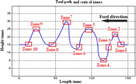
Fig. 6 Tool trajectory and critical zones
Zone 3
Zone 1
Zone 2
Zone 4
Zone 6
Zone 7
Zone 8
Zone 9
Zone 10
Zone 5
Fig. 7 Feed rate measured for the linear interpolation G1
3.4 Influence of the interpolation on the feed rate
The objective of these essays is to know the interpola-tion that urges the machine the most, since we run the risk to have vibrations and overstepping during the machining. The oscillations can lengthen the machining time as they may affect the precision and the quality of the final piece. So, each type of interpolation generates a path which is different from the other, according to the mathematical formula or the algorithm (Aspline, Cspline, etc) it describes.
In this paragraph, the experimental results of the speed profiles according to the interpolation type are presented and
examined. The measuring of the profiles is undertaken by means of a servo trace, thanks to the software SinuComNC© provided by the maker of NCU, Siemens.
Figure6presents the tool trajectory of machining and the critical zones. Figure7presents the feed rate measured for the linear interpolation G1. Figure8 presents the feed rate mea-sured for the polynomial interpolation“Nurbs”.
The feed rate in linear interpolation is variable. The speed profile oscillates following the machining path. First of all, the speed increases up to 4 m/min on the 5-mm segment. So, the programmed speed 4.8 m/min is not reached. Then, if any change of direction occurs on a critical area of strong curvature variation (Fig. 6), the
Zone 1 Zone 7
Zone 9
Zone 10 Fig. 8 Feed rate measured for the
polynomial interpolation“Nurbs”
machine decelerates to 0.2 m/min; otherwise, the ma-chine accelerates until it reaches the wanted speed. This variation is due to the dynamic behavior. The measured machining time is equal to 3.6 s with 8.213 % as percentage of the realization of the optimal feed rate.
According to Fig. 8, the feed rate of the polynomial interpolation “Nurbs” is better than that for the linear interpolation. In fact, it diminishes four times on the zones 1, 7, 9, and 10 (Fig. 6) versus ten times in linear interpolation, for the polynomial trajectory is a continu-ous curve containing discontinuities only in curvature but without discontinuities in tangency (linear interpola-tion). The modeling of the machine dynamic behavior [8] shows that the slowing down comes out of these discontinuities, where instant acceleration is variable. Hence, when the speed exceeds, the maximal accelera-tion of the axes (Table 2) imposes limited speeds. Once more, if we have a block of a small length, the time of the interpolation cycle (treatment time of the variable
CN line) limits the feed rate. Thus, the machining time measured in the polynomial interpolation is equal to 2.90 s with a percentage of the realization of the opti-mal feed rate equal to 29.063 %.
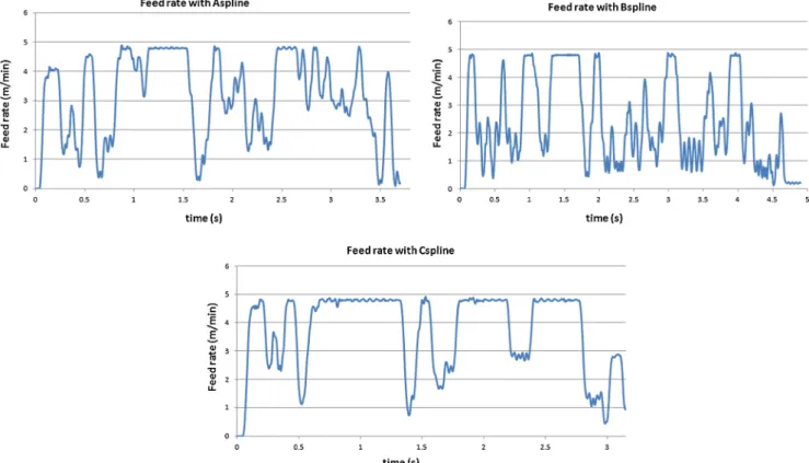
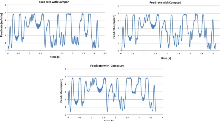
Figure 9 presents the feed rates measured in a poly-nomial interpolation: Aspline, Bspline, and Cspline. Figure 10 presents the feed rates measured for the compaction functions: Compon, Compcad, and Compcurv. Table 3presents the size of the NC file, the average speed, and the realization percentage of the programmed speed of 4.8 m/min for each interpolation.
According to Figs.9and10and to Table3, the speed of the polynomial interpolation of the Nurbs type is the most impor-tant with an average speed of 4 m/min. Whereas, the speed evolution of the polynomial interpolation of type Bspline is the most penalizing with an average speed of 2.54 m/min. When comparing the polynomial interpolation to the linear one, the first interpolation is not always favorable towards the machine dynamic behavior. The linear interpolation has an
Fig. 10 Feed rates measured for the compaction functions:“Compon”, “Compcad”, and “Compcurv”
Table 3 Average speed and the realization percentage of the programmed speed of 4.8 m/min for each interpolation
Linear Nurbs Aspline Bspline Cspline Compon Compcad Compcurv
NC file size (Ko) 209 197 202 200 200 184 200 200
Average speed (m/min) 3.219 3.997 3.142 2.542 3.764 2.825 2.915 3.068 Realization percentage ofVprog(%) 8.213 29.063 9.071 8.348 22.938 6.140 6.114 6.414
The bold values mean the favorable ones The italic values mean the non favorable ones
average feed rate more important than the polynomial inter-polation of types Aspline and Bspline. The solicitation of the machine in Bspline is due to the CAM trajectory interpolation by the controller, for the programmed positions in Bspline are not points of the curve, but only points of control of the spline. On the other side, according to the tests, it is to be noted that the CAM discretization (size of the NC file) has no influence on the speed by varying the interpolation. We find that several interpolations like the Bspline, Cspline, Compcad, and Compcurv have NC files of the same size (200 Ko) but have varied average speeds.
The “Nurbs” interpolation has the highest percentage of the Vprog realization (29 %), contrary to the compac-tion funccompac-tion “Compcad” which is 6.11 %. The “Nurbs” polynomial interpolation is very favorable towards this criterion because it is deprived of discontinuities in tangency. Thus, the compaction functions have kept a
good average speed close to 3 m/min and a low per-centage of Vprog realization, nearly 6 %, for the speed does not undergo important oscillations. In fact, the compaction of a block eliminates most of the maximum and minimum speed peaks and maintains a more impor-tant average speed. Besides, when comparing the com-paction functions to one another, the average speed of the function “Compon” is found to be the lowest, owing to the approximation by a cubic polynomial with a limited number of compacted blocks, whereas for the “Compcurv” and “Compcad” functions, the approxima-tion is carried out by a quintuple polynomial with a limited number of compacted blocks. Besides, the func-tion “Compcurv” assures the acceleration continuity to the transitions between the blocks, which explains that its speed is the most important.
3.5 The influence of the type of interpolation on the machining time
Table 4 presents the machining time by interpolation (bands of 10 mm). The average speed informs us about the machining time taken by each interpolation. Accord-ing to Table 4, we remark that the “Nurbs” polynomial interpolation is the most favorable in machining time (153.796 s). However, the “Bspline” polynomial inter-polation urges the machine more and more (252.329 s), for it provokes some strokes which have generated considerable vibrations during the machining. We do not know what causes these vibrations especially with
Table 4 Machining time according to the type of programming Interpolation CAM time (s) Machining time (s)
Linear 162 195.446 Nurbs 51 153.796 Aspline 164 186.799 Bspline 161 252.329 Cspline 162 166.115 Compon 103 187.864 Compcad 156 198.913 Compcurv 101 184.024
The bold values mean the favorable ones The italic values mean the non favorable ones
this mode of programming. A change in acceleration could result from a vibration on the machined surface, but has not been justified so far. Thus, the linear inter-polation is often more penalizing in relation to the machining time, when comparing it to the polynomial interpolation except “Bspline” and the compaction func-tion “Compcad” because its compression is realized by approximation of a “Bspline” curve.
3.6 Influence of the type of interpolation on the NCU error In order to show the influence of the type of interpo-lation on the error of the NCU, we have executed the finish of the test piece machining (Fig. 5) using the different types of interpolation. After that, we have measured the following error and the contour devia-tion for each type. In the following, and due to the considerable number of results, we are going to pres-ent the results of the most interesting interpolations (which show the best variation of the errors), linear (Nurbs) and the functions of compaction (Compon and Compcurv).
Figure 11 presents the following errors and the con-tour deviations of the linear and polynomial “Nurbs” interpolations. Figure 12 presents the following errors and the contour deviations for the “Compon” and “Compcurv” functions.
When machining the piece with different types of CAM interpolations, we remark the apparition of great specificities of each type. In the NCU, the inter-polator treats the CAM trajectory either as linear or
polynomial, generating errors of contours. Then, the set trajectories are enslaved by the buckle controllers, gen-erating following errors [10]. This objective is to know the contribution and the advantages out of the use of the polynomial interpolation. The contour and the fol-lowing error average values depending on the type of interpolation are recapitulated in Table 5.
We notice that the following error profile is identical to that of the feed rate for all the interpolations. So, the following error follows the feed rate; if the speed increases, the following error increases too and vice versa. If the programmed speed 4.8 m/min is reached, the following error attains its maximal value of 250 μm. In fact, the saturation of the acceleration on the critical zones and the limitation of the speed considered by the time IPO (NC calcula-tion of a block) promote the accuracy of the warped shape machining. Besides, the average following error of the linear interpolation is inferior to that of the polynomial interpolation. So, the linear interpolation
Fig. 12 Following errors and contour deviations for the“Compon” and “Compcurv” functions
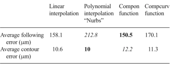
Table 5 NCU Error by interpolation Linear interpolation Polynomial interpolation “Nurbs” Compon function Compcurv function Average following error (μm) 158.1 212.8 150.5 170.1 Average contour error (μm) 10.6 10 12.2 11.3
The bold values mean the favorable ones The italic values mean the non favorable ones
imposes fewer constraints at the level of the enslave-ment position in three axes than the polynomial inter-polation “Nurbs”. We conclude that the following error follows the principle of the CAM rope error: if the trajectory generated in CAM with a specified interpola-tion is close to that of CAD, the executed trajectory is also close to that of the instruction. Moreover, we have a change of the sign in the following error, between the two interpolations. Thus, for the other interpolations (Aspline, Bspline, and Cspline), the following error varies slightly. Concerning the contour deviation, the evolution is partly constant according to the interpola-tion. We consider that the variation is negligible because of the errors of measuring.
In short, the linear interpolation and the compaction functions are the most favorable due to the following error. Hence, the NCU enslaving the system tackles the linear segments with few defects than the “Nurbs” and “Cspline” curves. This is due to the dynamics of the axes. Thus, the controller interpolator treats the polyno-mial trajectory (Nurbs and Cspline) with few defects
than the linear curve. And, this is due to the continuity of the spline curve.
3.7 The type of interpolation influence on the machining error The objective of this part is to study the influence of the type of interpolation on the machining error. We are going to use the measurement results saved by the tridimensional measuring machine (TMM) after the test piece finish machining by the different types of inter-polation. The measuring method consists of feeling the machined surface in the advance direction by saving points. The measuring is supposed to be ideal, without considering the errors of the isostatic reference piece and the imprecision envelope made up of the retiming of the points and of the diameter of the probe ball. The tested interpolations are still the same: the linear inter-polation, the polynomial interpolations (Nurbs, Aspline, Bspline, and Cspline), and the compaction functions (Compon, Compcad, and Compcurv).
0 20 40 60 80 100 120 140 160 0 5 10 15 20 25 30 35 length (mm) h e ig h t ( mm)
CAD, CAM simuted trajectories with measured trajectory of machining (Linear)
CAD trajecory CAM trajectory machining path
zoom
Fig. 13 Final machining profile (linear interpolation) with CAD and CAM profiles simulated. “trajet d’usinage” means machining path 133 134 135 136 137 138 139 140 141 15 16 17 18 19 20 21 22 length (mm) height (mm)
CAD, CAM simuted trajectories with measured trajectory of machining (Linear)
CAD trajecory CAM trajectory machining path
zoom Fig. 14 Zoomed image of the
five critical areas of machining profile in the linear interpolation. “trajet d’usinage” means machining path
The method consists in realizing a series of measures for each machining band of the test piece (Fig. 5) on a tridimensional measure machine. We consider probing each surface following a plan P in order to obtain a cloud of probed points. For each probed point, we gather the coordinates of the probe center of a diameter Ø equal to 4 mm.
Some imprecisions are generated during the measur-ing due to the slavmeasur-ing of the probe ball. Jalid et al. [20] have evaluated the uncertainty of measuring on a TMM machine. They have shown that this uncertainty is of some micrometers (2.705 μm max).
In the following, owing to the great number of results, we will mention only the results of the linear interpolation and of the polynomial interpolations: Bspline and Cspline (the clearest and the most significant). Figure 13 presents the machining profile in a linear interpolation together with the
CAD profiles (theoretical) and the profile of the simulated CAM discretization.
The trajectory profile superpositions (CAD and CAM) and machining show the influence of all the errors on the inlet trajectory (theoretical or CAD). The essays and the simulations also present the influence of the type of interpolation on the machining paths. In the linear interpolation, according to the TMM measuring, the machining path moves a few hundreds of microns away from the CAD trajectory (Fig. 14). Since the fol-lowing error does not exceed 0.25 mm, the rest of the ma-chining error is due to the elementary mama-chining cell (EMC). In general, the geometries of these zones present some diffi-culties of machining or of access to three-axis machining, because the machining is executed with the tool flank with an angle close to 90° together with other phenomena (geo-metrical defect, tool deflection, etc).
0 20 40 60 80 100 120 140 160 0 5 10 15 20 25 30 35 length (mm) height (mm)
CAD, CAM simuted trajectories with measured trajectory of machining (Bspline)
CAD trajecory Machining trajectroy CAM trajectory
zoom
Fig. 15 Final machining profile (Bspline interpolation) with CAD and CAM profiles simulated
133 134 135 136 137 138 139 140 141 14 15 16 17 18 19 20 21 22 23 length (mm) height (mm)
CAD, CAM simuted trajectories with measured trajectory of machining (Bspline)
CAD trajecory Machining trajectroy CAM trajectory
Fig. 16 Zoom image of the five critical areas of machining profile in Bspline interpolation
Figures 15 and 16 present the machining final profile (Bspline) with the simulated CAD and CAM profiles. Figure 17 presents the machining profile in Cspline i n t e r p o l a t i o n t o g e t h e r w i t h t h e C A D p r o f i l e s (theoretical) and the profile of the simulated CAM discretization.
In Bspline and Cspline interpolations, according to the TMM measuring, the machining path moves a few hundreds of microns away from the CAD trajectory, but in the critical zone (Figs. 16 and 18), it moves more than 1 mm away. The machining error is due especially to the definition of the spline trajectories. The Bspline (Bezier’s spline) is a polynomial of a cubic value or more. The programmed points do not belong to the curve but are solely points of control of the spline, i.e., the curve does not pass directly through these points, but it just tends to go towards them. The Cspline (cubic spline) is an interpolation by a cubic
polynomial. It passes exactly through the programmed points and strongly tends to oscillate between them. The polynomial interpolation of spline type presents limits in precision.
3.8 The type of interpolation influence on the surface quality After machining of the workpiece with different types of interpolation, we spent to experimentally verify the influence of each type of interpolation on the surface state. Because, it is impossible to measure the roughness on all the workpiece (size and shape), we choose an accessible zone (Fig. 19) in order to measure manually the roughness and to examine the influence of the interpolation type on the surface quality of this area. We used a roughness meter (Mahr) and a digital micro-scope (Dino-Lite) to measure the roughness and to photograph the machined surfaces.
0 20 40 60 80 100 120 140 160 0 5 10 15 20 25 30 35 length (mm) height (mm)
CAD, CAM simuted trajectories with measured trajectory of machining (Cspline)
CAD trajecory Machining trajectroy CAM trajectory
zoom
Fig. 17 Final machining profile (Cspline interpolation) with CAD and CAM profiles simulated
133 134 135 136 137 138 139 140 141 142 14 15 16 17 18 19 20 21 22 23 length (mm) height (mm)
CAD, CAM simuted trajectories with measured trajectory of machining (Cspline)
CAD trajecory Machining trajectroy CAM trajectory
Fig. 18 Zoom image of the five critical areas of machining profile in Cspline interpolation
Figure 20 shows the surface quality of a selected zone captured by a digital microscope for each interpolation. Table6 shows the value of the roughness Ra of the selected zone according to the type of interpolation.
According to the previous results, the type of interpolation affects the surface quality. The surface texture generated by the linear interpolation (G1) is worst than those of all the polynomial interpolations with Ra = 1.647 μm. So, the polynomial interpolations generate good surface quality, unlike the linear interpolation. The interpolation Nurbs presents the best roughness with Ra = 0.610 μm. On the other hand, the surface state of the interpolation Bspline is the poor between the other polynomial inter-polation with Ra = 0.845 μm. The Bspline trajectory does not pass through nodes (control points), so during machining, errors and vibrations increase which nega-tively affects the surface state. The functions of com-paction also have poor surface quality since they are derived from the linear interpolation.
We conclude that the polynomial interpolations retain bet-ter surface state than the linear inbet-terpolation and functions of compaction. The use of polynomial interpolation permits to gain in machining time and surface quality. However, these types of programming generate more machining errors.
4 Conclusion
In this article, we have been interested in the interpolation type influence on the HSM machining process, by considering some NCU and axis performances. In fact, we have measured the feed rate for the different interpolation types and also for different values of the CAM tolerance. We find that the polynomial interpolations mainly the one of Nurbs type are faster but less precise. This interpolation is the most appropri-ate for the machining of this piece type based on time and speed criteria, while the compaction functions are the most accurate. In this way, the latter have an almost similar effect as the linear interpolation.
The machining with these different types of interpo-lations also affects a criterion which is very important for complex-form machining which is the surface qual-ity. We find that the different types of polynomial Selected zone
Fig. 19 Selected zone for measuring the roughness
Table 6 Surface rough-ness depending on the type of interpolation
The bold values mean the favorable ones The italic values mean the non favorable ones
Interpolation Roughness Ra (μm) Linear 1.647 Nurbs 0.610 Aspline 0.791 Bspline 0.845 Cspline 0.647 Compon 1.254 Compcad 1.558 Compcurv 1.406
interpolations gave the best roughness, in contrast to the linear interpolation and these derivatives: the functions of compaction. Besides, this work shows surprising results which incite to consider further works of re-search, mainly about the use of “Bspline” and “Cspline” interpolations. These polynomial interpolations generate good surface quality with low precision.
According to our need (accuracy or rapidity), we choose the type of interpolation. Afterwards, we can generalize these results to any industrial piece, since our workpiece contains all possible complex forms. In fact, this work provides the prob-lematic of the warped surface pieces with the learning concerning the influence of the different types of interpolation on the HSM machining and mainly on the generated machining errors, on the machine dynamic behavior, and on the surface quality. Hence, the manufacturer has to know these results in order to choose the best type of interpolation according to his need.
References
1. Helleno AL, Schutzer K (2006) Investigation of tool path interpola-tion on the manufacturing of die and molds with HSC technology. J Mater Process Technol 179:178–184
2. Siemens (2004) Manual of programming—complementary notions: SINUMERIK 840D/840Di/810D, edition 03/2004. www. automation.siemens.com/doconweb. Accessed 26 June 2011 3. Siemens (2005) Polynomial functions and Nurbs: SINUMERIK
840D/840Di/810D, edition 2005. www.automation.siemens.com/ doconweb. Accessed 26 June 2011
4. Lavernhe S (2006) Put into account of constraints associated to MT-NC couple in generation of 5 axes trajectory in HSM. PhD thesis, the Normal School Superior of Cachan (LURPA), University of Paris
5. Guardiola A, Rodriguez Ciro A, Souza AF, Dos Santos MT (2007) Influence of tool path interpolation on cycle time and following error during high-speed milling of die and mold surfaces. Paper presented at the 6th international conference on high-speed milling, San Sebastian, Spain, 21–22 March 2007
6. Souza AF, Coelho RT (2007) Investigation of tolerances required for NC program’s generation using spline polynomial and linear inter-polation to describe a free form tool path for high speed milling. Paper presented at the 6th international conference on high-speed milling, San Sebastian, Spain, 21–22 March 2007
7. Pateloup V, Duc E, Ray P (2003) Optimization of the pockets hollowing out trajectories for the high speed milling. Paper presented at the 16th French Congress of Mechanics, Nice, pp 1–6
8. Tapie L, Mawussi KB, Anselmetti B (2006) Circular tests for HSM machine tools: bore machining application. Int J Mach Tools Manuf 47:805–819
9. Pateloup V, Duc E, Pascal R (2004) Corner optimization for pocket machining. Int J Mach Tools Manuf 44:1343–1353
10. Prevost D (2010) Modeling advanced torque machine tool/CNC in HSM to optimize the calculation of multi-axis trajectories. PhD thesis, the Normal School Superior of Cachan (LURPA), University of Paris 11. Liang S, Zhao W, Xi X (2013) Design of a real-time NURBS interpolator with constant segment length for milling EDM. Int J Adv Manuf Technol 67:427–440
12. Zhao H, Zhu L, Ding H (2013) A real-time look-ahead interpolation methodology with curvature-continuous B-spline transition scheme for CNC machining of short line segments. Int J Mach Tools Manuf 65:88–98 13. Erkorkmaz K, Yeung SH, Altintas Y (2006) Virtual CNC system: part II. High speed contouring application. Int J Mach Tools Manuf 46:1124–1138
14. Pessoles X (2010) Aid to putting-down choice in 5 axes continuous machining by the kinematic behavior modeling of the machine tools. PhD thesis, University of Toulouse, 3 Paul Sabatier (UT3 Paul Sabatier) 15. Msaddek EB, Bouaziz Z, Dessein G, Baili M (2012) Optimization of pocket machining strategy in HSM. Int J Adv Manuf Technol 62:69–81 16. Msaddek EB, Bouaziz Z, Baili M, Dessein G (2011) Modeling and simulation of high-speed milling centers dynamics. Int J Adv Manuf Technol 53:877–888
17. Duc E (1998) Machining of freeform—contribution to the improve-ment of the quality of machining paths. PhD thesis. the Normal School Superior of Cachan, France
18. Smaoui M, Bouaziz Z, Zghal A, Dessein G, Baili M (2011) Simulation of the deflected cutting tool trajectory in complex surface milling. Int J Adv Manuf Technol 56:463–474
19. Dessein G, Desforges X (2000) Path defects in high speed machining. Paper presented at the 3rd international conference on integrated design and manufacturing in mechanical engineering, Montreal, Quebec, 16–19 May 2000
20. Jalid A, Hariri S, Senelaer JP, EL Gharad A (2009) Uncertainties valuation of the measure on the tridimensional measure machine: new method of estimation of the surface parameters and associated uncertainties. 19th French congress of mechanic, Marseille, 24–28 August 2009