HAL Id: hal-01276599
https://hal.inria.fr/hal-01276599
Submitted on 19 Feb 2016
HAL is a multi-disciplinary open access
archive for the deposit and dissemination of
sci-entific research documents, whether they are
pub-lished or not. The documents may come from
teaching and research institutions in France or
abroad, or from public or private research centers.
L’archive ouverte pluridisciplinaire HAL, est
destinée au dépôt et à la diffusion de documents
scientifiques de niveau recherche, publiés ou non,
émanant des établissements d’enseignement et de
recherche français ou étrangers, des laboratoires
publics ou privés.
An automatic key discovery approach for data linking
Nathalie Pernelle, Fatiha Saïs, Danai Symeonidou
To cite this version:
Nathalie Pernelle, Fatiha Saïs, Danai Symeonidou. An automatic key discovery approach for data
linking. Journal of Web Semantics, Elsevier, 2013, 23, pp.16–30. �10.1016/j.websem.2013.07.001�.
�hal-01276599�
An Automatic Key Discovery Approach for Data Linking
Nathalie Pernelle, Fatiha Saïs, Danai Symeonidou
LRI, Paris Sud University, Bât. 650, F-91405 Orsay, FRANCE
Abstract
In the context of Linked Data, different kinds of semantic links can be established between data. However when data sources are huge, detecting such links manually is not feasible. One of the most important types of links, the identity link, expresses that different identifiers refer to the same real world entity. Some automatic data linking approaches use keys to infer identity links, nevertheless this kind of knowledge is rarely available. In this work we propose KD2R, an approach which allows the automatic discovery of composite keys in RDF data sources that may conform to different schemas. We only consider data sources for which the Unique Name Assumption is fulfilled. The obtained keys are correct with respect to the RDF data sources in which they are discovered. The proposed algorithm is scalable since it allows the key discovery without having to scan all the data. KD2R has been tested on real datasets of the international contest OAEI 2010 and on data sets available on the web of data, and has obtained promising results. Keywords: Data Linking, Identity Links, keys, Ontology
1. Introduction
Over the recent years, the number of RDF data sources available on the LOD (Linked Open Data) cloud has led to an explosive growth of the global data space (more than 31x109RDF triples as of September 20111). In this data space, establishing semantic links between data items can be really useful, since it allows crawlers, browsers and applications to combine information from different sources. These links can be set manually. However, considering the large amount of data available in the Web, some approaches propose methods that gen-erate these links between RDF data sources automati-cally. Among the different kinds of semantic links that can be established, same-as links express that different identifiers refer to the same world entity (e.g. the same restaurant, the same gene, the same person).
There are a lot of approaches that aim to detect iden-tity links between data items (see [5],[4] or [30] for a survey). In knowledge based approaches the experts de-clare knowledge that is used to infer identity links be-tween data items. Some of these approaches use rules
Email addresses: [email protected](Nathalie Pernelle), [email protected](Fatiha Saïs), [email protected] (Danai Symeonidou)
1http://www4.wiwiss.fu-berlin.de/lodcloud/state/
that specify conditions that two data items must fulfill in order to be linked. In [11,28,1] these rules are man-ually defined. In [10, 15,16] linkage rules are learnt using genetic programming techniques. [10,15] need a set of reference links to learn these rules while [16] is unsupervised and exploits assumptions on datasets and similarity functions. In [14], the authors use mathemat-ical characteristics of metric spaces to estimate the sim-ilarity between instances and filter out instance pairs.
Other approaches such as [22,8] exploit the seman-tics of the ontology such as keys, functionality of prop-erties and cardinality restrictions. Indeed, these ap-proaches give higher importance to combinations of properties that represent keys or declared as (inverse) functional during the data linking process. In LN2R data linking approach [22] a set of declared keys is ex-ploited by a logical method to generate a set of logical inference rules and by a numerical method to generate a set of similarity functions. The approach ObjectCoref [8] exploits the semantic knowledge like sameAs, (in-verse) functional properties and cardinalities to build a seed set of reference links. These links are used to learn discriminative property–value pairs.
Nevertheless, when the ontology represents many concepts and data are numerous, the linking rules or the keys that are needed for the linking step are not often
available and cannot easily be specified by a human ex-pert. Therefore, we need methods that discover them automatically from the data. Moreover, to the best of our knowledge, the approaches that focus on key dis-covery [2,25] or learning linking rules [16,10,15] in the semantic Web community use either labeled data to learn the rules [10, 15] or assume that different URIs refer to different world entities (Unique Name Assump-tion –UNA) [16,25]. If we consider the overall Linked Open Data cloud (LOD), the UNA is obviously not sat-isfied, since we can find two different URIs that refer to the same entity. However, it is not uncommon that some datasets considered separately fulfill the UNA. It can be assumed at least for all the datasets generated from re-lational databases and those created in a way to avoid duplicates like [26]. Recently, W3C has announced the recommendation R2RML2as a language for expressing
customized mappings from relational databases to RDF datasets. R2RML allows to use primary keys to gener-ate distinct URIs. This will lead to build datasets where the UNA is fulfilled.
When data are heterogeneous, the key discovery problem becomes much more complex. Hence, syntac-tic variations or errors in literal values may lead to miss keys or to discover erroneous ones. Furthermore, in the semantic Web context, RDF data may be incomplete and asserting the Closed World Assumption (CWA), i.e. what is not currently known to be true is false, as it is proposed in [2], may not be meaningful. Hence, discov-ering keys on incomplete information needs the use of heuristics to interpret the absence of information.
In this paper, we present an extension of KD2R [27], an automatic approach for key discovery in RDF data sources that conform to OWL ontologies. We aim to discover keys that are composed of several properties. Indeed, non composite keys (e.g. ISBN for books or SSN for persons) are rare in real data. Furthermore, we focus on the discovery of keys that are valid against the considered data. Unlike [2], in this work we do not aim to discover pseudo-keys, that are properties for which some instances are allowed to have the same values.
Like [2, 25], KD2R discovers keys from datasets where the UNA is fulfilled in each of its data sources. As for the Open World Assumption (OWA), KD2R may use either a pessimistic or an optimistic heuristic to in-terpret the absence of information. In [27], we have defined a first algorithm to compute keys when both heuristics can be applied. In this paper we propose a scalable algorithm which is based on the use of an opti-mistic heuristic.
2http://www.w3.org/TR/r2rml/
Unlike the approach that we have presented in [27], in case of different data sources that conform to distinct ontologies we use ontology alignment tools that create mappings between the ontology elements (see [19] for a recent survey on ontology alignment). These mappings will be used to obtain keys that are valid in all the data sources.
To avoid scanning all the data, KD2R discovers first maximal non keys (i.e., a set of properties having the same values for several instances) before inferring the keys. In addition to this, KD2R exploits key inheritance between classes in order to prune the non key search space.
The approach has been implemented and evaluated on five different datasets. To evaluate the quality of the discovered keys, they have been used in a linking process on benchmark datasets. The results that are obtained by LN2R using KD2R keys showed that the use of keys has led to infer more relevant identity links than the ones found when keys were not used. Further-more, KD2R has been applied on DBpedia data and it has shown that it can scale to millions of triples.
The remainder of this paper is organized as follows. We first describe the data and the ontology model in Section2and formalize the problem in Section3. We present the KD2R approach in Section4and the key dis-covery algorithms in Section5. Then, in section6, we present the optimistic algorithm of key discovery. After that, we present the experiment results in Section7. We conclude our presentation with an overview of related work (Section8) and concluding remarks (Section9).
2. Ontology and Data Model
We consider RDF3 data sources, each conforming
to an OWL4 ontology. The Web Ontology Language
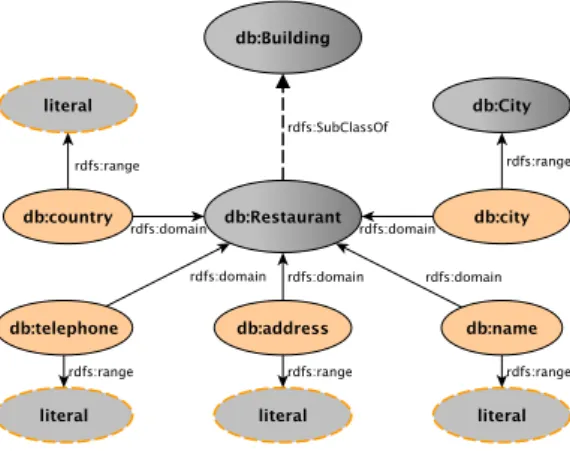
(OWL) allows to declare classes and (data or object) properties which can be organized in a hierarchy using the subsumption relation. A set of constraints can also be declared in the ontology. In Figure1, we present a part of DBpedia ontology concerning restaurants (name space db5). The class db:Restaurant is described by its name, its telephone number, its address and finally the city and the country where it is located. The class db:Restaurant is a subclass of the class db:Building.
OWL2 allows us to express keys for a given class: a key hasKey (CE(ope1, . . . , opem) (d pe1, . . . , dpen))
3www.w3.org/RDF
4http://www.w3.org/TR/owl2-overview 5http://dbpedia.org/ontology/
Figure 1: A small part of DBpedia ontology for the restaurants
states that each instance of the class expression CE6
is uniquely identified by the object property expres-sions opeiand the data property expressions d pej. This means that there is no couple of distinct instances of CE that shares values for all the object property expressions opeiand all the data property expressions d pej. An Ob-jectProperty Expression is either an ObOb-jectProperty or Inverse ObjectProperty. The only allowed data property expression is a dataTypeProperty.
For example, we can express that the property expres-sion {db:address} is a key for the class db:Restaurant using hasKey(db:Restaurant(()(db:address)).
An RDF data source contains a set of class instances described by a set of class facts and property facts. Henceforth, we will use the relational notation: C(X) is used to express that X is an instance of C and p(X, Y) expresses that the couple (X, Y) is an instance of p.
We assume that OWL entailment rules [18] are ap-plied on the RDF facts.
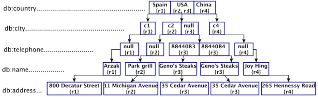
For example, the RDF source s1 contains the RDF descriptions of four db:Restaurant instances.
6We consider only the class expressions that represent OWL
classes
Source s1:
db:Restaurant(r1), db:name(r1,00Arzak00), db:city(r1, c1),
db:address(r1,00800 Decatur S treet00), db:country(r1,00S pain00),
db:Restaurant(r2), db:name(r2,00Park Grill00), db:city(r2, c2), db:address(r2,0011 North Michigan Avenue00),
db:country(r2,00US A00),
db:Restaurant(r3), db:name(r3,00Geno0s S teaks00),
db:country(r3,00US A00), db:telephone(r3,00884 − 408300),
db:telephone(r3,00884 − 408400), db:address(r3,0035 cedar Avenue00), db:Restaurant(r4), db:name(r4,00joy Hing00), db:city(r4, c4), db:address(r4,00265 Hennessy Road00), db:country(r4,00China00)
3. Problem Statement
Keys express combinations of properties that uniquely identify each instance. For this reason, keys are commonly used in data linking approaches [22,17,28] to infer identity links between instances.The keys are rarely available and not obvious to be declared by a human expert. In this paper, we focus on the automatic discovery of composite keys from data sources where information can be incomplete. We are interested in discovering keys that are valid in several data sources. A key is considered as valid in a data source if, for all pairs of distinct instances, there exists at least a value of a property expression belonging to the key that is different. However, when the UNA is not fulfilled, we cannot be sure if two instances are distinct or not. Hence, it is not obvious to distinguish the following two cases: (i) redundant property values describing data items that refer to the same real world entity and (ii) redundant property values describing data items that refer to two distinct real world entities, i.e. these values instantiate a property expression(s) that is (are) not a key.
Example: Consider an additional instance db:Restaurant(r5), in the source s1, with the same value for the property db:name(r5,00Geno0s S teaks00) as r3. If the UNA is not fulfilled, the probability for the property db:name to be a key will depend on the probability of r3 and r5 to refer to the same restaurant.
Since we are interested in the discovery of valid keys, we only consider data sources where the UNA is ful-filled.
The data sources may not be described using the same ontology. This is why we assume equivalence mappings between classes and properties that are declared or com-puted by an ontology alignment tool. If we consider that all the data sources are united in a single data source (under an integrated ontology), the UNA would be no longer guaranteed. Therefore, we tackle the problem
where the keys are first discovered in each data source and then merged according to the given mapping set.
Let s1 and s2be two RDF data sources that conform to two OWL ontologies o1, o2respectively.
We consider in each data source sithe set of instan-tiated property expressions Pei= {pei1, pei2, . . . , peiN}. Let Ci= {ci1, ci2, . . . , ciL} be set of classes of the the on-tology oi. Let M be the set of equivalence mappings between the elements (property expressions or classes) of the ontologies o1and o2. Let Pe1c(resp. Pe2c) be the set of properties of Pe1 (resp. of Pe2) such that there exists an equivalence mapping with a property of Pe2 (resp. of Pe1).
The problem of key discovery that we address in this work is defined as follows:
1. for each data source siand each class ci j∈ Ciof the ontology oi, such that it exists a mapping between a class ci j and a class cksof the other ontology ok, discover the parts of Pei that are keys in the data source si
2. find all the parts of Peic that are keys for equiva-lent classes in the two data sources s1and s2with respect to the property mappings in M.
4. KD2R: Key Discovery approach for Data Linking Given two RDF data sources and two domain ontolo-gies, KD2R aims at finding automatically keys for each instantiated class of each ontology of each considered data source. The obtained keys are then merged in or-der to find keys that are valid in all the consior-dered data sources.
In this section, we will introduce some preliminary definitions and then we will present an overview of KD2R approach.
4.1. Keys, Non Keys and Undetermined Keys
We consider that a set of property expressions is a key(c.f. definition 1) for a class if for all pairs of distinct instances of this class, there exists a property expression in this set such that all the values are distinct (objects or literal values). We consider that a set of property expressions is a non key (c.f. definition 2) for a class if there exist two distinct instances of this class that share the same values for all the property expressions of this set.
Since real RDF data sources might contain descrip-tions that are incomplete, some combinadescrip-tions of prop-erty expressions are neither keys nor non keys. More precisely, a set of property expressions is called an un-determined key(c.f. definition 3) for a class if it is not a
non key and there exist two instances of the class such that the instances share the same values for a subset of the property expressions. The remaining property ex-pressions are unknown for at least one of the two in-stances.
Distinguishing undetermined keys from keys and non keys allows us to use them in different ways. Using a pessimistic heuristic, the property for which no value is given can take all the values that appear in the data source. Therefore, the undetermined keys will not be considered as keys. Using an optimistic heuristic, the not given property values are different from all the values that appear in the data source for this property. This leads to consider the undetermined keys as keys. These undetermined keys can be validated by a human expert. Indeed, it allows a system to propose to the expert all the candidate keys that can be valid regarding to the dataset(s).
Let si be an RDF data source that conforms to an OWL ontology oiand is under the UNA.
Definition 1. – Key. A set of property expressions ksi.c = {pe1, . . . , pen} is a key for the class c in siif:
∀X ∀Y ((X , Y) ∧ c(X) ∧ c(Y)) ⇒ ∃pej(∃U ∃V pej(X, U) ∧ pej(Y, V))∧ (∀Z ∀W ¬(pej(X, Z) ∧ pej(Y, W) ∧ (Z = W))) We denote Ksi.c the set of keys of the class c w.r.t the
data source si.
Example. {db:address} ∈ Ks1.db:Restaurant since the addresses of all the restaurants appearing in the data source s1 are distinct.
A key ksi.c is minimal if it does not exist a key k
0 si.c
such that k0
si.c⊂ ksi.c.
Definition 2. – Non key. A set of property expressions nksi.c= {pe1, . . . , pen} is a non key for the class c in one
data source siif:
∃X ∃Y ∃Z1, . . . , ∃Zn(pe1(X, Z1) ∧ pe1(Y, Z1) ∧ . . . ∧ pen(X, Zn) ∧ pen(Y, Zn) ∧ (X , Y) ∧ c(X) ∧ c(Y)) We denote NKsi.cthe set of non keys of the class c w.r.t
the data source si.
Example. {db:country} ∈ NKs1.Restaurantsince there are two restaurants that are located in the same country (USA) in the data source s1.
(a) KeyFinder for one data source (b) Key merge for two data sources
Figure 2: Key Discovery for two data sources
A non key nksi.c is maximal if it does not exist a non
key nk0
s.csuch that nks.c⊂ nk0s.c.
Definition 3. – Undetermined Key. A set of property expressions uksi.c = {pe1, . . . , pen} is an undetermined
key for the class c in siif: • (i) uksi.c< N Ksi.cand
• (ii)∃X ∃Y (c(X) ∧ c(Y) ∧ (X , Y) ∧ ∀pej ((∃Z (pej(X, Z) ∧ pej(Y, Z))∨ @W (pej(X, W) ∨ @W pej(Y, W)))) We denote U Ksi.c the set of undetermined keys of the
class c w.r.t the data source s.
Example. {db:country, db:city} ∈ U Ks1.Restaurant since it is not a non key and there are two restaurants in the same country(USA) but one of them doesn’t contain any information about the city where it is located.
An undetermined key uksi.cis maximal if it does not
exist an undetermined key uk0
si.csuch that uksi.c⊂ uk
0 si.c.
4.2. KD2R overview
The most naive automatic way to discover the keys is to check all the possible combinations of property ex-pressions that refer to a class. Assume that we have a class that is described by 15 properties. In this case, the number of candidate keys is 215− 1. In order to mini-mize the number of computations, we propose a method inspired by [23] which first retrieves the set of maximal non keys (i.e. combinations of property expressions that share the same values for at least two instances) and then computes the set of minimal keys, based on the set of the discovered non keys. Indeed, to make sure that a set of property expressions is a key, we have to scan the whole set of instances of a given class. On the other hand, finding two instances that share the same values for the considered set of property expressions would suffice to be sure that this set is a non key.
In Figure2we show the main steps of the KD2R ap-proach. Our method discovers the keys for each RDF data source independently. In each data source, KD2R is applied on the classes in topologically sorted order. In this way, the keys that are discovered in the su-perclasses are exploited in the processing of their sub-classes. For a given data source siand a given class c we apply KeyFinder (Algorithm1) which aims at finding keys for the class c that are valid in the data source si.
KeyFinder starts by building a prefix tree for this class to represent its instances (see Figure2(a)). Using this representation the sets of maximal undetermined keys and maximal non keys are computed. These sets of un-determined keys and non keys, are used to derive the set of minimal keys. The obtained keys are then merged in order to compute the set of keys that are valid for both data sources (see Figure2(b)).
5. KD2R general algorithm
The main algorithm of the KD2R approach is KeyFinder (Algorithm1), which retrieves for each RDF data source, conforming to an OWL ontology, the mini-mal keys that can be added to the classes of the ontology. KeyFinder, starts by computing the topological order of the classes by exploiting the subsumption relation be-tween them.
For each class, KeyFinder builds an intermediate pre-fix tree (see Algorithm7) which is a compact represen-tation of the class instances in the data source. Then the final prefix tree (see Algorithm3) is generated in order to take into account the possible unknown prop-erty values. Using the final prefix tree the U NKFinder method is called to retrieve the maximal non keys and the maximal undetermined keys using inherited keys if there exist. Finally, KeyFinder computes the complete set of minimal keys for each class.
KeyFinder (Algorithm 1) corresponds to the pes-simistic heuristic. To consider the optimistic one, it suf-fices to call the keyDerivation (6), method using only the set of non keys NKs.c.
Algorithm 1: KeyFinder
input : s: RDF Data source, O: Ontology
output : Keys: the set of minimal keys for each class c of O
1 classList ← topologicalS ort(O);
2 while (classList , ∅) do
3 c ← getFirst(classList) //get and delete the first element;
4 tripleList ← instanceDescriptions(c); 5 if tripleList , ∅ then
6 IPT ← createIntermediatePre f ixT ree(tripleList);
7 FPT ← createFinalPre f ixT ree(IPT );
8 level ←0; U Ks.c← ∅; NKs.c← ∅; curU NKey ← ∅;
9 inheritedKeys ←
getMinimalKeys(Keys, c.superClasses);
10 U NKFinder(FPT.root, level, inheritedKeys, U Ks.c, 11 NKs.c, curUNKey);
12 keys ← keyDerivation(U Ks.c, NKs.c);
13 Ks.c← getMinimalKeys(inheritedKeys.add(keys));
14 Keys.c ← Ks.c//store the minimal keys of c;
15 return Keys
5.1. Prefix Tree creation
We now describe the creation of the prefix tree which represents the instances of a given class in one data source. We consider that the RDF descriptions of the instances are saturated using the OWL entailment rules [18].
Each level of the prefix tree corresponds to a property expression pe. Each node contains a set of cells and a variable number of cells. Each cell contains:
1. a cell value: (i) when pe is a property, the cell value is one literal value, one URI instantiating its range or a null value and (ii) in case pe is a inverse prop-erty, the cell value is one URI instantiating its do-main or an artificial null value.
2. a URI list (UL): (i) when pe is a property the URI list is the set of URIs instantiating its domain and having as range the cell value, and (ii) in case pe is an inverse property, the URI list is the set of URIs instantiating its range and having as domain the cell value.
3. a URI list (NUL): the list of URIs for which the property expression value is unknown and for which we have assigned the cell value (null or not). 4. a pointer to a single child node.
Each prefix path corresponds to the set of instance URIs that share the cell values for all the property ex-pressions involved in the path.
In order to consider the cases where property values are not given in the data source, we create first an inter-mediate prefix tree. In this interinter-mediate prefix tree, an artificial null value is created for those properties. The final prefix tree is generated by assigning all the exist-ing cell values of one node to the cell that contains the artificial null value.
5.1.1. Intermediate Prefix Tree creation
In order to create the intermediate prefix tree we use the set of all property expressions that appear at least in one instance description of the considered class. For each value of a property expression, if there is no exist-ing cell value with the same value a new cell is created and the URI list UL is initialized with the instance URI. When a property expression does not appear in the de-scription of an instance, we create or update, in the same way, a cell with an artificial null value. This intermedi-ate prefix tree creation is done by scanning the data only once.
Algorithm 2: Intermediate prefix tree creation
input : RDF DataSet s , Class c output : root of the intermediate prefix tree
1 root ←newNode();
2 Pe ← getPropertyE xpressions(c, s);
3 for each c(i) ∈ s do
4 node ← root; 5 for each pek∈ Pedo 6 if pekis inversethen 7 pek(i) ← getValues(Range); 8 else 9 pek(i) ← getValues(Domain); 10 if pek(i)= ∅ then
11 if (there is a cell cell1in node with null value)
then node.cell1.UL.add(i); 12 else cell1← newCell(); 13 node.cell1.value ←null; 14 node.cell1.UL.add(i); 15 else
16 for (each value v ∈ pek(i)) do
17 if (there exists a cell cell1with value v)then
node.cell1.UL.add(i) ; 18 else cell1← newCell(); 19 node.cell.value ← v; 20 node.cell.UL.add(i); 21 if (pekis not the last property)then
22 if cell1hasChildthen node ← cell.child.node(); 23 else node ← cell.child.newNode();
24 return root;
Example of Intermediate Prefix Tree creation. The cre-ation of the intermediate prefix tree (see Figure3) starts with the first entity which is the db:Restaurant r1. A new cell is created in the root node describing the name of the country in which the restaurant is located. The next information concerning this restaurant is the city where it is located. To store this information a new node will be created as a child node of the cell “Spain”. A new cell is created in this node to store the value c1. The process continues until all the information about an entity are represented in the tree. For each new entity, the insertion begins again from the root.
In figure3, we give the intermediate prefix tree for the class db : Restaurant instances of the RDF data source s1 described in section2.
5.1.2. Final Prefix Tree creation
We generate a final prefix tree from the intermediate prefix tree (see Algorithm3) by assigning the set of the possible values contained in the cells of one node to the artificial null value of this node, if it exists. We use the URI list NUL to store the URIs for which the property expression value was unknown. This information will
be used by UNKFinder (Algorithm 5) to distinguish non keys from undetermined keys.
Example of Final Prefix Tree creation. As we can see in Figure 3 there are two restaurants in USA: r2 and r3. The restaurant r2 is located in c2 while there is no information about the location of r2. This absence is represented by a null cell in the intermediate prefix tree (see Figure 3). Therefore, we assign the value c2 for the property db : city of r3. The URI list NUL is now {r2, r3} and r3 is stored in the list NUL (see Figure 5(b)). This assignation is performed using the mergeCells function. This process will be applied recursively to the children of this node (see Figure
5(c)) in order to: (i) merge the cells of the child nodes that contain the same value and (ii) to replace the null values by the possible ones. In figure 4, we give the final prefix tree of the RDF data described in section2.
Algorithm 3: Final prefix tree creation
input : IPT : intermediate prefix tree output : FPT : final prefix tree
1 FPT.root ← mergeCells(getCells(IPT.root)) ; 2 foreach cell c in FPT.root do
3 nodeList ← getS electedChildren(IPT.root, c.value); 4 nodeList.add(getS electedChildren(IPT.root, null)); 5 c.child ← mergeNodeOperation(nodeList); 6 return FPT ;
Algorithm 4: Merge Node Operation
input : (in) nodeList, a list of nodes to be merged output : mergedNode, the merged node and its
descendants
1 cellList ← getCells(nodeList);
2 mergedNode ← mergeCells(cellList);
3 if nodeList contains non leaf nodes then
4 foreach cell c in mergedNode do
5 childrenNodeList.add(getS electedChildren(nodeList, null)); 6 childrenNodeList.add(getS electedChildren(nodeList, c.value)); 7 c.child ←
mergeNodeOperation(childrenNodeList);
8 return mergedNode;
5.2. Undetermined and non key discovery (UNKFinder) UNKFinder algorithm aims at retrieving the maximal undetermined keys U Ks.c and the maximal non keys NKs.c from a final prefix tree(see Algorithm 3). The
Figure 3: Intermediate prefix tree for the db : Restaurant class instances
Figure 4: Final prefix tree for the db:Restaurant class instances
Figure 5: Example of merge Node Operation
traversal of the prefix tree is depth-first. This method searches the biggest combination of property expres-sions having values that are shared by more than one instance in the dataset, using a depth-first traversal of the tree. This means that this combination of property expressions represents either a non key or an undeter-mined key.
More precisely, when a leaf node is reached, if one of the cells of this leaf node contains a list of URIs (UL) with size >1, we are sure that the constructed list of property expressions (curU NKey) is either a non key
or an undetermined key . If one of the URIs of UL is obtained by a merge operation with a null value then curUNKey is an undetermined key otherwise it is a non key.
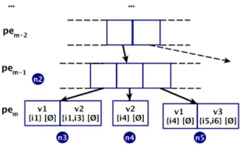
Figure 6: Example 1
In the example of Figure6, the combination of prop-erty expressions {pe1, . . . , pem} is an undetermined key. In addition to this, when the size of the union of all the URI lists UL of the leaf node is greater than 1, we
know that curU NKey that is constructed before adding the leaf level is a non key or an undetermined key (same criteria than above to distinguish them).
Figure 7: Example 2
In the example of Figure 7, in the node n2, since | {i1} ∪ {i2} |> 1, then {pe1, . . . , pem−1} is a non key or an undetermined key.
In order to generate all the possible combinations of property expressions, we need to ignore some of them (i.e., level(s) in the prefix tree). Therefore the descen-dants of the ignored level(s) have to be merged using the merge node operation (see Algorithm4).
Figure 8: Example 3
In the example of Figure 8 we illustrate how the merge node operation is used to build all the possible prefix trees corresponding to the possible combinations of property expressions. The first list of property ex-pressions {pe1, . . . , pem−1, pem} is tested successively on the leaf nodes n3, n4and n5.
Then, pem−1 is suppressed from this combination thanks to the merge node operation applied on the chil-dren of n2. The new prefix tree is shown bellow in Fig-ure9, where n6 represents the result of the merge op-eration on n3, n4 and n5. This operation is reapplied recursively on the new prefix trees obtained from the merge.
Figure 9: Example 4
To ensure the scalability of the undetermined and non key discovery, UNKFinder performs three kinds of pruning:
(A) The subsumption relation between classes is ex-ploited to prune the prefix tree traversal. Indeed, when a key is already discovered for a class using one data source, then this key is also valid for all the subclasses in this data source. Thus, parts of the prefix tree are not explored.
Example: let ks.c1 = {{pe1, pe3}, {pe2, pe4}} be the set of keys of c1. Let c2be a subclass of c1in the ontology. Let consider the prefix tree for c2showed in Figure10.
Figure 10: Example 5
When curU NKey = {pe1, pe2, pe3} the pruning is applied because curUNKey includes one of the keys of c1(i.e., {pe1, pe3}). Therefore, the subtree rooted at n3is not explored.
(B) When all the further new combinations of prop-erty expressions in a given path cannot lead to new
Algorithm 5: UNKFinder
input : (in) root: node of the prefix tree; (in) level: property expression number;
(in) inheritedKeys: keys inherited from super-classes;
(in/out) U Ks.c: set of undetermined keys ; (in/out) NKs.c: set of non keys ; (in/out) curU NKeys.c: candidate undetermined or non key
1 curU NKey.add(level) 2 if (root is a leaf) then 3 foreach cell c in root do 4 if (c.U L.size() > 1) then
5 if (one of the cells of the prefix path comes from a merge with null value (NUL.size()>1)) then U Ks.c.add(curUNKey) 6 else
7 NKs.c.add(curUNKey) 8 U Ks.c.delete(curUNKey)
9 break
10 curU NKey.remove(level)
11 if ((root has more that one cell) AND (union(getU L(root.cells))).size() > 1)) then
12 if (one of the cells of the prefix path comes from a merge with null value (NUL.size()>1)) then 13 U Ks.c.add(curUNKey)
14 else
15 NKs.c.add(curUNKey) 16 else
17 //pruning: monotonic characteristic of keys (curU NKey is a key for the current path) 18 if (U L of each cell of root contains the same URI) then
19 return
20 //pruning: monotonic characteristic of inherited keys and anti-monotonic characteristic of non keys
21 if ((a key of inheritedKeys is not included in curU NKey) AND (new maximal non keys are achievable through the current path)) then
22 foreach cell c in root do
23 //pruning: monotonic characteristic of keys 24 if (c.UL.size() >1) then
25 UNKFinder(c.getChild,level+1,inheritedKeys, U Ks.c, NKs.c)
26 curU NKey.remove(level)
27 //pruning: anti-monotonic characteristic of non keys
28 if (new maximal non keys are not achievable through the current path) then 29 return
30 childNodeList ← getChildren(root)
31 mergedT ree ← mergeNodeOperation(childNodeList)
maximal non keys then the exploration of this path stops.
Example: let NKs.c = {{pe1, pe2, pe3}} be the set of already discovered non keys. Suppose that curNKey = {pe1}. If the remaining levels of the prefix tree do only correspond to the property ex-pressions pe2 and/or pe3 then the children of the current node are not explored.
(C) The monotonic characteristic of keys, i.e. if {AB} is a key then all the supersets of {AB} are also keys. Thus, when a node describes only one in-stance we are sure that adding more property ex-pressions in the current path will not lead to a non key.
For instance, on the RDF data source s1 described in section2, we obtain the following sets of maximal un-determined keys and maximal non keys, for the class db:Restaurant:
U Ks1.db:Restaurant= {{db:telephone, db:city, db:country}} NKs1.db:Restaurant= {{db:country}}
5.2.1. Key derivation
Once the sets of maximal undetermined keys and maximal non keys are discovered from a given data source for one class, we derive the set of minimal keys. The main idea is that a key is a set of property expres-sions that is not included or is not equal to any maximal non key or undetermined key. Thus, to build all these sets of property expressions, for each maximal non key and undetermined key, we retain the property expres-sions that do not belong to this non key or undetermined key. Then, the obtained property expressions are com-bined using a cartesian product and only the minimal sets are kept.
More precisely, to derive the minimal keys Ks.c, we first compute the union of NKs.c and U Ks.c and select the maximal sets of property expressions (see Algo-rithm6). For each selected set of property expressions, we compute the complement set with respect to the whole set of instantiated property expressions. Then we apply the cartesian product on the obtained complement sets. Finally, we remove the non-minimal keys ks.cfrom the obtained multi-set Ks.c.
Example. In the db:Restaurant example we have: U Ks1.db:Restaurant= {{db:telephone,
db:city, db:country}} and
NKs1.db:Restaurant= {{db:country}}.
Algorithm 6: Key Derivation
input : U Ks.c: set of maximal undetermined keys NKs.c: set of maximal non keys output : Ks.c: set of minimal keys
1 Ks.c← ∅
2 U NKs.c← getMaximalU NKeys(U Ks.c∪ NKs.c)
3 foreach (set of property expressions unk in U NKs.c)do
4 complementS et ← complement(unk) 5 if Ks.c=∅then
6 Ks.c← complementS et
7 else
8 newS et ← ∅
9 foreach (property expression pekin complementS et)
do
10 foreach (set of property expressions ks.cin Ks.c) do
11 newS et.insert(ks.c.add(pek)) 12 newS et ← getMinimalKeys(newS et) 13 Ks.c← newS et
14 return Ks.c
The set of maximal set of property expressions is: {{db:telephone, db:city, db:country}}.
Its complement set is: {db:address},{db:name}.
Since there is only one set of property expressions, we obtain: Ks1.db:Restaurant = {{db:address}, {db:name}}.
5.2.2. Multi-source Keys
When keys are discovered from two data sources that conform to two different ontologies, we compute the keys that are valid in both data sources. The keys are expressed using the common vocabulary. First, for each data source and class we delete from Ks.c all the keys that contain property expressions that do not belong to Peic(i.e., the set of mapped properties). Then, for each pair of equivalent classes we compute the cartesian product between their set of minimal keys. Finally, we select only the minimal ones. This way we guarantee that the obtained keys are valid in both data sources. For example, consider two data sources D= {s1, s2}, if Ks1.db:Restaurant= {{db : address},
{db : name}} and
Ks2.db:Restaurant = {{db : telephone, db: city}, {db : name}}
then the multi-source keys will be:
KD:Restaurant = {{db : telephone, db : address, db : city}, {db : name}}.
6. Optimistic Algorithm for Key Discovery
When the optimistic approach is applied a more effi-cient key discovery method can be performed. Indeed, considering that each null value can be one of the al-ready existing ones, means that we have to assign all the values to each not given one. This makes the pessimistic approach not scalable when the data are very incom-plete. As we have already mentioned the pessimistic approach considers that missing values can be any of the already existing values appearing in the data. Using this approach many keys can be lost due to data incom-pleteness. For example, if we consider a dataset describ-ing 1000 people. One of the properties is mobilePhone and it is given for 999 people. Even if all the 999 val-ues of mobilePhone are pairwise distinct for each per-son, mobilePhone will not be discovered using the pes-simistic approach. Nevertheless, mobilePhone will be discovered as key using the optimistic approach.
The keys that are discovered by the optimistic ap-proach correspond to the union of the keys (see Defi-nition 1) and the undetermined keys (see DefiDefi-nition 3). The optimistic keys are defined in Definition 4, as fol-lows.
Definition 4. – Optimistic Key. A set of property ex-pressions ksi.c = {pe1, . . . , pen} is an optimistic key for
the class c in siif:
∀X ∀Y ((X , Y) ∧ c(X) ∧ c(Y)) ⇒ (∀Z ∀W ¬(pej(X, Z) ∧ pej(Y, W) ∧ (Z= W))) We denote Ksi.cthe set of optimistic keys of the class c
w.r.t the data source si.
Using the optimistic approach, there is no more need to build the intermediate prefix tree (see Algorithm 2). Indeed, using Algorithm 7, we can build directly the final prefix tree, since no null values have to be merged.
7. Experiments
In this section we present the results of the exper-iments obtained from several datasets. First, we give the obtained keys from each dataset. For some of them we give the obtained results using both the pessimistic and the optimistic approaches. Then, in section 7.2
the scalability of our method (optimistic heuristic) is demonstrated using two datasets extracted from DB-pedia that consist of millions of triples. The evalua-tion of the quality of the discovered keys is performed using a data linking tool and we have measured the
Algorithm 7: Final Optimistic prefix tree creation
input : RDF DataSet s , Class c output : root of the intermediate prefix tree
1 root ←newNode();
2 Pe ← getPropertyE xpressions(c, s);
3 for each c(i) ∈ s do
4 node ← root; 5 for each pek∈ Pedo 6 if pekis inversethen 7 pek(i) ← getValues(Range); 8 else 9 pek(i) ← getValues(Domain); 10 for (each value v ∈ pek(i)) do
11 if (there exists a cell cell1with value v)then
node.cell1.UL.add(i) ; 12 else cell1← newCell(); 13 node.cell.value ← v; 14 node.cell.UL.add(i); 15 if (pekis not the last property)then
16 if cell1hasChildthen node ← cell.child.node(); 17 else node ← cell.child.newNode();
18 return root;
well known recall, precision and F-Measure. The ob-tained results are presented in two parts: (i) in subsec-tion7.3.1we give the obtained recall, precision and F-Measure, on one dataset, when the keys are applied us-ing equality between values (instead of usus-ing similar-ity scores) and when the linking decisions are not prop-agated (e.g. “same restaurants then, same addresses, then same cities, then, ...”); and (ii) in section7.3.2we present the obtained recall, precision and F-measure, on the other datasets, when the keys are applied all together using similarity scores between values and where the linking decisions are propagated thanks to LN2R tool (see section7.3.2).
7.1. Evaluation of key discovery
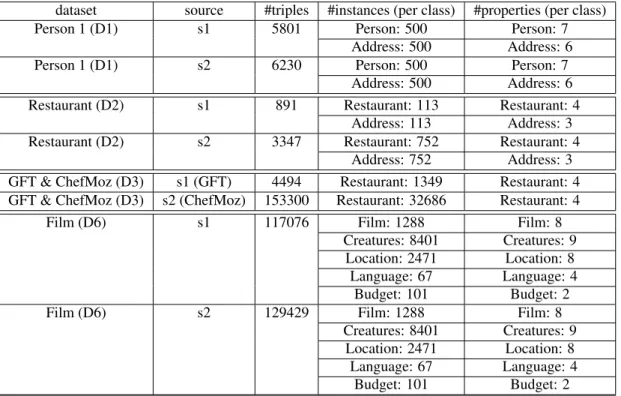
We have tested KD2R on six RDF datasets7. The
two first datasets have been used in the OAEI–Ontology Alignment Evaluation Initiative 20108, in the Instance Matching track. The three following datasets have been collected from the Web of data. The last dataset has been taken from the OAEI–Ontology Alignment Evalu-ation Initiative 20129. Each dataset contains two RDF data sources and two OWL ontologies. UNA is declared for each RDF data source of the six datasets. For each dataset, we discovered the keys using KD2R. Table 1
7http://www.lri.fr/~sais/KD2R-DataSets 8http://oaei.ontologymatching.org/2010/ 9http://oaei.ontologymatching.org/2012/
displays some statistics of the used datasets: the num-ber of triples, the numnum-ber of instances per class and the number of properties per class.
In the following, we describe each dataset and present the set of keys that are discovered by KD2R.
7.1.1. KD2R results on OAEI 2010 datasets
The first dataset D1 consists of 2000 instances of the classes Person and Address (see Table1). In the Ontol-ogy:
• a Person instance is described by the data type properties: givenName, state, surname, dateO f Birth, socS ecurityId, phoneNumber, age and the object property hasAddress.
• an Address instance is described by the data type properties: street, houseNumber, postCode, isInS uburb10and the object property hasAddress.
Both RDF data sources of the dataset D1 contain 500 instances of the class Person and 500 instances of Address.
KD2R has discovered the four following keys for the classes Person and Address in the dataset D1, using the pessimistic heuristic:
KD1.Person= {{socS ecurityId}, {hasAddress}}
KD1.Address= {{isInS uburb, postcode, houseNumber}, {inverse(hasAddress)}}.
Applying the optimistic heuristic, KD2R has dis-covered the thirteen following keys for the Person and Addressclasses in the same dataset:
KD1.Person= {{socS ecurityId}, {hasPhone} {hasAddress}, {dateO f Birth, givenName}, {dateO f Birth, age},
{surname, dateO f Birth}, {surname, givenName}} KD1.Address= {{street, houseNumber}, {street, isInSub-urb}, {houseNumber, isInS ubisInSub-urb},{postCode, isInS ubisInSub-urb}, {street, postCode}, {inverse(hasAddress)}}.
In optimistic heuristic, all the undetermined keys are considered as keys. In the Person dataset D1, there are a lot of not instantiated properties. Thus, we have obtained a lot of undetermined keys. This has led to a set of keys that is bigger than the one obtained using
10in the ontology of the second data source isInS uburb is declared
as an object property. Since, it was the unique difference between the two ontologies, we have chosen to rewrite the second data source using the first ontology. An analogous processing has been performed on the second dataset.
the pessimistic heuristic.
The second dataset D2 describes 1730 instances of Restaurantand Address classes (see Table1). It corre-sponds to the first version of the OAEI 2010 restaurant dataset that contains bugs. In the provided ontology we have:
• a Restaurant instance is described using the datatype properties properties name, phoneNumber, hasCategory and the object property hasAddress.
• an Address instance is described using the datatype properties street, city and the object prop-erty hasAddress.
The first RDF data source s1 describes 113 Address instances and 113 Restaurant instances. The second RDF data source s2 describes 752 Restaurant instances and 752 Address instances.
The five keys that are obtained for Restaurant and Addressclasses in the dataset D2, under the pessimistic heuristic, are as follows:
KD2.Restaurant= {{phoneNumber, name}, {phoneNumber, hasCategory}, {name, hasCategory}, {hasAddress}} KD2.Address= {{inverse(hasAddress)}}.
Since D2 does not contain any undetermined keys, the obtained results are the same for both the optimistic and pessimistic heuristic (see section4.1).
7.1.2. KD2R results on GFT-ChefMoz dataset
The GFT-ChefMoz dataset is composed of two RDF data sources and two OWL ontologies. The first data source has been extracted from the ChefMoz repository published on the Linked Open Data Cloud (LOD). The second data source was obtained from Google Fusion tables service [7], by [20]. In order to enforce the UNA in the ChefMoz dataset we used the linking tool LN2R without keys (see Section7.3.2). The results have been manually validated and the duplicates have been sup-pressed.
The GFT data source s1, collected from the LOD, contains 1575 instances of the class Restaurant (see1). In the ontology a restaurant is described by the data type properties: title, address, cuisine, city.
The ChefMoz data source s2 describes 32586 instances of the class Restaurant (see Table 1). In this ontology, restaurants are described using more properties than in ontology of the data source s1.
dataset source #triples #instances (per class) #properties (per class)
Person 1 (D1) s1 5801 Person: 500 Person: 7
Address: 500 Address: 6
Person 1 (D1) s2 6230 Person: 500 Person: 7
Address: 500 Address: 6 Restaurant (D2) s1 891 Restaurant: 113 Restaurant: 4
Address: 113 Address: 3 Restaurant (D2) s2 3347 Restaurant: 752 Restaurant: 4
Address: 752 Address: 3 GFT & ChefMoz (D3) s1 (GFT) 4494 Restaurant: 1349 Restaurant: 4 GFT & ChefMoz (D3) s2 (ChefMoz) 153300 Restaurant: 32686 Restaurant: 4
Film (D6) s1 117076 Film: 1288 Film: 8
Creatures: 8401 Creatures: 9 Location: 2471 Location: 8
Language: 67 Language: 4 Budget: 101 Budget: 2
Film (D6) s2 129429 Film: 1288 Film: 8
Creatures: 8401 Creatures: 9 Location: 2471 Location: 8
Language: 67 Language: 4 Budget: 101 Budget: 2
Table 1: Statistics on OAEI 2010 and GFT & ChefMoz datasets
Equivalence mappings have been declared between the four properties of GFT (s1) and the properties of ChefMoz (s2).
KD2R has discovered the following keys for the class Restaurantin the data source s1, using the pessimistic heuristic:
Ks1.Restaurant= {{address},{city, title}}
The key that is obtained for Restaurant in the data source s2 is the following composite key, using the pessimistic heuristic:
Ks2.Restaurant= {{title, address}}
After the merge, the obtained multi-source key is: KD3.Restaurant= {{title, address}}
Using the optimistic heuristic, the keys obtained on each data source are different but the key obtained af-ter their merge is equal to the one obtained using pes-simistic heuristic.
7.1.3. KD2R results on DBpedia dataset
In order to show the scalability of our method, we have applied KD2R on two datasets extracted from
DB-pedia11: the first dataset contains descriptions of
per-sons and the second one of natural places (see table2). One of the characteristics of DBpedia is that the UNA is not fulfilled. All the keys that can be discovered on such a dataset would still remain valid even if the dupli-cates are removed. However, some of the possible min-imal keys can be lost. In the worst case scenario, two duplicates are represented by the same property values. Hence, no keys can be found using these properties. In DBpedia, we have observed that some people are rep-resented several times using distinct URIs, but in differ-ent contexts (e.g. one soccer-player is represdiffer-ented using several URIs, but for each URI the description concerns its transfer into an new club). Therefore, in such cases keys can be discovered.
On small data sources such as OAEI data sources or GFT (less than 10 000 triples), KD2R can be applied us-ing the pessimistic or the optimistic heuristic. Neverthe-less, on large datasets such as DBpedia persons (more than 5.6 millions of triples) or DBpedia natural places (more than 1.6 millions of triples), the pessimistic ap-proach cannot by used. Indeed, such datasets contain a lot of properties that are rarely instantiated which leads to a final prefix tree that contains too many nodes (i.e.
assignation of all the possible values to the artificial “null” values in the prefix tree). Hence, in such cases only the optimistic heuristic can be applied. Moreover, in our experiments we have considered only the prop-erties that are instantiated for at least T distinct Person and NaturalPlace instances.
The first dataset contains 763644 instances of the class Person which corresponds to 5639680 RDF triples. The second dataset contains 49887 instances of the class NaturalPlace, or 1604347 RDF triples. To show how the inherited keys are exploited, KD2R has been applied on the class NaturalPlace, its subclass BodyO f Water and on the class Lake which is a sub-class of the sub-class BodyO f Water.
For the class Person of D4, when T is equal to 20%, the set of obtained keys is as fol-lows: KD4.Person = {{squadnumber, birthplace}, {squadnumber, birthdate}, {currentmember, birthplace}, {currentmember, name}, {squadnumber, name}, {currentmember, birthdate}}
When T is equal to 10%, KD2R obtains 17 addition-nal composite keys, such as {name, position, deathdate} and {name, occupation, birthdate, activeyearstartyear, birthplace}}
For the class NaturalPlace of D5, when T is equal to 20%, the set of obtained keys is:
KD5.NaturalPlace = {{name, district, elevation}, {sourcecountry, location}, {country, district, long}, {district, sourcecountry, elevation}, {sourcecountry, long}, {district, location}, {name, lat, district}, {country,locatedinarea}, {lat, district, elevation}, {lat, sourcecountry}, {location, locatedinarea}, {sourcecountry, locatedinarea}, {district,locatedinarea}, {name, district, point}, {country, lat, district}, {name, district, long}, {district, elevation, long}, {country, sourcecountry, elevation}, {country, district, point}, {district, point, elevation}, {sourcecountry, point}}
For the 33993 instances of the class BodyO f Water, we have found 13 keys, four of them are subsets of some minimal keys that are inherited from NaturalPlace like {lat, district}. The other minimal keys belong to the set of minimal keys inherited from NaturalPlace.
For the 9438 instances of the class Lake, we have found 7 minimal keys, three of them are subsets of some minimal keys that are inherited from BodyO f Water like {sourceCountry}. The other minimal keys belong to the set of minimal keys inherited from BodyO f Water.
7.1.4. KD2R results on IIMB dataset
The last dataset used in the experiments is the IIMB dataset (ISLab Instance Matching Benchmark), D6. This benchmark is used in the instance matching track of the Ontology Alignment Evaluation Initiative (OAEI 2011 & 2012). An initial dataset that describes movies (films, actors, directors, etc.) was extracted from the web (file 0). The classes contained in this dataset ex-cept for movies, are creatures, languages, budgets and finally locations.
Various kinds of transformations, including value transformations, structural and logical transformations, were applied to this initial dataset to generate a set of 80 different test cases. For each test case, the reference alignments are given (i.e. sameAs links between indi-viduals of the generated test case and the ones of the initial dataset). We evaluate the keys here using the first test case (file 1) in which the modifications only concern data property values (typographical errors, lexical vari-ations). Each of the two files contains 1228 descriptions of pairwise distinct film instances, 8401 descriptions of creatures, 2471 descriptions of locations, 67 descrip-tions of languages and finally 101 different descripdescrip-tions of budgets concerning the movies.
In this dataset we present only the results of the op-timistic heuristic, since the pessimistic does not scale. The number of keys discovered in each of the two files of this dataset exceeds the 30. Thus, we chose to not present them one by one but to focus on the results of linking.
For example, two of the keys found for the class Film are the following the following two keys: { f ilmedIn, directedBy, name}, {estimatedBudgetU sed}.
7.2. Scalability Evaluation
The complexity of the prefix tree exploration is ponential in terms of the number of the property ex-pression values. In order to test the scalability of our method we have checked experimentally on the seven data sources the benefits of the different kinds of prun-ing that are used durprun-ing the prefix tree exploration. More specifically, as it is already mentioned, the prun-ing that is used in KD2R can be grouped in three cate-gories:
1. Key Inheritance (see section 5.2 (A))
2. NonKey Antimonotonicity (see section 5.2 (B)) 3. Key Mononotonicity (see section 5.2 (C))
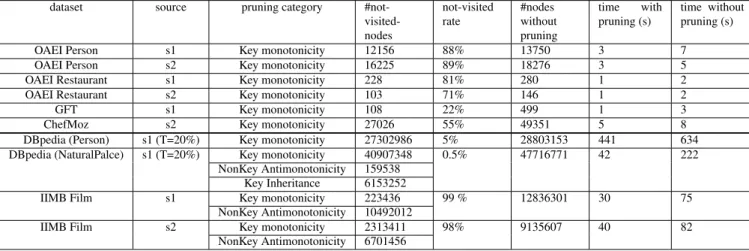
In tables 3 and 4, we give the results of KD2R in terms of runtime and search space pruning for every data source. The given results correspond to the sum
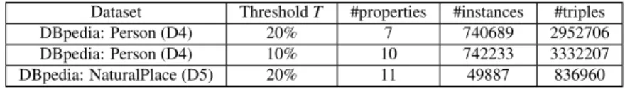
Dataset Threshold T #properties #instances #triples DBpedia: Person (D4) 20% 7 740689 2952706 DBpedia: Person (D4) 10% 10 742233 3332207 DBpedia: NaturalPlace (D5) 20% 11 49887 836960
Table 2: DBpedia dataset description
of those obtained for each class in the dataset. For ex-ample, for the data source s1, the results correspond to the results obtained for the classes Person and Address. The pruning techniques enable KD2R to be more ef-ficient and scalable in big datasets. Tables3and4show that on the five smallest data sources, the execution times of keyFinder (using pessimistic or optimistic) is less than 8 seconds. For the two DBpedia data sources, the execution times is less than 441 seconds. Thanks to the different kinds of pruning, less than 50% of the nodes of the prefix tree are explored for all datasets. Furthermore, we can notice that the more the triples are numerous the more the pruning is efficient. It should be also mentioned that for the instances of the class DB-pedia Person, less than 5% of the nodes are explored, and for the class DBpedia NaturalPlace, less than 0.5% of the nodes are explored.The dataset D5, is the only one in the experiments that contain sumbsumption re-lations between the classes. This experiment has been executed to show the importance of the Key inheritance pruning. 13% of the all the prunings that takes place in this dataset are obtained thanks to the Key Inheritance (4).
Nevertheless, even if the pruning clearly improves the execution time, the bottleneck of the approach is the computation of the minimal keys from the set of maxi-mal non keys and undetermined keys. Indeed, the com-plexity of this step is quadratic in terms of the number of non keys when the number of keys is linear with respect to the number of non keys and undermined keys. 7.3. Evaluation of the key quality
In this section we first present the results, on the IIMB dataset, of the quality evaluation results of the discov-ered keys using a linking tool without using similarity scores and without propagation. Then we give, for all the other datasets, the linking results using LN2R link-ing tool where similarity scores and decision propaga-tion are used.
7.3.1. Key quality without similarity scores and without propagation
By using a data linking tool where equality is used to compare values and where no propagation between
linking decisions is used, we have computed the recall, the precision and the F-measure obtained on a part of the IIMB dataset.
Due to the data heterogeneity of the IIMB dataset, we have obtained a low value for the recall (5.03%). Discovering keys that are valid for both datasets allows to guarantee a very high value for the precision. This is shown by the obtained precision which is of 100%. This leads to an F-Measure of about 10%. These re-sults show that the obtained keys has a good quality in terms of correctness. However, due to the heterogeneity of the data and to the fact that decision propagation is not considered the recall is very low. Hence, in order to ensure the good quality results, in terms of recall and precision, more complex linking tools that take similar-ity measures into account, appear to be necessary to be used.
7.3.2. Key quality by using similarity scores and deci-sion propagation
To evaluate the quality of the obtained keys, using a more complex way, we have used an existing data link-ing tool to show the benefits of uslink-ing discovered keys in the data linking process. More precisely, we have com-pared the results that are obtained by the linking tool when the keys that are discovered by KD2R are used and when no keys are not available.
Brief presentation of N2R. N2R is a knowledge based approach which exploits the keys that are declared in the ontology to infer identity links (reconciliation deci-sions) between class instances.
It exploits keys in order to generate a function that computes similarity scores for pairs of instances. This numerical approach is based on equations that model the influence between similarities. In the equations, each variable represents the (unknown) similarity between two instances while the similarities between values of data properties are constants (obtained using standard similarity measures on strings or on sets of strings). Fur-thermore, ontology and data knowledge (disjunction, UNA) is exploited by N2R in a filtering step to reduce the number of reference pairs that are considered in the equation system.
dataset source pruning category #not- visited-nodes not-visited rate #nodes without pruning time with pruning (s) time without pruning (s) OAEI Person s1 Key monotonicity 764478 60% 1252994 4 8 OAEI Person s2 Key monotonicity 1679956 75% 2234738 8 10
OAEI Restaurant s1 Key monotonicity 228 81% 280 1 2
OAEI Restaurant s2 Key monotonicity 103 71% 146 1 2
GFT s1 Key monotonicity 84 10% 827 1 3
ChefMoz s2 Key monotonicity 71754 55% 129569 570 625
Table 3: Pessimistic heuristic: search space pruning and runtime results
dataset source pruning category #not- visited-nodes not-visited rate #nodes without pruning time with pruning (s) time without pruning (s)
OAEI Person s1 Key monotonicity 12156 88% 13750 3 7
OAEI Person s2 Key monotonicity 16225 89% 18276 3 5
OAEI Restaurant s1 Key monotonicity 228 81% 280 1 2
OAEI Restaurant s2 Key monotonicity 103 71% 146 1 2
GFT s1 Key monotonicity 108 22% 499 1 3
ChefMoz s2 Key monotonicity 27026 55% 49351 5 8
DBpedia (Person) s1 (T=20%) Key monotonicity 27302986 5% 28803153 441 634 DBpedia (NaturalPalce) s1 (T=20%) Key monotonicity 40907348 0.5% 47716771 42 222
NonKey Antimonotonicity 159538 Key Inheritance 6153252
IIMB Film s1 Key monotonicity 223436 99 % 12836301 30 75
NonKey Antimonotonicity 10492012
IIMB Film s2 Key monotonicity 2313411 98% 9135607 40 82
NonKey Antimonotonicity 6701456
More precisely, for each reference pair, the similar-ity score is modeled by a variable xiand the way it de-pends on other similarity scores is modeled by an equa-tion: xi = fi(X), where i ∈ [1..n] and n is the num-ber of reference pairs for which we apply N2R, and X = (x1, x2, . . . , xn) is the set of their corresponding variables. Each equation xi= fi(X) is of the form:
fi(X)= max( fi−d f(X), fi−nd f(X))
The function fi−d f(X) is the maximum of the similar-ity scores obtained for the instances of the data proper-ties and the object properproper-ties that belong to a key de-scribing the i-th reference pair. In case of a combined key we compute first the average of the similarity scores of the property instances involved in that combined key. The maximum function allows to propagate the similar-ity scores of the values and the instances having a strong impact. The function fi−nd f(X) is defined by a weighted average of the similarity scores of the literal value pairs (and sets) and the instance pairs (and sets) of data prop-erties and object propprop-erties describing the i-th instance pair and not belonging to a key. See [22] for the de-tailed definition of fi−d f(X) and fi−nd f(X). Solving this equation system is done by an iterative method inspired by the Jacobi method [6], which is fast converging on linear equation systems.
The instance pairs for which the similarity is greater than a given threshold T Rec are reconciled, i.e, an iden-tity link is created between the two instances.
We have compared the obtained results with the available gold-standard using the following standard measures: precision, recall and F-measure. Then, we have compared these results to those that are obtained by N2R: (i) when no keys are declared in the ontology and (ii) when expert keys manually defined for the OAEI’10 contest are declared in the ontology.
Obtained results on OAEI 2010 datasets. Tables5and
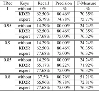
6show the results obtained by N2R in terms of recall, precision and F-measure when: (i) no keys are used, (ii) all KD2R keys are used and (iii) keys defined by experts are used [21]. Since the domains concerning persons and restaurants are rather common, the expert keys have been declared manually by one of the participants of the OAEI contest 2010, for LN2R tool. If several experts are involved, a kappa coefficient [3] can be computed to measure their agreement. Since D1 contains not in-stantiated properties, both the optimistic and pessimistic heuristic have been performed. In Table5 we define as KD2R-O the results obtained using keys discovered
with the optimistic heuristic and KD2R-P the results ob-tained using key discovered with the pessimistic heuris-tic. It should be mentioned that for the datasets D2 and D3 the results given for KD2R are both the results of KD2R-O and KD2R-P, since there are no undeter-mined keys. We show the results when the threshold T Rec varies from 1 to 0.8. Since the F-measure ex-presses the trade-off between the recall and the preci-sion, we first discuss the obtained results according to this measure. Across all datasets and values of T Rec, the F-measure obtained using KD2R keys is greater than the F-Measure obtained when keys are not available. We can notice that, the results obtained for the Person dataset (D1) are better when we use keys obtained by either KD2R-O or KD2R-P than when the keys are not used. When the threshold is bigger than 0.95 the F-Measure of LN2R using KD2R-O keys is 100%. This is an example that shows that the results using keys found with the optimistic heuristic can be better than the ones found with the pessimistic heuristic. In the restaurant dataset (D2), when T Rec ≥ 0.9, the F-measure is al-most three times higher than the F-measure obtained when keys are not declared. This big difference is due to the fact that the recall is much higher when KD2R keys are added. Indeed, even when some property values are syntactically different, it suffices that it exists one key for which the property values are similar, to infer any identity link. For example, when T Rec = 1, the KD2R recall is 95% for the persons dataset while without the keys the recall is 0%. Hence, the more numerous the keys are, the more identity links can be inferred.
Furthermore, our results are very close to the ones ob-tained using expert keys. For both datasets, the largest difference between KD2R F-measure and the expert’s one is 6%. We should also mention that KD2R preci-sion is always higher than the expert precipreci-sion. Indeed, some expert keys are not verified in the dataset. For example, while the expert has declared phoneNumber as a key for the Restaurant class,in this dataset some restaurants share the same phone number, i.e, they are managed by the same organization.
These results show that the data linking results are significantly improved, especially in terms of recall, when we compare them to results that can be obtained when the keys are not defined.
In table 7 we give a comparison between the re-sults obtained by LN2R using KD2R keys with other tools that have used the Person-Restaurant (PR) dataset of OAEI 2010–Instance Matching track. We can no-tice that the obtained results in terms of F-measure are comparable to those obtained by semi-supervised ap-proaches like ObjectCoref [8]. It is nevertheless less
ef-TRec Keys Recall Precision F-Measure 1 without 0% - % - % KD2R-O 100% 100% 100% KD2R-P 95.00% 100% 97.44% expert 98.40% 100% 99.19% 0.95 without 61.20% 100% 75.93% KD2R-O 100% 100% 100% KD2R-P 95.00% 100% 97.44% expert 98.60% 100% 99.30% 0.9 without 64.2% 100% 78.20% KD2R-O 100% 98.04% 99.01% KD2R-P 95.00% 100% 97.44% expert 98.60% 100% 99.30% 0.85 without 65.20% 100% 78.93% KD2R-O 100% 81.30% 89.68% KD2R-P 99.80% 100% 99.90% expert 99.80% 100% 99.90% 0.8 without 90.20% 100% 94.85% KD2R-O 100% 35.71% 52.63% KD2R-P 99.80% 100% 99.90% expert 100% 100% 100%
Table 5: Recall, Precision and F-measure for D1
TRec Keys Recall Precision F-Measure
1 without 0% - % - % KD2R 62.50% 80.46% 70.35% expert 76.79% 74.78% 75.77% 0.95 without 14.29% 80.00% 24.24% KD2R 62.50% 80.46% 70.35% expert 77.68% 75.00% 76.32% 0.9 without 14.29% 80.00% 24.24% KD2R 62.50% 80.46% 70.35% expert 77.68% 75.00% 76.32% 0.85 without 14.29% 80.00% 24.24% KD2R 65.17% 80.22% 71.92% expert 77.68% 75.00% 76.32% 0.8 without 37.5% 80.76% 51.21% KD2R 66.96% 79.78% 72.81% expert 77.68% 75.00% 76.32%
Table 6: Recall, Precision and F-measure for D2
ficient than approaches that learn linkage rules that are specific to the dataset like KoFuss+GA.
Obtained results for GFT-ChefMoz dataset. Table 8
demonstrates the results obtained by N2R in terms of recall, precision and F-measure when: (i) no keys are used and (ii) KD2R keys are used. We show the
re-TRec Keys Recall Precision F-Measure 1 without 45.67% 100% 62.71% KD2R 60.49% 100% 75.38% 0.95 without 50.61% 100% 67.21% KD2R 60.49% 100% 75.38% 0.9 without 50.61% 100% 67.21% KD2R 60.49% 100% 75.38% 0.85 without 50.61% 100% 67.21% KD2R 60.49% 100% 75.38% 0.8 without 54.32% 100% 70.39% KD2R 60.49% 100% 75.38% 0.75 without 54.32% 100% 70.39% KD2R 60.49% 100% 75.38% 0.7 without 60.49% 100% 75.38% KD2R 61.72% 100% 76.33%
Table 8: Recall, Precision and F-measure for D3
sults when the threshold T Rec takes values in the inter-val [0.7..1]. For both datasets and for every T Rec inter-value, the F-measure found using KD2R keys is greater than the F-Measure when keys are missing.
This difference is due to the fact that the recall is al-ways higher when KD2R keys are added. Indeed, even when some property values are syntactically different, it suffices that it exists one key for which the property val-ues are similar, to infer the reconciliation. For example, when T Rec= 1, the KD2R recall is 60% for the persons dataset while without the keys the recall is 45%. Hence, the more numerous the keys are, the more reconciliation decisions can be inferred.
As in D1 and D2, the above results show that the data linking results are significantly improved, in particular in terms of recall, when we compare them to results obtained when the keys are not defined.
8. Related Work
The problem of key discovery in RDF datasets in the setting of the semantic web is similar to the key dis-covery problem in relational databases. Nevertheless, in database area the approaches do not consider the semantics defined in the ontology (e.g. the subsumption relation that can be defined between classes). Besides, in the relational context, the key discovery problem is a sub-problem of Functional Dependencies (FDs)
Dataset LN2R+KD2R-P LN2R+KD2R-O ASMOV LN2R CODI ObjectCoref RIMOM KnoFuss+GA
Person 1 0.99 1.00 1.00 1.00 0.91 1.00 1.00 1.00
Restaurant 0.728 – 0.70 0.75 0.72 0.73 0.81 0.78
Table 7: Comparison of F-Measure with other tools on PR dataset of OAEI 2010 benchmark
discovery from data. Indeed, a FD states that the value of one attribute is uniquely determined by the values of some other attributes.
Keys or FDs can be used for different purposes. Some approaches focus on finding approximate keys or FDs. Blocking methods aim at using approximate keys to re-duce the number of instance pairs that have to be com-pared by a data linking tool ([13],[24]). In [24], discrim-inating data type properties (i.e approximate keys) are discovered from a dataset. Then, only the instance pairs that have similar litteral values for these discriminating properties are selected. These properties are chosen us-ing unsupervised learnus-ing techniques and keys of size n are explored only if there is no key of size n − 1 with a discriminative power higher enough. In more details, the aim here is to find the best approximate keys to con-struct blocks of instances and not to discover the largest set of valid minimal keys that can be used to link data. Other approaches use approximate keys to infer proba-ble identity links. In [25], the authors discover (inverse) functional properties from data sources where the UNA is fullfilled (i.e. non composite keys). The functional-ity degree of a property is computed to generate prob-able identity links. More precisely, for one instance, the local functionality degree of a property is the num-ber of distinct values (or instances) that are the object of the property when the considered instance is the sub-ject. The functionality degree of one property is the har-monic mean of the local functionality degrees across all the instances; the inverse functionality degree is defined analogously. In a data mining setting, the framework de-fined by [12] can be used to discover approximate keys. In this approach, a levelwise algorithm starts from the longuest keys and the partial order that can be defined between keys is used to avoid exploring subsets of non keys.
Functional dependencies can be used in reverse engineering, query optimization or for data mining purposes. [29] proposes a way of retrieving non composite probabilistic FDs from a set of data sources. Two strategies are proposed: the first merges the data before discovering FDs, while the second merges the FDs obtained from each data source. In order to find the approximated FDs that hold in a relation,
TANE [9] partitions the tuples into groups based on their attribute values. When the size of the partition is 1, the partition is eliminated based on the fact that its data cannot represent counter-examples of more complex functional dependencies, so the partition is eliminated. In this work, the FD is associated to an error measure which is the minimal fraction of tuples to remove for the key to hold in the dataset. In [2], the authors have developed an approach based on TANE [9] algorithm to discover pseudo-keys for which a few instances may have the same values for the properties of a key. In all these aproaches, to compute the confidence degree or the error measure that can be associated to a key or a FD, all the data have to be explored.
Other approaches aim to enrich the ontology and/or use the keys to generate identity links between pairs of instances that can be propagated to other pairs of in-stances ([22,1]). Such approaches are called collective or global approaches of data linking. For example, if the approach can find that two paintings are the same, then their museums can be linked and this link will lead to generate identity links between the cities where the museums are located in. Other approaches, such as [31] discover keys or semantic dependencies to detect erro-neous data. For these kinds of approaches, only keys that are as correct as possible (i.e. valid with regard to the dataset) are useful.
In the context of Open Linked Data, [17] have pro-posed a supervised approach to learn (inverse) func-tional properties on a set of reconciled data.
In the relational context, the Gordian method [23] allows discovering composite keys that can be used in tasks related to data integration, anomaly detection, query formulation, query optimization, or indexing. In order to avoid checking all the possible combinations of candidate keys, the method discovers first the maxi-mal non-keys and use them to derive the minimaxi-mal keys. To optimize the prefix tree exploration, this method ex-ploits the anti-monotonicity property of a non key. Nev-ertheless, it is assumed that the data are completely de-scribed (without null values). Furthermore, multivalued attributes are not taken into account.
KD2R aims to discover keys that are correct with re-gard to a set of data sources. The approach does not