HAL Id: hal-02194785
https://hal.archives-ouvertes.fr/hal-02194785
Submitted on 2 Jun 2021
HAL is a multi-disciplinary open access
archive for the deposit and dissemination of sci-entific research documents, whether they are pub-lished or not. The documents may come from teaching and research institutions in France or abroad, or from public or private research centers.
L’archive ouverte pluridisciplinaire HAL, est destinée au dépôt et à la diffusion de documents scientifiques de niveau recherche, publiés ou non, émanant des établissements d’enseignement et de recherche français ou étrangers, des laboratoires publics ou privés.
Effect of the diffusivity on the transport and fate of
pesticides in water
S. Sarraute, P. Husson, M. Gomes
To cite this version:
S. Sarraute, P. Husson, M. Gomes. Effect of the diffusivity on the transport and fate of pesticides in water. International Journal of Environmental Science and Technology, Center for Environment and Energy Research and Studies (CEERS), 2019, 16 (4), pp.1857-1872. �10.1007/s13762-018-1815-7�. �hal-02194785�
Full Title
Effect of the diffusivity on the transport and fate of pesticides
in water
Short Title
Molecular transport of pesticides in water
Sabine Sarraute, Pascale Husson* and Margarida Costa Gomes
Université Clermont Auvergne, CNRS, SIGMA Clermont, Institut de Chimie de Clermont-Ferrand, F-63000 Clermont–Clermont-Ferrand, France
* pascale.husson@uca.fr
ABSTRACT
Diffusion coefficients of six common pesticides – cyromazine, chlorotoluron, pirimicarb, metazachlor, tebuconazole and sulcotrione – in water were measured as a function of temperature from 5 to 50°C using the Taylor dispersion technique. At room temperature (25°C), the lower diffusivity, 0.35 × 10⁻⁹ m2.s-1, is obtained for tebuconazole. For the other studied pesticides, diffusivities are higher, varying at 25°C from 0.59 × 10⁻⁹ m2.s-1 for pirimicarb to 0.73 × 10⁻⁹ m2.s-1 for cyromazine. A group contribution method was developed to estimate diffusion coefficients of a larger number of pesticides, leading to a precision of 15%. Diffusion coefficients were then incorporated in a prediction scheme of the fate of persistent pollutants in the environment (fugacity soil model). The precision obtained with the Group Contribution Model was proved to be sufficient for use in this environmental model. The introduction in such a model of an experimental or estimated value for the diffusion coefficient, thus different for each pesticide is an improvement compared to the use of a constant value as often proposed in literature.
KEYWORDS : diffusivity, pesticides, group contribution method, environmental fate,
fugacity model
INTRODUCTION
Pesticides are still widely used in agriculture. These organic compounds are sometimes halogenated, often aromatic, and can have very different chemical structures. If not easily biodegraded after use, they can become persistent pollutants (Ali 1998; Ali 2008). The trend is to decrease their use or at least select more environmentally-friendly agrochemicals. To reach this goal, a characterization of their environmental impact is necessary. Their toxicity/ecotoxicity can be estimated through studies on representative living organisms allowing a classification from highly to slightly toxic (Mrema 2013; Kaushik 2007; Katagi 2015). Their environmental fate (partition, mobility and reaction in the environment) is more difficult to predict due to the complexity of the real environmental systems. Multimedia environmental models (also called multimedia mass balances box models) were developed, based on the fugacity approach (Mackay 2001 ; Scheringer 2003). This thermodynamic criterion is an adequate parameter for the description of partition and transport. In these models, the environment is separated in compartments (i.e. soil, water, air and biota) with possible transfer of the chemicals from one to another. The principle is to use the physico-chemical properties of the pollutants and the characteristics of the medium to write mass balances in order to calculate the fugacities, the concentrations and the fluxes of the chemicals. Different levels of complexity and accuracy (Mackay 2001) can be considered. The simplest multimedia environmental calculations (level I) only consider thermodynamic equilibria and estimate the distribution of the contaminant in the different compartments from partition coefficients without considering transport and reactions while more complex models (level III and IV) take into account advection, reaction and intermedia transport. These models, although simple, were validated by comparisons of calculated concentrations with real ones (Otto 2016; Xia 2011; Muir 2004). They have proved their efficiency to describe the fate of organic components, pesticides or antibiotics in local environment (Zhang 2015; Camenzuli 2012; Luo 2009; Batiha 2009) and are very adequate for pesticides screening. Large scale transport models (multicompartment atmospheric transport models) have been developed more recently (Malanichev 2004). They are more elaborate, including for example large-scale weather patterns or seasonality. They have proved their efficiency for air pollution studies or climate research (Semeena 2005).
To improve the accuracy of the predictions, particularly in the case of multimedia environmental models, physicochemical properties of the pesticide and of the medium in which it is present have to be precisely known. For some compounds numerous
experimental partition data can be found in literature, spanning over different orders of magnitude and sometimes conflicting between the different series of data (Ma 2010; Shen 2005). Rationalization of this information is necessary. Several reviews can be found in literature on the partitioning properties – such as, vapor pressure, water solubility, octanol-water, air-water, air-octanol partition coefficients – of polychlorinated biphenyls (Shiu 1986), polycyclic aromatic hydrocarbons (Ma 2010) or pesticides (Shen 2005; Suntio 1988). These studies present critical reviews of the existing data from literature and recommend values often based on thermodynamic consistency analysis. Given the high number of experimental data on these properties, it is then possible to implement group contribution methods to predict these properties for new pesticides.
Concerning the transport in water, when advective processes are not present, diffusion is caused by random molecular motion leading to a complete mixing and to an homogeneous dispersion in the medium. The macroscopic fluxes involved are calculated by applying Fick's law and using the molecular diffusivity in water. Very few studies are found in literature on diffusion coefficients of pesticides in water (Scott 1973; Raveton 1999). First, because in most cases only approximate values are needed because advection is important. Second, because of the difficulties to obtain accurate experimental data. In fugacity models, authors typically adopt a constant value, having the same order of magnitude of the diffusivity of organic compounds in water (Xia 2011; Camenzuli 2015).
Several methods are available to measure molecular diffusion coefficients in liquids with a reasonable accuracy (better than 3%). The use of diaphragm cell (Stokes 1950a,b; Tyn and Calus 1975) is an efficient technique (accuracy of 0.2%) based on the measurement of the diffusion of a solvent through a porous membrane separating two compartments filled with solutions at different concentrations. It is possible to work at different solute concentrations but an accurate measurement of the solute concentration is required. Nuclear magnetic resonance and dynamic light scattering require expensive equipment to measure diffusion coefficients with a relatively low accuracy (typically 5%). The capillary method (accuracy around 0.5%) measures diffusion coefficients (Witherspoon and Saraf 1965; Bonoli and Witherspoon 1965; Gary-Bobo and Weber 1969; Witherspoon and Saraf 1969) using radioactive tracers and a counter. The Gouy interferometer (Gosting and Akeley 1952) measures the refractive index gradient between two solutions diffusing into each other. It provides diffusion coefficients with the best accuracy (better than 0.1%) but is difficult to implement and expensive. Finally,
Taylor dispersion technique allows the measurement of diffusion coefficients (Hancil et al 1979; Tominaga et al 1984; Snidjder and Riele 1993; Gustafson and Dickut 1994; Niesner and Heintz 2000; Umecky et al 2006; Delgado 2007; Ye et al 2012) with an accuracy better than 1%. It consists in the injection of a sharp pulse of solute in a laminar flow of solvent. It is perfectly adapted for measurements of the diffusion of solutes infinitely diluted in the solvent.
Experimental data on molecular diffusion coefficients of pesticides in water are sparse in literature. Raveton et al. (Raveton et al 1999) have built an in-house device that uses radioactive tracers (14C) to evaluate the position and concentration of an herbicide (atrazine) in an aqueous matrix and from there determine its interdiffusion coefficient. In water, a value of (2.6 ± 0.9) ×10-10 m2s-1 for the diffusion coefficient of atrazine at room temperature was obtained. Scott and Phillips (Scott 1973) have followed at 23°C the diffusion in capillary tubes of a selection of 9 pesticides using radioactive tracers in water. Diffusion coefficients between 0.57 and 0.68 ×10⁻⁹ m2s-1 were obtained.
In the present work, our aim was (1) to propose a precise determination method of the diffusion coefficient in water for selected pesticides either experimentally or by means of existing correlations (including a group contribution method in the present work) and (2) to evaluate the impact of the diffusion coefficient on the estimation, using a fugacity model, of the environmental fate of the pesticide.
For that purpose, six pesticides (cyromazine, chlorotoluron, pirimicarb, metazachlor, tebuconazole and sulcotrione) were studied. They were selected because they are among the ones approved for use and known to be used in European countries especially in France: two of them are insecticides (cyromazine and pirimicarb), three of them are herbicides (chlorotoluron, metazachlor and sulcotrione) and the last one, tebuconazole is a fungicide. Two of them (tebuconazole and sulcotrione) are often used to treat corn and wheat fields in Auvergne region, France (http://sitem.herts.ac.uk/aeru/ppdb/en/index.htm). Chlorotoluron and pirimicarb are also used to treat wheat field, metazachlor for colza or cauliflower fields. Cyromazine is an insecticide used to treat livestock building especially for laying hens. Another argument for this selection is their physico-chemical properties and environmental impact: water solubility, octanol-water partition coefficient, vapor pressure .... The pesticides used and their properties of interest are listed in Table 1. The selected molecules contain different specific functions (like aromatic or non-aromatic rings, with or without tertiary, secondary
or primary amine, with or without ketone or alcohol functions) usually present in pesticides and molecular masses varying from 166.2 to 328.8 g.mol-1.
The research presented in this study was carried out at the Institut de Chimie de Clermont-Ferrand, France, in 2016.
MATERIALS AND METHODS
Materials
All pesticides were supplied by Fluka and their purity was at least 98.8%. The aqueous solutions of pesticides were prepared with distilled water by weight and they were protected from light to avoid photodegradation. The pesticide concentration injected into diffusion tube was always lower than 1 mmol.L-1, thus insuring infinite dilution conditions during the dynamic measurements of the diffusivity.
Diffusion coefficients measurements and estimations
Diffusion coefficients measurements
The Taylor dispersion technique was used to measure diffusion coefficients in water at infinite dilution as function of temperature (5 to 50°C). It was previously described in details (Cussler 1997; Sarraute et al 2009). The principle of the measurement is the injection of a pulse of solute in a laminar flow of water giving rise to a quasi-Gaussian peak after a known length of tube. The analysis of this quasi-Gaussian curve allows the calculation of the diffusion coefficient of the solute in the solvent.
The used diffusion tube is made of stainless steel (supplied by Supelco, France) with an approximate length of 26 m and a stated internal diameter of 0.4 mm, forming a coil with a diameter of 44 cm. In the experimental conditions (flow rate 0.3 mL/min, obtained using a piston pump P, ISCO model 360D), a laminar flow (Reynolds number is equal to 9 × 10
-3
) is obtained in the tube. The characteristics of the equipment (flow rate, dimensions and curvature of the tube) have been chosen to meet the requirements of the technique (Harris 1991). In these conditions, the diffusion coefficient is independent of the flow rate. The tube was placed in a thermostatic bath in which the temperature is controlled to within 0.1°C. A dilute aqueous solution of the solute (concentration between 10-3 and 10-4 mol.L-1) was injected through a 20 μL sample loop of a six-port injection valve (V, Rheodyne, model 7010) into the tube. The concentration profile of solute is detected with a thermostated differential refractive index detector (Waters, model 2414) placed at the
extremity of the diffusion tube. The quasi-Gaussian peak detected at the end of the tube, corresponding to the concentration profile of the pesticide, c, was fitted using a four parameters function according to :
Eq 1 (1)
with A, B, texp and exp the four parameters to be adjusted by least squares minimisation.
As proposed by Alizadeh et al., the experimental temporal moment, texp, and the
experimental temporal variance of the distribution, exp, are corrected to take into account the injected volume and the detector volume (Alizadeh 1980). The corrected values obtained are noted tid and id. In the present work, two parameters, A and B, were added
to allow the correction of the baseline deviation. Then, the diffusion coefficients were calculated using the following equation:
Eq 2 (2)
Eq 3 (3)
with R, the diffusion tube radius.
The apparatus was calibrated (determination of R) by measuring the diffusion coefficients of sodium chloride in water at 25°C using the experimental data obtained by Stokes (Stokes 1950). The values obtained for R from this calibration were used for all the experiments. Each measurement was triplicated and the results were averaged. Uncertainty of diffusion coefficient, calculated by error propagation taking into account the various parameters of the experiment, is less than 3%.
Diffusion coefficients estimations Semi-empirical estimations
The Stokes-Einstein's equation, derived from classical hydrodynamics, assumes that the diffusing specie is a rigid sphere in a continuum of solvent (Cussler 1997). It allows the estimation of the diffusion coefficient from the Boltzmann constant, kB, the
temperature, T, the viscosity of the solvent, and the effective hydrodynamic radius of the diffusing particle, r. This parameter is related to the size of the solute in the solvent (in our case hydrated solute) thus taking into account the interactions between the two components.
Eq 4 (4)
Empirical models, based on modified Stokes Einstein's equation, were developed by several authors to take into account these deviations (Wilke and Chang 1955; Othmer
and Thakar 1953; Hayduk and Laudie 1974). Three of them are tested in this study. The most widely used correlation for molecular diffusion coefficient in dilute solutions (solvent) is the Wilke-Chang equation (Wilke and Chang 1955) :
Eq 5 (5)
where M1 and 1, respectively expressed in g.mol-1 and in cp, are the molar mass and the
viscosity of the solvent; V2 (/cm3.mol-1) is the molar volume of the solute at its normal
boiling point; , called association parameter, is a constant that depends on the solvent ( = 2.6 for water). This correlation was established using 285 experimental data from 251 solute-solvent systems in a range of temperature from 7 to 40°C. According to the authors the diffusion coefficients in dilute solutions can be estimated with an average error of 10%.
Othmer-Thakkar have developed a correlation to estimate molecular diffusion coefficients in water (Othmer and Thakar 1953):
Eq 6 (6)
The authors have used data from 44 solutes in water at different temperatures.
A slight improvement in the calculation of diffusion coefficient was obtained by Hayduk-Laudie who proposed a revision of equations (5) and (6) for nonelectrolytes in dilute aqueous solutions (Hayduk and Laudie 1974). Equation (6) became equation (7) taking into account data from 87 organic compounds in dilute aqueous solutions:
Eq 7 (7)
The estimation of diffusion coefficients in aqueous dilute solutions is given with an absolute average error of 6% and a maximum error of 25%.
The molar volume of the studied pesticides is required to use these equations. It was estimated as the sum of atomic volumes calculated by Le Bas additivity constants (Baum 1998) obtained from a database of 87 chemicals (alkanes, halogenated alkanes, aromatic alkanes, alkenes, carboxylic acids, alcohols....).
All the models presented here will be tested on the selected pesticides and presented in the results part of this article.
Group Contribution Model (GCM)
In a GCM a molecule is considered as the addition of several fragments, each contributing to the final property. The first step is the accumulation of a consequent set of experimental reliable data. Very few measurements are found in literature on the diffusion of pesticides in water but a consequent number of organic molecules, containing
c c
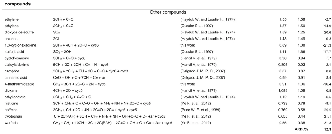
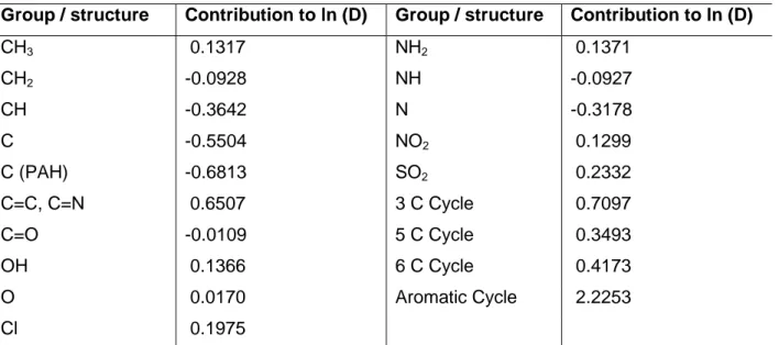
the same organic groups as pesticides, were studied (see Table 2a). They were considered to build the model. All the literature references used to build the GCM are presented in Table 2a. Some supplementary measurements were done in the present work to estimate the contribution of organic functions not present in the literature data. They are also presented in Table 2a. 129 experimental diffusion coefficients of 93 organic molecules in water at 25°C were finally considered. This selection will be referred as 'the reference set' in the text. From these data, the contribution of the different organic fragments to the diffusion coefficient was estimated. For that purpose, the molecules were first divided in organic functions (as presented in Table 2a) and the contributions of each group were estimated by an iterative process and minimisation (least squares regression) of the difference between the experimental and calculated diffusion coefficients. The contribution of each group is presented in Table 2b. To check the applicability of the method and evaluate its precision, these contributions were then used to estimate the diffusion coefficients of a selection of pesticides referred as the test set. This set of pesticides is composed of the six pesticides studied in the present work and the pesticides studied in literature (Raveton 1999; Scott 1973) the only available data found for pesticides in literature. The results of this estimation are proposed in Table 2c and discussed in the results part of the paper.
Multimedia environmental models
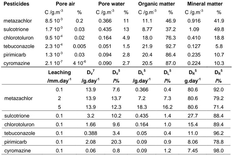
A three compartments (soil, water, air) multimedia fate model based on the fugacity approach (surface soil model) was implemented to estimate the fate of different pesticides present in soil. The model used was developed by Mackay (Mackay 2001) and details of the calculations can be found in the work of Jury et al. (Jury 1983). The soil considered is composed of organic and mineral matter, water and air. Its exact composition and characteristic sizes are given in Table 3. This soil is in contact with air and a known quantity (1 kg/ha) of a pesticide was introduced in it. Different leaching were considered varying from 0.1 mm.day-1 to 5 mm.day-1. The pollutant is removed from the soil through three processes: volatilization, leaching and chemical/biochemical transformation. The total rate of pesticide removal corresponds to the sum of these three contributions. The model was used to describe the partition of the pesticide considered to be at equilibrium in the different parts of the soil and estimate the importance of each of these processes.
The properties necessary to predict the chemical loss from soils are: (i) the partition coefficients (octanol-water partition, Henry's law constant, organic carbon-water, organic matter- water, mineral matter-water), (ii) the degradation coefficients (degradation half time in soil, DT50) and (iii) the diffusion coefficients (molecular diffusivity in air and in water). These physico-chemical properties are given in Table 1 for the six pesticides. DR, Dv and DL are the fluxes corresponding to the removal of the pesticide by reaction,
volatilization and leaching respectively. The volatilization flux, Dv, is calculated from the
diffusion flux in the air pores, DA, and in water pores, DW, of the soil and of the interfacial
air-water diffusion, DE, according to:
Eq 8 (8)
DA is calculated from ZA, the fugacity capacity of the pesticide in the air (Z value in air),
DEA, the effective diffusivity of the pesticide in air, Y, the diffusion path length
corresponding to the distance from the position of the pesticide to the soil surface and A, the interface area, according to :
Eq 9 (9)
DEA is estimated from the diffusivity in air, DAir, taken as a constant value (4.98.10-6 m2.s -1
) and considering the tortuosity using the Millington Equation (Jury 1983):
Eq 10 (10)
with vA the volume of the air pores and vw the volume of the water phase in the soil.
Dw is calculated with the same procedure according to :
Eq 11 (11)
Eq 12 (12)
with DEW, the effective diffusivity in water, ZW the fugacity capacity on the pesticide in
water and Dwater the diffusivity in water (coefficient measured and estimated in the
present work)
The interfacial air-water diffusion, DE, is obtained from air-water mass transfer coefficient,
kv, according to:
Eq 13 (13)
with kv estimated from the air diffusivity, DAir and the air boundary layer thickness, ABL
according to :
Eq 14 (14)
The influence of measured or estimated diffusion coefficient on the fate of the studied pesticides are presented in the next section.
RESULTS AND DISCUSSION
It was explored in this work different ways to obtain diffusion coefficients of a pesticide infinitely diluted in water. First, these coefficients were experimentally measured and then estimated with empirical equations and GCM model.
Experimental determination of diffusion coefficients
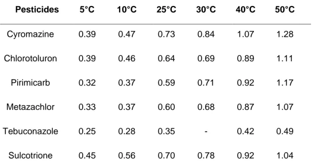
In Table 4 are listed the experimental values of molecular diffusion coefficients for the studied pesticides as a function of temperature (T= 5, 10, 25, 30, 40 and 50°C). At room temperature (25°C), the lower diffusivity, 0.35 × 10⁻⁹ m2.s-1, is obtained for tebuconazole. No literature data was found for comparison. However, the diffusion coefficient measured for tebuconazole is comparable to those obtained for the diffusion of heavy polycyclic aromatic hydrocarbons at 25°C in water like anthracene (three aromatic cycles, 0.418 × 10⁻⁹ m2.s-1) and benzanthracene (four aromatic cycles, 0.335 × 10⁻⁹ m2.s-1) (Gustafson and Dickhut 1994). It is one order of magnitude higher than the diffusion coefficient of atrazine in water of 0.26 × 10⁻¹⁰ m2.s-1 measured by Raveton et al. (Raveton et al 1999). For the other studied pesticides, diffusivities are higher, varying at 25°C from 0.59 × 10⁻⁹ m2.s-1 for pirimicarb to 0.73 × 10⁻⁹ m2.s-1 for cyromazine. These values are comparable to the diffusion coefficients measured by Scott and Phillips (Scott 1973) for another selection of pesticides (diffusion coefficients ranging from 0.58 to 0.68 × 10⁻⁹ m2.s-1). The coefficients measured for these pesticides are also comparable to the diffusivity of naphthalene, composed of two aromatic cycles (0.749 × 10⁻⁹ m2.s-1) (Gustafson and Dickhut 1994). Ibuprofen (0.713 × 10⁻⁹ m2.s-1) (Ye et al 2012), paracetamol (0.664 × 10⁻⁹ m2.s-1) (Ribeiro et al 2012), both containing one aromatic cycle and leucine (0.735 × 10⁻⁹ m2.s-1) (Umecky 2006) also present similar diffusion coefficients in water.
The diffusivity is function of the environmental conditions in particular the temperature. As observed in Table 4, an increase of temperature from 5 to 50°C increases the diffusion coefficient by a factor 2 (case of tebuconazole) to 3.5 (case of pirimicarb). The diffusion is also dependant on the size of the diffusing specie. In the present study, for example, cyromazine has the lower molar mass (166 g.mol-1) and, as expected, also the highest diffusion coefficient. However, it is not possible to establish a direct relationship between the molar mass of the pesticide and its diffusion coefficient in water because other parameters like the interactions between the solute and the solvent influence the mobility of the solute in the medium.
The validity of the Stokes-Einstein equation was tested for the considered systems. For that purpose, for each pesticide, the experimental diffusion coefficients were fitted as a function of T/. We assume a constant hydrodynamic radius as a function of temperature. The results obtained are given in Table 5. The standard error of the estimate (SEE) is the standard deviation between the experimental and calculated diffusion coefficients and gives an indication of the validity of the equation to fit our experimental data. Except for tebuconazole and sulcotrione, the two pesticides with the highest molar masses, for which SEE represent more than 20% of the diffusion coefficient, acceptable results are obtained for all the pesticides (SEE is 12% of the diffusion coefficient in the case of pirimicarb, the worse case). Deviations from Stoke-Einstein's equation can be explained by a non-applicability of the assumptions of this equation (for example the sphericity of the diffusing specie).
Estimation of diffusion coefficients
The three empirical models presented above were used to calculate molecular diffusion coefficients of the six pesticides in water at different temperatures and compared to experimental data. All the results are presented in Table 6.
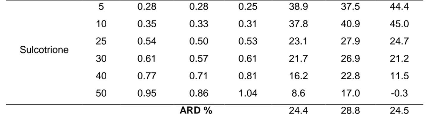
For the four smaller molecules (cyromazine, chlorotoluron, pirimicarb and metazachlor), the three equations leads to acceptable estimation of the diffusion coefficients. The Wilke-Chang equation gives the best results for these pesticides with average relative deviation varying from 1.3% for cyromazine to 9.8% for metazachlor. With equations 6 and 7, average relative deviations vary from 7.1 % (cyromazine, equations 6 and 7) to 13.5% (pirimicarb, equation 6). At lower temperatures, using eq 7, the diffusion coefficient is underestimated while it is overestimated (or at least less underestimated) at higher temperatures. The estimated molecular diffusion coefficients are unsatisfactory for tebuconazole and sulcotrione, the two heaviest pesticides considered (average relative deviations between 25 and 36%). This may be explained by a molar volume not correctly estimated for example because no temperature dependency is considered and because of the absence of some functional groups present in pesticides (in particular aromatic cycles) in the Le Bas additivity constants.
Group Contribution Methods (GCM) is another way of estimating the diffusivity of pesticides when experimental data are not available for the studied pesticide. The contribution of the organic groups that constitute pesticides were calculated in the
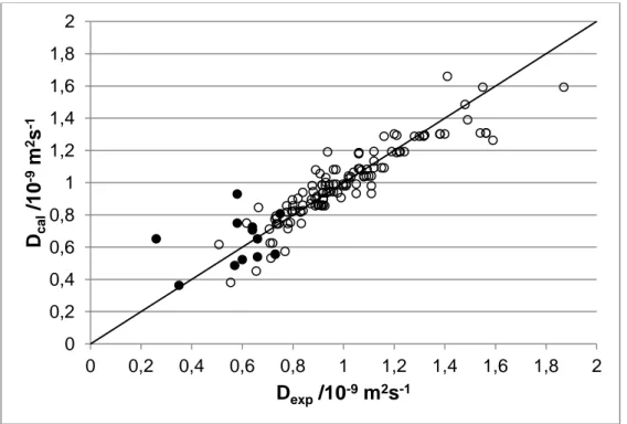
present work as previously described (see Table 2b). The applicability of the GCM was then tested on a selection of pesticides for which experimental diffusion coefficients are available. This selection, referred as the 'test set', is composed of the pesticides studied in the present work and those studied by Scott et al. (Scott 1973) and Raveton et al. (Raveton 1999). The experimental and calculated diffusion coefficients are presented in Table 2c. The relative deviations between the experimental and calculated coefficients are acceptable for most of the pesticides. For atrazine, an important deviation between the literature data is observed. For this component, the estimated diffusion coefficient is three times higher than the value measured by Raveton (Raveton 1999) while it corresponds (1% of relative deviation) to the value measured by Scott (Scott 1973). The deviations with the values of Scott et al. (Scott 1973) are comparable to the precision given by the authors in their study so it is difficult to conclude on the precision of the GCM with this comparison. Finally, the average RD between the present experimental data and the predictions with the GCM is less than 15%. This will be considered as the precision of the estimation method. In Figure 1, it can be observed graphically the deviation between experimental and calculated data. It can also be seen that most of the data of the reference set (used to establish the contribution of each fragment) correspond to diffusion coefficients higher than 0.8 × 10⁻⁹ m2.s-1 probably because the solute considered are small molecules. Far less data are available in the range of the diffusion coefficients of pesticides. The model could thus be highly improved with the introduction of new sets of experimental data in the range 0.2 - 0.8 × 10⁻⁹ m2.s-1.
Finally, we have considered that the GCM developed here can be used for pesticides leading to a precision of the diffusion coefficients of 15%. Alternatively, correlation equations (equations 5, 6 and 7) lead to precisions of typically less than 10% but are not equally efficient for all the pesticides considered.
Multimedia environmental Model Set-up: Impact of diffusion coefficient on fate The second objective of this study is to see how the diffusivity of a pesticide in water affects the estimation of its environmental fate. For that purpose, a multimedia environmental model, based on the fugacity approach was used with a focus on its sensitivity to the values of the diffusion coefficients. A surface soil model was selected for this work. Indeed, pesticides are frequently present in surface soils as a consequence of the application of agrochemicals. The model estimates the time needed for the complete elimination of this chemical. Our aim is to evaluate the impact of the precision of the
diffusion coefficient on the previsions of the environmental fate. For that purpose, while all the physico-chemical parameters and characteristics of the soil are strictly the same, differents values for the diffusion coefficient were used: (i) the experimental diffusion coefficient measured in the present work, (ii) the previous values increased or decreased by 15% this deviation corresponding to the error when estimating the coefficient using empirical/GCM models, (iii) the use of a constant value for the diffusion coefficient of all the pesticides as proposed by Jury et al (Jury 1983).
In the present case, we propose to include in these prediction schemes the experimental diffusion coefficients previously determined to estimate the environmental fate of the six pesticides studied. The only process affected by the diffusivity in water is the volatilization rate that is evaluated from the diffusion in water and air (present in the soil) and from the diffusion at the interface water-air.
All the results obtained are presented in Table 7 (distribution of the pesticide in the different parts of the soil and values of the fluxes). For all the tested pesticides, the major process responsible for the removal of the chemical is reactivity. DR, the flux
corresponding to the removal of the pesticide by reaction, is systematically at least one order of magnitude higher than Dv or DL (fluxes corresponding to the removal from
volatilization and leaching respectively) meaning about 90% of the pesticide disappears because it reacts with the environment. The removal by leaching, DL, is comparable to
volatilization, DV, this contribution being higher when the leaching is very low (typically
0.1 mm2.day-1).
In the case of highly water soluble pesticides (for example cyromazine), DA
(3.3×10⁻⁴
g.day-1) is negligible compared to DW (8.2×10⁻² g.day-1) and DE 1.9×10⁻¹
g.day-1 is in thesame order of magnitude compared to DW. It means, DE and Dw are the
limiting parameters for the determination of DV.
A 15% variation of the diffusion coefficient of the pesticide in water has no dramatic effect on the results of the predicted environmental fate, the volatilization flux being affected from 1% to 10% depending on the conditions and the pesticide. It means that the use of the GCM method developed or the use of correlation equations is sufficient for the use of a multimedia environmental model.
Jury et al. (Jury 1983) have used the same fugacity model for 2 pesticides (lindane and (2,4-dichlorophenoxy)acetic acid) with a constant value for the water diffusivity. From a compilation of experimental data on organic compounds, an average value of 4.98 × 10⁻¹⁰ m2.s-1 was chosen as representative of all the pesticides. This value is the
same order of magnitude as the experimental data measured in the present work. Even though, the use of a constant value can, in certain cases, greatly affect the results. For example, in the case of cyromazine, the volatilization flux is affected by 25% (4.3×10⁻²
g.day-1 instead of 5.7×10⁻² g.day-1) when using a value of 4.98 ×10⁻¹⁰ m2.s-1 for the water diffusivity as proposed by Jury et al. instead of 0.73 ×10⁻⁹ m2.s-1 (value measured in the present work).
CONCLUSION
Diffusion in water is an important parameter for the estimation of environmental fate of pesticides when advection is not dominant. Experimental data for the diffusion of pesticides are scarce in literature and often a constant value for the diffusivity in water is considered in models. In the present work, we present original experimental diffusion data of six pesticides infinitely diluted in water, measured using the Taylor dispersion technique, with a precision of 3% as a function of temperature from 5 to 50°C. We also discuss the possibility to estimate these coefficients. Diffusion coefficients are function of the diffusing specie and also of the solvent in which it is diffusing (and of their interactions). It is a difficult task to precisely predict these parameters. Correlation equations (developed for organic components) are efficient to predict the diffusion of pesticides with a precision of typically 10%. For some pesticides, the predicted values are less precise probably an inaccurate knowledge of molar volume. Alternatively, a group contribution method was built in the present work, using a large set of literature data, leading to 15% precision results. With the collection of new experimental data sets, it could even be possible to highly improve the precision of this GCM method.
The second objective of the work was to introduce the diffusion coefficients in a soil model and evaluate the impact of their precision on the results of the model. The precision obtained with the GCM values was proved to be sufficient for use in environmental models. The introduction of an experimental or calculated value for the diffusion coefficient thus different for each pesticide is an improvement compared to the use of a constant value as often proposed in literature. The use of a constant value for the diffusion coefficient, as sometimes proposed in literature, can induce large errors (up to 25%) on the environmental fate.
The authors thank the Regional Auvergne Council, CNRS, the French Ministry of Higher Education and Research and the European Regional Developement Fund for financial support to buy the diffusion coefficient equipment. The authors acknowledge Philippe Bouchard for giving tebuconazole samples.
References:
Ali I, Jain CK (1998) Groundwater contamination and health hazards by some of the most commonly used pesticides. Current Science 75:1011-1014.
Ali I, Singh P, Rawat MSM, Badoni A (2008) Analysis of organochlorine pesticides in the Hindon river water, India. Journal of Environmental Protection Science 2:47-53.
Alizabeth A, Nieto de Castro CA, Wakeham WA (1980) The theory of the Taylor dispersion technique for liquid diffusivity measurements. International Journal of thermophysics 1:243-283.
Batiha MA, Kadhum AAH, Mohamad AB, Takriff MS, Fisal Z, Wan Daud WR, Batiha MM (2009) Modeling the fate and transport of non-volatile organic chemicals in the agro-ecosystem: A case study of Cameron Highlands, Malaysia. Process Savety and Environmental Protection 87:121-134.
Baum EJ (1998) Chemical property estimation: Theory and application. Lewis Publishers, Boca Raton, USA.
Bonoli L, Witherspoon PA (1968) Diffusion of aromatic and cycloparaffin hydrocarbons in water from 2 to 60°. J. Phys. Chem. 72:2532-2534.
Camenzuli L, Scheringer M, Gaus C, Ng CA, Hungerbuhler K (2012) Describing the environmental fate of diuron in a tropical river catchment. Science of the total Environment 440:178-185.
Cussler EL (1997) Diffusion Mass Transfer in Fluids systems. Cambridge University Press, Cambridge UK.
Delgado JMPQ (2007) Molecular diffusion coefficients of organic compounds in water at different temperatures. Journal of Phase Equilibria and Diffusion 28:427-432.
Easteal AJ, Woolf LA (1985) Pressure and temperature dependance of tracer diffusion coefficients of methanol, ethanol, acetonitrile and formamide in water. J. Phys. Chem. 89:1066-169.
Funazukuri T, Nishio M (1999) Infinite dilution binary diffusion coefficients of C5-monoalcohols in water in the temperature range from 273.2 K to 353.2 K at 0.1 MPa. J. Chem. Eng. Data 44:73-76.
Gary-Bobo CM, Weber HW (1969). Diffusion of alcohols and amides in water. The Journal of Physical Chemistry 73:1155-1156.
Gosting LJ, Akeley DF (1952) A study of the diffusion of urea in water at 25° with the Gouy interference method. J. Am. Chem. Soc. 74:2058-206.
Gustafson KE, Dickhut RM (1994). Molecular diffusivity of polycyclic aromatic hydrocarbons. J. Chem. Eng. Data 39:281-285.
Hancil V, Rod V, Rosenbaun M (1979) Diffusivity determination from the response to injection into laminar liquid flow in a capillary. Chem. Eng. Commun. 3:155-163.
Hao L, Leaist DG (1996) Binary mutual diffusion coefficients of aqueous alcohols. Methanol to 1-heptanol. J. Eng. Chem. Data 41:210-213.
Harris KR (1991) On the use of the Edgeworth-Cramer series to obtain diffusion coefficients from Taylor dispersion peaks. J. Sol. Chem. 20:595-606.
Harris KR, Goscinska T, Lam HN (1993) Mutual diffusion coefficients for the systems water-ethanol and water-propan-1-ol at 25°C. J. Chem. Soc. Faraday Trans. 89:1969-1974.
Harris KR, Lam HN (1995) Mutual diffusion coefficients and viscosites for the water-2-methylpropan-2-ol system at 15 and 25°C. J. Chem. Soc. Faraday Trans. 91:4071-4077. Hayduk W, Laudie H (1974) Prediction of diffusion coefficients for nonelectrolytes in dilute aqueous solutions. AIChE J. 20:611-615.
Jury WA, Spencer WF, Farmer WJ (1983) Behavior assessment model for trace organics in soil: I. Model description. J. Environ. Qual. 12:558-564.
Katagi T, Ose K (2015) Toxicity, bioaccumulation and metabolism of pesticides in the earthworm. Journal of Pesticides Science 40:69-81.
Kaushik P, Kaushik G (2007) An assessment of sructure and toxicity correlation in organochlorine pesticides. Journal of hazardous Materials 143:102-111.
Lampreia IMS, Santos AFS, Barbas MJA, Santos FJS, Matos Lopes MLS (2007) Changes in aggregation patterns detected by diffusion, viscosity, and surface tension in water + 2-(diethylamino)ethanol mixtures at different temperatures. J. Chem. Eng. Data 52:2388-2394.
Luo Y, Zhang M (2009) Multimedia transport and risk assessment of organophosphate pesticides and a case study in the northern San Joaquin Valley of California. Chemosphere 75:969-978.
Ma YG, Lei Y, Xiao H, Wania F, Wang WH (2010) Critical review and recommended values for Physical-Chemical property data of 15 polycyclic aromatic hydrocarbons at 25°C. J. Chem. Eng. Data 55:819-825.
Mackay D (2001) Multimedia Environment Models, the fugacity Approach, 2nd Edition. CRC Taylor and Francis, Boca Raton.
Malanichev A, Mantseva E, Shatalov V, Strukhov A, Vulikh N (2004) Numerical evaluation of the polychlorinated biphenyls transport over the nothern hemisphere. Environ. Poll. 128:279-289.
Mrema EJ, Rubino FM, Brambilla G, Moretto A, Tsatsakis AM, Colosio C (2013) Persistent organochlorinated pesticides and mechanisms of their toxicity. Toxixology 307:74-88.
Muir DCG, Teixeira C, Wania F (2004) Empirical and modeling evidence of regional atmospheric transport of current-use pesticides. Environ. Toxicol. Chem. 23:2421-2432. Niesner R, Heintz A (2000) Diffusion coefficients of aromatics in aqueous solution. J. Chem. Eng. Data 45:1121-1124.
Otto S, Pappalardo SE, Cardinali A, Masin R, Zanin G, Borin M (2016) Vegetated Ditches for the Mitigation of Pesticides Runoff in the Po Valley. PLoS ONE 11.
Othmer DF, Thakar MS (1953) Correlating diffusion coefficients in liquids. Ind. Eng. Chem. 45:589-593.
Price WE, Trickett KA, Harris KR (1989) Association of caffeine in aqueous solution. J. Chem. Soc. Faraday Trans. 85:3281-3288.
Raveton M, Schneider A, Deprez-Durand C, Ravanel P, Tissut M (1999) Comparative diffusion of atrazine inside aqueous or organic matices and inside plant seedings. Pestic. Biochem. Physiol. 65:36-43.
Ribeiro ACF, Barros MCF, Verissimo LMP, Santos CIAV, Cabral AMTDPV, Gaspar GD, Esteso MA (2012) Diffusion coefficients of paracetamol in aqueous solutions. J. Chem. Thermodyn. 54:97-99.
Sarraute S, Costa Gomes MF, Padua AAH (2009) Diffusion coefficients of 1-alkyl-3-methylimidazolium ionic liquids in water, methanol and acetonitrile at infinte dilution. J. Chem. Eng. Data 54:2389-2394.
Shen L, Wania F (2005) Compilation, evaluation and selection of physical-chemical property data for organochlorine pesticides. J. Chem. Eng. Data 50:742-768.
Scheringer M, Wania F (2003) Multimedia models of global transport and fate of persistent organic pollutants. In: Fiedler H (ed) Hand-book of Environmental Chemistry. Springer, Berlin 237-269.
Scott HD, Phillips RE (1973) Self-diffusion coefficients of selected herbicides in water and estimates of their transmission factors in soil. Soil Sci. Soc. Amer. Proc. 37:965-967. Semeena VS, Feichter J, Lammel G (2005) Impact of the regional climate and substance properties on the fate and atmospheric long-range transport of persistent organic pollutants - Example of DDT and -HCH. Atmos. Chem. Phys. 5:12569-12615.
Shiu WY, Mackay D (1986) A critical review of aqueous solubility, vapor pressure, Henry's law constants, and octanol-water partition coefficients of polychlorinated biphenyls. J. Phys. Chem. Ref. Data 15:911-929.
Snidjer ED, Riele MJM (1993) Diffusion coefficients of several aqueous alkanolamine solutions. J. Chem. Eng. Data 38:475-480.
Stokes RH (1950a) The diffusion coefficients of eigth uni-univalent electrolytes in aqueous solution at 25°C. J. Am. Chem. Soc. 72:2243-2247.
Stokes RH (1950b) The improved diaphragm-cell for diffusion studies, and some tests of the method. J. Am. Chem. Soc. 72:763-767.
Suntio LR, Shiu WY, Mackay D, Seiber JN, Glotfelty D (1998) Critical review of Henry's law constants for pesticides. Reviews of Environmental Contamination and Toxicology 103:1-59.
Tominaga T, Matsumoto S, Ishii T (1986) Limiting interdiffusion of some aromatic hydrocarbons in water from 265 to 433 K. J. Phys Chem. 90:139-143.
Tominaga T, Matsumoto S, Takanaka JI (1984) Limiting interdiffusion coefficients of benzene, toluene, ethylbenzene and hexafluorobenzene in water from 298 to 368 K. J. Chem. Soc. Faraday Trans. 80:941-947.
Tyn MT, Calus WF (1975) Temeperature and concentration dependance of mutual diffusion coefficients of some binary liquid systems. J. Chem. Eng. Data 20:310-316. Umecky T, Kuga T, Funazukuri T (2006) Infinite dilution binary diffusion coefficients of several -amino acids in water over a temperature range from (293.2 to 333.2)K with the Taylor dispersion technique. J. Chem. Eng. Data 51:1705-1710.
Umecky T, Omori S, Kuga T, Funazukuri T (2008) Effects of hydroxyl groups on binary diffusion coefficients of -amino acids in dilute aqueous solutions. Fluid Phase Equilibria 264:18-22.
Wilke CR, Chang P (1955) Correlation of diffusion coefficients in dilute solutions. AIChE J. 1:264-270.
Witherspoon PA, Saraf DN (1965) Diffusion of methane, ethane, propane and n-butane from 25 to 43°. The Journal of Physical Chemistry 69:3752-3755.
Witherspoon PA, Saraf DN (1969) Correlation of diffusion coefficients for paraffin, aromatic, cycloparaffin hydrocarbons in water. I & EC Fundamentals 8:589-591.
Xia X, Hopke PK, Holsen TM, Crimmins BS (2011) Modeling toxaphene behavior in the great lakes. Science of Total Environment 409:792-799.
Ye F, Jensen H, Larsen SW, Yaghmur A, Larsen C, Ostergaard J (2012) Measurement of drug diffusivities in pharmaceutical solvents using Taylor dispersion analysis. Journal of Pharmaceutical and biomedical analysis 61:176-183.
Zhang QQ, Ying GG, Chen ZF, Liu YS, Liu WR, Zhao JL (2015) Multimedia fate modeling and risk assessment of a commonly used azole fungicide climbazole at the river basin scale in China. Science of Total Environment 520:39-48.
Name CAS Number
Formula
Molecular structure Purity /% Mw /g.mol-1 Sw /mg.L-1 VP1 /mPa Log KOW1 DT501 /days Koc1 *Kfoc Kmw1 /L.kg-1 Cyromazine 66215-27-8 C6H10N6 99.8 166.2 13000 4.48 10-4 0.069 93 409* 1 Chlorotoluron 15545-48-9 C10H13ClN2O 99.7 212.3 74 5.00 10-3 2.5 45 196 1 Pirimicarb 23103-98-2 C11H18N4O2 99.0 238.4 3100 0.43 1.18 86 388* 1 Metazachlor 67129-08-2 C14H16ClN3O 99.9 277.8 450 0.093 2.49 8.6 54 1 Tebuconazole 107534-96-3 C16H22ClN3O 99.6 307.8 36 1.30 10-3 3.7 63 769*
Chemical properties are found in PPDB (http://sitem.herts.ac.uk/aeru/ppdb/en/index.htm) database and are used as parameters
Sulcotrione 99105-77-8 C14H13ClO5S
98.8 328.8 165.0 5.00 10-3 -1.7 25 36*
D /10-9 m2.s-1 Organic
compounds
Group /structure reference Dexp Dcalc RD3 (%)
Alkanes
ethane 2CH3 (Hayduk W. and Laudie H., 1974) 1.38 1.30 5.7
ethane 2CH3 (Cussler E.L., 1997) 1.20 1.30 -8.5
propane 2CH3 + CH2 (Witherspoon P. A. and Saraf D. N., 1965) 1.21 1.19 2.0
chloromethane CH3 + Cl (Hayduk W. and Laudie H., 1974) 1.49 1.39 6.7
n-butane 2CH3 + 2CH2 (Witherspoon P. A. and Saraf D. N., 1965) 0.96 1.08 -12.6
n-butane 2CH3 + 2CH2 (Hayduk W. and Laudie H., 1974) 0.97 1.08 -11.4
ARD /% 7.8
Alcohols
methanol CH3 + OH (Easteal A. J. and Woolf L. A., 1985) 1.56 1.31 16.3
methanol CH3 + OH (Harris K. R. et al., 1993) 1.56 1.31 16.3
methanol CH3 + OH (Hao L. and Leaist D. G., 1996) 1.54 1.31 15.1
ethanol CH3 + CH2 + OH (Hayduk W. and Laudie H., 1974) 1.24 1.19 3.9
ethanol CH3 + CH2 + OH (Easteal A. J. and Woolf L. A., 1985) 1.22 1.19 2.6
ethanol CH3 + CH2 + OH (Harris K. R. et al., 1993) 1.22 1.19 2.6
ethanol CH3 + CH2 + OH (Hao L. and Leaist D. G., 1996) 1.22 1.19 2.3
1-propanol CH3 + 2CH2 + OH (Harris K. R. et al., 1993) 1.064 1.09 -2.1
1-propanol CH3 + 2CH2 + OH (Hao L. and Leaist D. G., 1996) 1.059 1.09 -2.6 isopropanol 2CH3 + CH + OH (Hayduk W. and Laudie H., 1974) 1.080 1.04 4.0 isopropanol 2CH3 + CH + OH (Hao L. and Leaist D. G., 1996) 1.029 1.04 -0.7 ethylene glycol 2CH2 + 2OH (Hayduk W. and Laudie H., 1974) 1.160 1.10 5.9 butan-2-ol 2CH3 + CH2 + CH + OH (Hao L. and Leaist D. G., 1996) 0.94 0.94 -0.4 isobutanol 2CH3 + CH2 + CH + OH (Hao L. and Leaist D. G., 1996) 0.95 0.94 0.6 t-butanol 3CH3 + C + OH (Harris K. R. and Lam H. N., 1995) 0.93 0.98 -5.7
t-butanol 3CH3 + C + OH (Hao L. and Leaist D. G., 1996) 0.88 0.98 -12.1
butan-1-ol CH3 + 3CH2 + OH (Hancil V. et al., 1979) 0.971 0.99 -1.9
butan-1-ol CH3 + 3CH2 + OH (Hao L. and Leaist D. G., 1996) 0.96 0.99 -3.1 pentan-1-ol CH3 + 4CH2 + OH (Hao L. and Leaist D. G., 1996) 0.888 0.90 -1.6 pentan-1-ol CH3 + 4CH2 + OH (Funazukuri T. and Nishio M., 1999) 0.920 0.90 2.0 pentan-2-ol 2CH3 + 2CH2 + CH + OH (Funazukuri T. and Nishio M., 1999) 0.911 0.86 5.5
D /10-9 m2.s-1 Organic
compounds
Group /structure reference Dexp Dcalc RD (%)
pentan-3-ol 2CH3 + 2CH2 + CH + OH (Funazukuri T. and Nishio M., 1999) 0.899 0.86 4.2 3-methyl-1-butanol 2CH3 + 2CH2 + CH + OH (Funazukuri T. and Nishio M., 1999) 0.903 0.86 4.7 2-methyl-1-butanol 2CH3 + 2CH2 + CH + OH (Funazukuri T. and Nishio M., 1999) 0.920 0.86 6.4 3-methyl-2-butanol 2CH3 + 2CH2 + CH + OH (Funazukuri T. and Nishio M., 1999) 0.899 0.86 4.2 2-methyl-2-butanol 2CH3 + CH2 + C+ OH (Funazukuri T. and Nishio M., 1999) 0.873 0.89 -2.5 2,2-dimethyl-1-propanol 2CH3 + CH2 + C+ OH (Funazukuri T. and Nishio M., 1999) 0.920 0.89 2.8 hexan-1-ol CH3 + 5CH2 + OH (Hao L. and Leaist D. G., 1996) 0.830 0.82 1.0 heptan-1-ol CH3 + 6CH2 + OH (Hao L. and Leaist D. G., 1996) 0.800 0.85 -7.0
ARD4 /% 4.8
Amines-amides-ketones-carboxilic acids
ethylamine CH3 + CH2 + NH2 this work 1.19 1.19 -0.2
acetone 2CH3 + C=O (Hayduk W. and Laudie H., 1974) 1.28 1.29 -0.6
acetone 2CH3 + C=O (Tyn M. T. and Calus W. F., 1975) 1.30 1.29 1.0
acetone 2CH3 + C=O (Hancil V. et al., 1979) 1.316 1.29 2.2
acetone 2CH3 + C=O (Cussler E.L., 1997) 1.16 1.29 -11.0
acetamide CH3 + C=O + NH2 (Gary-Bobo C. M. and Weber H. W., 1969) 1.32 1.29 1.9
acetamide CH3 + C=O + NH2 (Hayduk W. and Laudie H., 1974) 1.32 1.29 1.9
acetic acid CH3 + C=O + OH (Cussler E.L., 1997) 1.21 1.29 -6.9
ethanolamine 2CH2 + NH2 + OH (Snijder E. D. and Riele M. J. M., 1993) 1.12 1.09 2.5 ethanolamine 2CH2 + NH2 + OH (Snijder E. D. and Riele M. J. M., 1993) 1.15 1.09 5.0 propanoic acid CH3 + CH2 + C=O + OH (Cussler E.L., 1997) 1.06 1.18 -11.2 butyramide CH3 + 2CH2 + C=O + NH2 (Gary-Bobo C. M. and Weber H. W., 1969) 1.07 1.08 -0.5 isobutyramide 2CH3 + CH + C=O + NH2 (Gary-Bobo C. M. and Weber H. W., 1969) 1.02 1.03 -0.6 diethanolamine 4CH2 + NH + 2OH (Snijder E. D. and Riele M. J. M., 1993) 0.84 0.83 1.6 diethanolamine 4CH2 + NH + 2OH (Snijder E. D. and Riele M. J. M., 1993) 0.808 0.83 -2.3 2-(diethylamino)ethanol 2CH3 + 4CH2 + N + OH (Lampreia I. M. S. et al., 2007) 0.617 0.75 -21.4 methyldithanolamine CH3 + 4CH2 + N + 2OH (Snijder E. D. and Riele M. J. M., 1993) 0.79 0.76 4.7 diisopropanolamine 2CH3 +2CH2 + 2CH + NH + 2OH (Snijder E. D. and Riele M. J. M., 1993) 0.71 0.63 12.0 diisopropanolamine 2CH3 +2CH2 + 2CH + NH + 2OH (Snijder E. D. and Riele M. J. M., 1993) 0.72 0.63 13.2
ARD /% 5.3
Organic compounds
Group /structure reference Dexp Dcalc RD (%)
Amino acids
urea 2NH2 + C=O (Gosting L. J. and Akeley D. F., 1952) 1.382 1.30 5.8
urea 2NH2 + C=O (Umecky T. et al., 2006) 1.40 1.30 7.1
glycine CH3 + C=O + OH + NH2 (Cussler E.L., 1997) 1.060 1.19 -11.8
glycine CH3 + C=O + OH + NH2 (Umecky T. et al., 2006) 1.061 1.19 -11.7
alanine CH3 + CH + C=O + OH + NH2 (Umecky T. et al., 2006) 0.930 1.03 -10.8 alpha-threonine CH3 + 2CH + C=O + 2OH + NH2 (Umecky T. et al., 2008) 0.796 0.82 -3.1
-amino butyric acid CH3 + CH2 + CH + C=O + OH + NH2 (Umecky T. et al., 2006) 0.839 0.94 -12.0 serine CH3 + CH + C=O + 2OH + NH2 (Umecky T. et al., 2008) 0.88 0.94 -7.3
valine 2CH3 + 2CH + C=O + OH + NH2 (Cussler E.L., 1997) 0.83 0.82 1.6
valine 2CH3 + 2CH + C=O + OH + NH2 (Umecky T. et al., 2006) 0.777 0.82 -5.1 norvaline CH3 + 2CH2 + CH + C=O + OH + NH2 (Umecky T. et al., 2006) 0.775 0.86 -10.5 homoserine 2CH2 + CH + C=O + 2OH + NH2 (Umecky T. et al., 2008) 0.839 0.86 -2.5 threonine CH3 + 2CH + C=O + 2OH + NH2 (Umecky T. et al., 2008) 0.799 0.82 -2.7 allothreonine CH3 + 2CH + C=O + 2OH + NH2 (Umecky T. et al., 2008) 0.796 0.82 -3.1 isoleucine 2CH3 + CH2 + 2CH + C=O + OH + NH2 (Umecky T. et al., 2006) 0.744 0.74 -0.1 tert-leucine 2CH3 + CH+ C + C=O + OH + NH2 (Umecky T. et al., 2006) 0.729 0.77 -6.1 alloisoleucine 2CH3 + CH2 + 2CH + C=O + OH + NH2 (Umecky T. et al., 2006) 0.738 0.74 -0.9 leucine 2CH3 + CH2 + 2CH + C=O + OH + NH2 (Umecky T. et al., 2006) 0.735 0.74 -1.3 norleucine CH3 + 3CH2 + CH + C=O + OH + NH2 (Umecky T. et al., 2006) 0.736 0.78 -6.0
ARD /% 5.8
Aromatic compounds
benzene 6CH + ar (Tominaga T. et al., 1984) 1.10 1.04 5.4
benzene 6CH + ar (Gustafson K. E. and Dickhut R. M., 1994) 1.09 1.04 4.5
benzene 6CH + ar (Cussler E.L., 1997) 1.02 1.04 -2.1
benzene 6CH + ar (Niesner R. and Heintz A., 2000) 1.08 1.04 3.6
benzene 6CH + ar (Ye F. et al., 2012) 1.11 1.04 6.2
toluene CH3 + C + 5CH + ar (Tominaga T. et al., 1984) 0.915 0.99 -7.7
toluene CH3 + C + 5CH + ar (Gustafson K. E. and Dickhut R. M., 1994) 0.915 0.99 -7.7
toluene CH3 + C + 5CH + ar (Ye F. et al., 2012) 0.943 0.99 -4.5
aniline NH2 + C + 5CH + ar (Niesner R. and Heintz A., 2000) 1.05 0.99 5.6
Organic compounds
Group /structure reference Dexp Dcalc RD (%)
phenol OH + C + 5CH + ar (Niesner R. and Heintz A., 2000) 0.998 0.99 0.7
o-cresol CH3 + OH + 2C + 5CH + ar (Niesner R. and Heintz A., 2000) 0.926 0.86 7.5 m-cresol CH3 + OH + 2C + 5CH + ar (Niesner R. and Heintz A., 2000) 0.889 0.86 3.7 p-cresol CH3 + OH + 2C + 5CH + ar (Niesner R. and Heintz A., 2000) 0.914 0.86 6.3 benzylic acohol CH2 + OH + C + 5CH + ar (Cussler E.L., 1997) 0.82 0.90 -10.1
benzoic acid C=O + OH + C + 5CH + ar (Cussler E.L., 1997) 1.00 0.98 2.0
benzoic acid C=O + OH + C + 5CH + ar (Delgado J. M. P. Q., 2007) 1.01 0.98 3.0
benzoic acid C=O + OH + C + 5CH + ar (Ye F. et al., 2012) 1.11 0.98 11.7
orcinol CH3 + 2OH + 3C + 3CH + ar (Niesner R. and Heintz A., 2000) 0.798 0.89 -11.9
naphtalene 8CH + 2C(PAH) + 2ar (Tominaga T. et al., 1986) 0.937 1.19 -27.2
2-chlorophenol OH + Cl + 2C + 4CH + ar (Niesner R. and Heintz A., 2000) 0.929 1.00 -7.9 n-butylbenzene CH3 + 3CH2 + C + 5CH + ar (Tominaga T. et al., 1986) 0.78 0.74 4.3 salicylic acid C=O + 2OH + 2C + 4CH + ar (Delgado J. M. P. Q., 2007) 1.11 0.94 16.0 salicylic acid C=O + 2OH + 2C + 4CH + ar (Ye F. et al., 2012) 1.05 0.94 11.2 2-nitrophenol OH + NO2 + 2C + 4CH + ar (Niesner R. and Heintz A., 2000) 0.977 0.94 4.3 3-nitrophenol OH + NO2 + 2C + 4CH + ar (Niesner R. and Heintz A., 2000) 0.917 0.94 -2.1 4-nitrophenol OH + NO2 + 2C + 4CH + ar (Niesner R. and Heintz A., 2000) 0.919 0.94 -1.9 4-nitrophenol OH + NO2 + 2C + 4CH + ar (Ye F. et al., 2012) 0.933 0.94 -0.4 naphtol 7CH + C + OH + 2C(PAH) + 2ar (Delgado J. M. P. Q., 2007) 1.12 1.13 -1.2
1,2-dichlorobenzene 2Cl + 2C + 4CH + ar this work 1.04 1.06 -2.4
paracetamol C=O + 2OH + 2C + 4CH + CH3 + NH + ar (Ribeiro A. C. F. et al., 2012) 0.664 0.85 -27.4
biphenyle 10CH + 2C + 2ar (Tominaga T. et al., 1986) 0.833 0.75 10.3
1-ethylnaphtalene 7CH + C + CH3 + CH2 + 2C(PAH) + 2ar (Tominaga T. et al., 1986) 0.780 0.71 8.5 phenylalanine CH2 + C + 6CH + NH2 + C=O + OH + ar (Ye F. et al., 2012) 0.707 0.71 -0.7 ibuprofen 3CH3 + CH2 + 2C + 6CH + NH2 + C=O + OH + ar (Ye F. et al., 2012) 0.713 0.53 25.5 bisphenol A OH + 4C + CH2 + 8CH + 2ar (Niesner R. and Heintz A., 2000) 0.508 0.62 -21.3
D /10-9 m2.s-1 Organic
compounds
Group /structure reference Dexp Dcalc5 RD (%)
Other compounds
ethylene 2CH2 + C=C (Hayduk W. and Laudie H., 1974) 1.55 1.59 -2.7
ethylene 2CH2 + C=C (Cussler E.L., 1997) 1.87 1.59 14.9
dioxyde de soufre SO2 (Hayduk W. and Laudie H., 1974) 1.59 1.25 20.6
chlorine 2Cl (Hayduk W. and Laudie H., 1974) 1.48 1.49 -0.3
1,3-cyclohexadiène 2CH2 + 4CH + 2C=C + cyc6 this work 0.89 1.08 -21.3
sulfuric acid SO2 + 2OH (Cussler E.L., 1997) 1.41 1.66 -17.7
cyclohexanone 5CH2 + C=O + cyc6 (Hancil V. et al., 1979) 0.96 0.94 1.7
salicylaldoxime 5CH + 2C + 2OH + C= + N + cyc6 (Hancil V. et al., 1979) 0.895 0.92 -2.1 camphor 3CH3 + 2CH2 + CH + 2C + C=O + cyc6 + cyc3 (Delgado J. M. P. Q., 2007) 0.87 0.87 0.0 cinnamic acid C=O + OH + C + 7CH + C= + ar (Delgado J. M. P. Q., 2007) 0.99 0.91 8.4
4-methylimidazole CH3 + 3CH + 2C=C + 2N + cyc5 this work 0.91 1.06 -16.4
dioxane 4CH2 + 2O + cyc6 (Hancil V. et al., 1979) 1.093 1.09 0.9
ethyl acetate 2CH3 + CH2 + C=O + O (Hayduk W. and Laudie H., 1974) 1.12 1.19 -6.5 histidine 3CH + CH2 + C + C=O + OH + NH2 + NH + N+ 2C=C + cyc5 (Ye F. et al., 2012) 0.733 0.79 -8.1 caffeine 3CH3 + CH + 2C + 4N + 2C=O + 2C= + cyc6 + cyc5 (Price W. E. et al., 1989) 0.769 0.58 25.5 tryptophan C + 2C(PAH) + 6CH + CH2 + NH2 + NH + OH +C=O + C= +ar + cyc5 (Ye F. et al., 2012) 0.655 0.44 31.1 warfarin CH3 + CH2 + 10CH + 3C + 2C(PAH) + 2C=O + OH + O + C= + 2ar + cyc6 (Ye F. et al., 2012) 0.55 0.38 31.3
ARD /% 12.3
Group / structure Contribution to ln (D) Group / structure Contribution to ln (D) CH3 0.1317 NH2 0.1371 CH2 -0.0928 NH -0.0927 CH -0.3642 N -0.3178 C -0.5504 NO2 0.1299 C (PAH) -0.6813 SO2 0.2332 C=C, C=N 0.6507 3 C Cycle 0.7097 C=O -0.0109 5 C Cycle 0.3493 OH 0.1366 6 C Cycle 0.4173 O 0.0170 Aromatic Cycle 2.2253 Cl 0.1975
D /10-9 m2.s-1
Organic compounds Group /structure reference Dexp Dcalc RD (%)
PESTICIDES (test set)
atrazine 3CH3 + 3N + 2NH + CH + CH2 + 3C + Cl + ar (Raveton M. et al., 1999) 0.26 0.66 -150.5 atrazine 3CH3 + 3N + 2NH + CH + CH2 + 3C + Cl + ar (Raveton M. et al., 1999) 0.666 0.66 1.3 simazine 2CH3 + 3N + 2NH + 2CH2 + 3C + Cl + ar (Raveton M. et al., 1999) 0.58* 0.75 -29.1 chlorpropham 2CH3 + C=O + NH + 5CH + 2C + Cl + O + ar (Raveton M. et al., 1999) 0.64
2
0.72 -13.2 2,4-Dichlorophenoxyacetic acid CH2 + C=O + OH + 3CH + 3C + 2Cl + O + ar (Raveton M. et al., 1999) 0.582 0.93 -60.2 prometone 5CH3 + 3N + 2NH + 2CH + 3C + O + ar (Raveton M. et al., 1999) 0.662 0.54 18.3 diphenamid 2CH3 + N + 11CH + 2C + C=O + 2ar (Raveton M. et al., 1999) 0.572 0.49 14.7 cyromazine 2NH2 + 3C + 3N + NH + 4 CH2 + 2CH + ar + cyc3 this work 0.73 0.56 23.9 chlorotoluron 3CH3 + N + C=O + NH + 3CH + 3C + Cl + ar this work 0.64 0.71 -10.4 pirimicarb 6CH3 + 4 N + 4C + C=O + O + ar this work 0.59 0.65 -9.5 metazachlor 2CH3 + 2CH2 + 6CH + 3C + 3N +2C= + C=O + Cl + ar + cyc5 this work 0.60 0.52 13.3 tebuconazole 3CH3 + 3CH2 + 6CH + 4C + 3N +2C= + OH + Cl + ar + cyc5 this work 0.35 0.36 -3.1 sulcotrione CH3 + 3CH2 + 4CH + 3C + 3C=O + Cl + SO2 + ar + cyc6 this work 0.70 0.79 -13.3
Area /m2 Depth /m Diffusion Path Length /m Volumic fraction of air Volumic fraction of water Air boundary layer thickness /m 1000 0.100 0.0500 0.2 0.3 4.75 10-3 Density /kg.m-3
air water Organic matter Mineral matter
1.19 1000 1000 2500
Mass fraction of organic carbon in dry soil Mass fraction of organic carbon in organic matter
0.02 0.56
Table 3. Characteristics lengths and composition of the soil considered for the model. Pesticides 5°C 10°C 25°C 30°C 40°C 50°C Cyromazine 0.39 0.47 0.73 0.84 1.07 1.28 Chlorotoluron 0.39 0.46 0.64 0.69 0.89 1.11 Pirimicarb 0.32 0.37 0.59 0.71 0.92 1.17 Metazachlor 0.33 0.37 0.60 0.68 0.87 1.07 Tebuconazole 0.25 0.28 0.35 - 0.42 0.49 Sulcotrione 0.45 0.56 0.70 0.78 0.92 1.04
Pesticides a /10-15 Pa.m2.K-1 s Cyromazine 2.190.01 1.3 Chlorotoluron 1.890.04 3.4 Pirimicarb 1.900.04 3.8 Metazachlor 1.800.01 1.0 Tebuconazole 0.930.08 6.0 Sulcotrione 2.00.1 9.4
Dcalc /10-9 m2.s-1 RD (%) Pesticides t /°C Eq (5) Eq (6) Eq (7) Eq (5) Eq (6) Eq (7) Cyromazine 5 0.40 0.38 0.34 -2.0 2.8 14.0 10 0.47 0.45 0.41 0.2 5.1 12.2 25 0.73 0.68 0.71 0.6 6.8 3.2 30 0.82 0.77 0.82 2.0 8.5 1.9 40 1.04 0.96 1.09 2.9 10.5 -2.0 50 1.28 1.16 1.40 -0.1 9.0 -9.3 ARD % 1.3 7.1 7.1 Chlorotoluron 5 0.35 0.33 0.29 10.7 14.9 24.5 10 0.41 0.39 0.36 10.7 15.1 21.3 25 0.64 0.60 0.62 0.8 6.9 3.1 30 0.72 0.67 0.72 -4.5 2.5 -4.9 40 0.91 0.84 0.96 -2.2 5.8 -7.6 50 1.12 1.02 1.23 -1.0 8.2 -10.6 ARD % 5.0 8.9 12.0 Pirimicarb 5 0.31 0.30 0.26 3.2 7.7 17.9 10 0.37 0.35 0.32 1.2 6.1 12.7 25 0.57 0.53 0.55 4.2 10.1 6.3 30 0.64 0.60 0.65 9.6 15.7 9.1 40 0.81 0.75 0.85 12.0 18.9 7.2 50 1.00 0.91 1.09 14.7 22.5 6.4 ARD % 7.5 13.5 9.9 Metazachlor 5 0.30 0.28 0.25 10.4 14.6 24.0 10 0.35 0.33 0.31 5.7 10.4 16.7 25 0.54 0.50 0.53 10.3 15.8 12.2 30 0.61 0.57 0.62 10.0 16.0 9.4 40 0.77 0.71 0.82 11.2 18.2 6.3 50 0.95 0.87 1.05 11.0 19.1 2.3 ARD % 9.8 15.7 11.8 Tebuconazole 5 0.27 0.26 0.23 -7.2 -2.2 8.9 10 0.32 0.30 0.28 -12.9 -7.3 0.0 25 0.49 0.46 0.48 -39.7 -31.0 -37.0 40 0.70 0.65 0.74 -66.7 -53.6 -76.3 50 0.86 0.78 0.95 -76.1 -60.1 -93.8 ARD % 33.8 25.7 36.0
Sulcotrione 5 0.28 0.28 0.25 38.9 37.5 44.4 10 0.35 0.33 0.31 37.8 40.9 45.0 25 0.54 0.50 0.53 23.1 27.9 24.7 30 0.61 0.57 0.61 21.7 26.9 21.2 40 0.77 0.71 0.81 16.2 22.8 11.5 50 0.95 0.86 1.04 8.6 17.0 -0.3 ARD % 24.4 28.8 24.5
Pesticides Pore air Pore water Organic matter Mineral matter C /g.m-3 % C /g.m-3 % C /g.m-3 % C /g.m-3 % metazachlor 8.5 10-3 0.2 0.366 11 11.1 46.9 0.916 41.9 sulcotrione 1.7 10-3 0.03 0.435 13 8.77 37.2 1.09 49.8 chlorotoluron 9.5 10-4 0.02 0.164 4.9 18.0 76.3 0.410 18.8 tebuconazole 2.3 10-4 0.005 0.051 1.5 21.9 92.7 0.127 5.8 pirimicarb 1.3 10-3 0.03 0.094 2.8 20.4 86.4 0.235 10.7 cyromazine 2.1 10-7 4 10-6 0.090 2.7 20.5 87.0 0.224 10.3 Leaching /mm.day-1 DV7 /g.day-1 DV5 /% DL5 /g.day-1 DL5 /% DR5 g.day-1 DR5 /% metazachlor 0.1 13.9 7.6 0.366 0.4 80.6 92.0 2 13.9 13.7 7.2 7.3 80.6 79.2 5 13.9 12.3 18.3 16.2 80.6 71.4 sulcotrione 0.1 3.2 10.2 0.435 1.4 27.7 88.4 chlorotoluron 0.1 1.66 9.6 0.164 1.0 15.4 89.4 tebuconazole 0.1 0.388 3.4 0.05 0.4 11.0 96.2 pirimicarb 0.1 2.08 20.3 0.09 0.9 8.06 78.8 cyromazine 0.1 0.06 0.8 0.09 1.2 7.45 98.0
Table 7. Partition of the pesticides in the different parts of the soil for a chemical
dose of 1 kg/ha a) mass concentrations with a leaching of 0.1 mm.day-1 b) removal
fluxes and different leaching.
Figure 1: Infinite dilution diffusion coefficients at 25°C. Experimental values versus those predicted with the group contribution scheme: reference set,
test set 0 0,2 0,4 0,6 0,8 1 1,2 1,4 1,6 1,8 2 0 0,2 0,4 0,6 0,8 1 1,2 1,4 1,6 1,8 2 Dcal /1 0 -9 m 2 s -1 Dexp /10-9 m2s-1