Computationally efficient modelling for long term prediction of global positioning system orbits.

T-640

COMPUTATIONALLY EFFICIENT MODELLING FOR LONG TERM PREDICTION OF GLOBAL

POSITIONING SYSTEM ORBITS by

Sean Kevin Collins

B. S. A. E., UNIVERSITY OF VIRGINIA (1974)

SUBMITTED IN PARTIAL FULFILLMENT OF THE REQUIREMENTS FOR THE DEGREE OF

MASTER OF SCIENCE IN AERONAUTICS AND ASTRONAUTICS at the

MASSACHUSETTS INSTITUTE OF TECHNOLOGY February, 1977

Signature of Author_ ___ _ _ _ Department of Aeronautics and Astronautics, Feb., 1977 Certified by Certified by Accepted by

ARCHIVES

FEB

16 1977

brsraes Thesis Supervisor Th'Evsis- Supervisok Chairman, Departmental Graduate Committee

COMPUTATIONALLY EFFICIENT MODELLING FOR LONG TERM PREDICTION OF

GLOBAL POSITIONING SYSTEM ORBITS

by

Sean K. Collins

Submitted to the Department of Aeronautics and Astronautics on February 8, 1977 in partial fulfillment of the requirements

for the degree of Master of Science. ABSTRACT

This thesis concentrates on computationally efficient modelling for the long-term prediction of Global Positioning System (GPS) orbits. Reduced force models for the more

rapid computation of the averaged VOP equations are developed. This is accomplished by considering the 2:1 resonant condition of the GPS orbit as well as the very low nominal eccentricity. Explicit analytically averaged expressions, in non-singular

equinoctial variables, are constructed for the potential and element rates of the primary GPS resonant tesseral harmonics [(2,2), (3,2), (4,2), (4,4)] . Numerical rates

returned by these equations are in good agreement with those computed employing time-consuming numerical quadrature.

Analysis of the explicit formulae suggests that a passive stationkeeping mechanism may be developed for the GPS

constellation by selecting an inclination to zero the semi-major axis rate due to the dominant harmonic (3,2). The

inclination is found to be i 70.530 and results in a dramatically stabilized groundtrack.

Thesis Supervisor: R. H. Battin, Ph. D.

Title: Associate Director, C. S. Draper Laboratory Thesis Supervisor: P.J. Cefola, Ph. D.

Title: Technical Staff, C.S. Draper Laboratory

ACKNOWLEDGEMENTS

The author wishes to express appreciation to Dr. P. J. Cefola of the Charles Stark Draper Laboratory for his in-valuable assistance in preparing this thesis. Many of the results contained herein were made possible as a consequence of work performed by him. Thanks also go to Dr. R. H. Battin who served as the M.I.T. faculty advisor for this thesis.

The run of the Harmonic Analysis Program (HAP) presented in Section I was performed by Carl A. Wagner of the Goddard Spaceflight Center.

Recognition goes to the Mathlab group, of M.I.T.'s Laboratory for the Computer Sciences, which developed the program MACSYMA. MACSYMA was used to perform the algebraic manipulations that produced the Variation of Parameters

expressions in Appendix C. _{The work of the Mathlab group is} supported by the United States Energy Research and Development Administration, under contract number E(11-1)-3070.

Very special thanks go to Glen S. Miranker, friend and Course VI Ph.D. candidate at the Massachusetts Institute of Technology. _{Appendix C is his creation to the extent that he}

formatted and edited the MACSYMA files which comprise it, to produce acceptable thesis copy. This was a tedious, but necessary task for which assistance was greatly appreciated.

The author is further indebted to Dave Farrar of

Publications at the Charles Stark Draper Laboratory for the beautiful artwork that went into the figures.

Praise goes finally to Nina Robinson, also of Draper Lab, who managed to type this thesis from my almost illegible

scrawl.

TABLE OF CONTENTS Section Introduction III IV Appendices

Reduced Force Models for GPS Orbits

A New Method for Treating Resonant Tesserals

Stationkeeping

Conclusions and Recommendations for Future Study

Variation of Parameters: Orbital Elements

Derivation of Repeating Groundtrack Equation

Explicit, Analytically Averaged Expressions for the VOP Equations in Non-Singular Elements

References iv 44 74 155 Page

LIST OF FIGURES

Figure Page

1. Output of Harmonic Analysis Program. 11

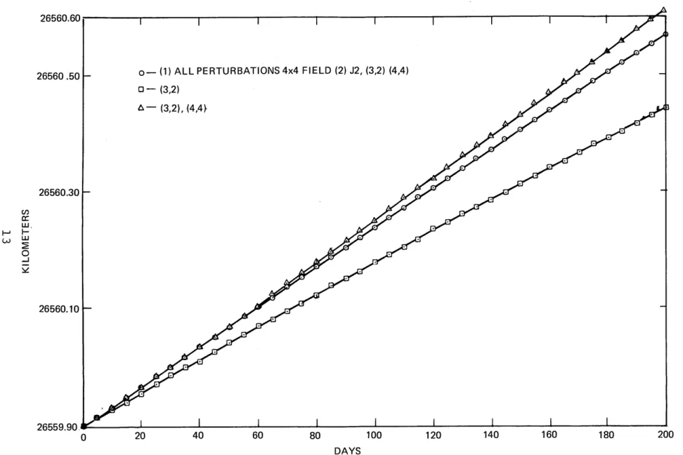
2. Semi-major Axis vs. Time for the Nominal GPS Orbit. 13

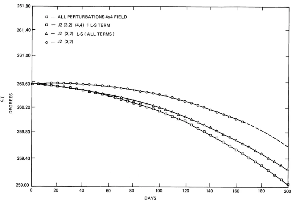
3. Geographic Longitude of Ascending Node vs. Time for 15 for the Nominal GPS Orbit.

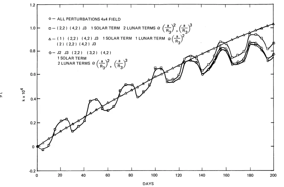
4. k = e cos (w + Q) Growth vs. Time for the Nominal 16 GPS Orbit.

5. Geographic Longitude of Ascending Node vs. Time 46

with Semi-major Axis Bias.

6. Semi-major Axis vs. Time for Different Values of 47

the Mean Longitude.

7. Semi-major Axis vs. Time for Modified Mission Orbits. 49 8. Geographic Longitude of Ascending Node vs. Time for 50

Modified Mission Orbits.

9. Long Term Semi-major Axis Growth vs. Time for 52

Modified Mission Orbits with Semi-major Axis Bias.

10. Long Term Evolution of Geographic Node Crossing vs. 53

Time for Modified Orbits with Semi-major Axis Bias.

11. Long Term Eccentricity Growth vs. Time for Modified 54

LIST OF TABLES

Table

1i. List of ESMAP Runs ...

Allowed Values of s for GPS Resonant Potential... ...

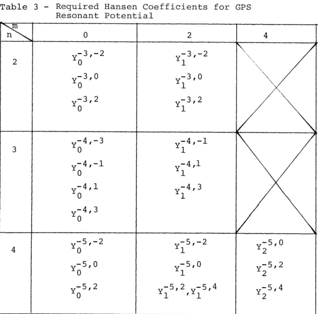
Required Hansen coefficients for GPS

Resonant Potential ...

Analytically Predicted Models...

Computational Cost of Numerical

Averaging ... ...

Comparison of Analytical with Numerical Computation of Mean Element Rates...

Stable Inclinations...

Introduction

The Global Positioning System (GPS) is a navigational system consisting of a constellation of satellites that provide continuous radio frequency coverage of the Earth. This system is designed to fulfill a need for accurate

position and velocity fixes not only for land based users, but also for users in the near-Earth environment. The transmitted satellite message contains information necessary for a user to determine his position and velocity given that he can acquire any four of the space vehicles in the constellation. This

information includes accurate representations of the vehicle ephemerides as well as time and clock corrections. The actual

fix is accomplished by measuring the range to several of the GPS satellites from which a user can reconstruct his position

in three dimensions. This is accomplished by generating a replica of the satellite signal which is shifted in time until correlation with the transmitted signal is achieved. The

time delay is then divided by the speed of light to produce the required range data. Likewise, range rate is measured to allow the computation of user velocity ( . The selected orbit

for GPS implementation is a 12 hour, low eccentricity trajectory with a repeating groundtrack which will be very closely

monitored and controlled to insure maximum mission lifetime and to facilitate user acquisition.

The requirement for stationkeeping stems from the real-ization that the satellite motion is not Keplerian (not

movement under a strictly inverse square gravitational field). If the motion were strictly Keplerian, then an initial set of orbital elements (see Appendix A for an overview of orbital elements and variation of parameters) could be chosen such

that the subsequent orbit would satisfy the mission constraints in perpetuity. However, natural perturbations resulting from the non-sphericity of the Earth, third body effects, and solar radiation pressure cause deviations from the Keplerian orbit for which corrections must periodically be applied.

Specifi-cally, the GPS mission constraints are:

(1) ±2 second deviation in the period, p(2). Since the semi-major axis, a, is connected to the mean motion, n, and the orbital period, T, through the relations

2 3 na =p n T = 27

where, p = gravitational constant,

an equivalent bound can be given in terms of the semi-major axis which can be computed from 6P for small 6P. For a

12 hour orbit, the corresponding bound on a is approximately ±822 meters. This will be used for the sake of convenience in subsequent analysis.

(2) Bound on the eccentricity of .015, with a nominal value less than .005 ( 3 ). This will allow full coverage to be

provided with the minimum number of satellites.

(3) Bound on the groundtrack that requires that the geographic node crossing stay within ±20 of the nominal value(2)

(4) Initial inclination of 63.440. This is the so-called critical inclination for which the eccentricity growth due to J3 is zero.

At this altitude, the inclination is expected to remain quite stable and will accordingly be allowed to drift without

stationkeeping (2)

This thesis will be primarily concerned with the

construction of computationally efficient, compact, reduced force models for the long-term prediction and orbital stability studies of the GPS trajectory. A corollary matter will be

to estimate the time between stationkeeping maneuvers required to maintain the mission constraints. A technical approach

with several components will guide the following presentation. A variation of parameters (VOP) formulation of the orbit

prediction problem will be substituted for a brute-force Cowell integration of the equations of motion. This is desirable

for a variety of reasons. First, VOP usually allows for the more rapid and efficient computation of the orbit when the

perturbing accelerations are much smaller than the central force term as is the case here. Second, this formulation has the advantage of being amenable to averaging of the orbital dynamics to produce equations that are computationally more

efficient. This point will now be discussed.

The unaveraged time history of the osculating orbital elements can be broken into several temporal categories, those being,

(A) short period - oscillations whose periods are less than the orbital period.

(B) medium period. (C) long period.

(D) secular - unbounded, non-periodic drifts in the elements. The short periodic variations in the elements are bounded and generally of low amplitude. In long-term orbit prediction and especially in studies which serve to establish preliminary stationkeeping guidelines, knowledge of these effects is

rendered superfluous by the much more substantial contributions in the next three categories. Their presence then serves only to increase integration time needlessly since the required step-size is dictated by the highest frequency components. In this thesis, the short periodic effects will be eliminated by averaging (to first order, over two orbits) with respect to the phase angle variable to produce a set of VOP equations in mean elements.

The last component of the technical approach has to do with the judicious selection of orbital elements in which to

express the VOP equations. The classical elements are poorly defined for inclinations of 00 and 1800 and for eccentricities near 0. The variation of parameters equations for these

elements become correspondingly intractable, both numerically and analytically in regions about these singularities. This requires inefficiently small step-sizes for their computation in numerical programs and induces non-physical oscillations in the elements. The GPS orbit does not have an inclination singularity problem, but does have a low e singularity making the pericenter very poorly defined. A change to another set of orbital elements that are well conditioned everywhere will

serve to remove this singularity from the subsequently construc-ted analytical models. A set of non-singular equinoctial

orbital elements will be employed to circumvent any numerical ill-conditioning. These are described in Appendix A.

The thesis will be divided into three main sections. Section I consists of a numerical study to determine reduced force models for the integration of the GPS variation of param-eters equations. Analytical justification for these reductions will then be presented. Of major interest here will be the

low orbital eccentricity which will be shown to cause only a mathematically prescribed subset of the gravitational field to have a significant influence on a given orbital element.

The GPS orbit has a repeating groundtrack, in part by virtue of its 2:1 commensurability with the Earth's rotation. As a result, this is a resonant orbit as well. Generally, the longitude dependent tesseral harmonics contribute rather low amplitude, short periodic oscillations which are overwhelmed by the effects of the first few zonal harmonics in

the Earth's potential. In the computation of the mean element rates these effects are largely averaged out. However,

commensurability of the satellite's period with the rotation of the Earth causes some of these terms to be amplified, the result of which is large, long period oscillations in the motion of the satellite in a way that is partially analogous

to resonance in a linear mechanical system. These resonant tesserals can no longer be ignored since they now contribute a significant portion of the vehicle's long term motion. In fact, in some ways the tesserals are the only terms that affect the relative geometry of the satellites in the constellation. Until recently, there had been no analytical representation of the tesseral potential in non-singular elements as has existed classically for some years (4 )_.

This deficiency has required a Gaussian form of the VOP equations in which the contributions of the tesserals is known only as a function

( 5)

position and velocity . Numerical averaging of the tesserals must be performed at great computational expense.

Section II will present an analytically averaged potential for the GPS resonant tesserals. On the basis of this, it will be demonstrated that highly accurate computation of the mean element rates will be possible without the need of time

consuming numerical quadrature. Appendix C presents a de-scription of the computerized symbolic algebra involved in the construction of the analytically averaged potential.

The development of simple, explicit analytical models for the averaged element rates in Section II greatly assists in the search for passive stationkeeping mechanisms since the orbital physics are now more apparent. Section III will use these expressions to construct a modified 12 hour circular orbit which meets the orbital bounds almost entirely through a passive stationkeeping mechanism. An estimate of the

required time between maneuvers necessary to maintain

the absolute and relative positions of the satellites for this scheme is compared with that required given the nominal

Section I: Reduced Force Models for GPS Orbits

In long-term prediction and stability analysis of orbits it is common practice to average the variation of parameters equations to remove short periodic components from the

orbital dynamics. This means that the non-resonant tesseral harmonics, which contribute only short period effects, can be neglected. This allows for a significant reduction in the

force models required to integrate the VOP equations. Also, since the satellite orbit for GPS will be well outside the earth's atmosphere, drag is negligible. However, integrating the averaged VOP equations forced by the remaining perturba-tions is still needlessly inefficient. As it will soon by shown numerically, with analytic justification to follow, the

low GPS eccentricity strongly decouples the perturbations in their effects on the various element rates. It does so in such a way that only a subset of those remaining will have an appreciable effect on a given element. The same property will also allow for a dramatic truncation of the lunar potential.

The numerical study must begin with a set of orbital elements at epoch. All runs in the section were made with*:

e =0 h = k = 0

M = = = 0 ; 0 = 0

o o

i = 63.440 * p = 0, q = .618

In appendix B, an expression is derived whose solution yields the semi-major axis required for a repeating ground-track, given a commensurability condition. For a 2:1

commensurability, the corresponding a = 26559.9 km. Section III, which deals with stationkeeping, will consider the effect on the long-term orbital evolution of adjusting these epoch values.

All ESMAP simulations performed with an epoch of January 1, 1980 (0 hours, 0 minutes, 0 seconds).

Numerical Approach

The numerical approach to the problem was conducted

using the Earth Satellite Mission Analysis Program (ESMAP)(6) The modified version used( 7 )

is presently resident on the Amdahl 470 at the Charles Stark Draper Laboratory. The

program computes the mean element rates in the presence of a user defined subset of a 4 x 4 geopotential field,

luni-solar effects, and atmospheric drag. The numerical attack was to select a certain subset of the full perturbation model

deemed dominant in the long-term evolution of an element. This reduced force model was used to integrate the equations of motion for a 200 day arc, the result of which was compared with a similar run using all perturbations. Those models that compared most favorably (i.e., were closest for the longest

time) were selected. A matrix of the runs is presented in Table 1.

Aiding in the selection of the models was the Harmonic (8 ) (9 )

Analysis Program , This is an implementation of first order solutions to the variation of parameters equations in classical elements. _{These solutions are based on Kaula's} formulation of the gravitational potential in classical

(4) orbital coordinates,

pRe F mp(i) G (e)S (,MR,) (1)

VPm p=0

P

m = Gpq kmpq where Smpq - m even Zmpq _cos

L(-2p)w

_{+ (£-2p+q)M + m(G-,)} Sm z - m odd + ₉ESm - -m even sin (-2p)w + (£-2p+q)M + m(Q - 6) Cm _{- m odd}

Run # Zonals Tesserals Luni-Solar Effects

S1 J2 NONE NONE

2 J₂,J₃,J₄,J₂ 4 X 4 FIELD 1 SOLAR, LUNAR TERMS THROUGH (36 2

3 J₂ J₃ 4'J2 4 X 4 FIELD, ObD ORDER 1 SOLAR,LUNAR TERMS

HARMONICS EXCLUDED a 6 THROUGH (a) R3 4 NONE (2,2) (3,2) (4,4) NONE w 5 NONE (3,2) (4,4) NONE 6 NONE (3,2) NONE 7 J2 (3,2) (4,4) NONE 8 J2 (3,2) NONE

9 J2 (3,2) 1 SOLAR TERM, LUNAR TERMS

THROUGH (a 6 3

10 J2 (3,2) (4,4) 1 SOLAR TERM, LUNAR TERMS

0 THROUGH ( 6

R

3

11 J2 (3,2) (4,4) 1 SOLAR TERM, 1 LUNAR

TERM a (R 2 3

12 J3 (2,2) (4,2) NONE

13 J3 (2,2) (4,2) 1 SOLAR TERM, 1 LUNAR

TERM a )2 R 3

az

14 J3 (2,2) (4,2) 1 SOLAR TERM, 2 LUNAR

STERMS a (R )2 () 3

15 J~ J3 (2,2) (4,2) (3,2) R ' 3 a 2 a 3

2 1 SOLAR TERM, 2 LUNAR TERMS a(R 2, (R )

3 3

Table 1. List of ESMAP Runs

e = Greenwich hour angle

R = equatorial radius of the earth

G (e) = polynomials in the eccentricity £pq

F (i) = polynomials in the cosine of the orbital inclination £.mp

p = gravitational constant

k = degree of harmonic

m = order of harmonic

The pertinent drift rate solutions are given by (4)

R 2F mpG pq (k - 2p + q)SZmp mmpq e nmp Aampq =Re I na + 2 (£-2p)) + (Z-2p+q)M + m(Q - 6) SF1mpGpq(e2/ 2 1/2 SFmpGpq(l-e2 1-e 2 (-2p+q)- (-2p) Smpq Ae =mpq =Re _k+3 na _{e&E-2p)A + (£-2p+q)M + m( - 0)6}

Ak mpq = pRe

(3

F ,mp/i) G EpqS mpq

na+3 (1-e2)1/2sin i E -2p)j + (k-2p+q)M + m(i-)

S mpq is defined as the integral of Simpq with respect to its argument. HAP seeks to identify the resonant tesserals and computes their contributions to the evolution of the orbital elements given epoch values of a, e, and i. The program suffers however from a zero eccentricity singularity in the solution for the eccentricity drift. Thus, the

nominal epoch value of 0 for the GPS eccentricity was not used. The actual epoch values input to the program were

a = 4.164 Earth radii = 26558.57 km

e = .001

i = 63.440

The resonant tesserals selected by the program were taken as good initial guesses for the construction of the reduced models. One interesting point is that no odd order

(m = odd) tesserals are among those listed. This indicates that the odd order harmonics contribute only short period effects which would be filtered out of the long-term dynamics by the numerical quadrature. On this basis, the odd order harmonics were deleted from the models in a first step at reduction.

Inspection of the HAP output in Figure 1 gives an idea of what harmonics will dominate by degree L and order M. The node crossing rate (D [NODE] ) is determined primarily by (3, 2) and (4, 4) with all other contributions at least an order of magnitude less. This is also true of the semi-major axis rate (D [A] column). The eccentricity growth, on the other hand, is dominated by (2, 2) and (4, 2) (D [E column). This served as a basis for constructing the tesseral portion of the reduced models. The major zonals were then included and their effects weighed. The lunar potential has factors in the expansion which are of the form( 3 n where R

is the Earth-moon distance. This ratio is small, so that an attempt was made to truncate the potential to at most two terms.

SATELLITE 12HLU

SEIT DEPIOD =6232.5 DAYS

-- RESCNANT PERTUREATIONS

PRIMARY RESONANCE WITH TEPMS OF ORDER 2

A= 4.1A4 E.R9. r=-. of% I--I= 6?.&& DEG. L M r0 I ' (DAYS) 0( A) (M) M DOT = 722.086 DEC/CAY

i DCT ^ 330 £EC'0'PY E01EV IlGHT - 2150 p 5KM

NODE DCT= -0.033 CEG/DAY PERIOD = 11.965 HCURS

O(E 0 I) D (____( M)

(DEG) (DEG) (DEG)

APOGEE HEIGHT F 0.2321D 05 KM

ORBITAL FREQ. = 2.016 C/DAY

VELOCITY_ CCMP. C w/SEC)

RADIAL TRANS. NORMAL

(NOOEJ_ POSITION COMPONENTS (M) (DEG) RADIAL TRANS. NORMAL

S2 P"P -!F,33929- 7-21D '1 1.36D- 9.f40 06-.-:.09 01 .110) 01 2.30-94 3.70- OA 1. 03 5.5D 01 5.4 02 5.7D :! 4.60- -0 2 2 2 1 1631.l5 1.96D 02 3.120-03-4.000-04 1.790 02-1.86D 02 5.31D-05 8.50 04 -3.AD 03 1.5D 02 1.2D 03 1.3D )j 1.90 00 2

3 2 1 1032.71-6.310 03 4.060-Oe 8.C70-33-5.720-02 1.85D 02 3.230-02 6.10 04 9.1D 34 170, 04 8.90 02 9.40-1) 3.9D 01 2

= -2

9 7 -1 33 .991 .6b0- Ot-If-1,2-lU -de -07 7.1iT --0 0-u 0ov -e4V02 -D2 I5 --eD0-7 3 6a 0Z- 4. -2- O0 45

4 2 2 15"31.'1-1.03D 00-1.950-35 2.490-06-1.110 00 1.16D 00 1.710-05 5.30 02 2.30 01 6.8D 00 7.7D 00 8.10-0j 1.20-02 2

I4 1 0331e.23 1.91D 03-1.830-08-3.580-03 6.640-03-4.110 01 1.750-03 1.40 04 -4.00 04 1.2D 03 2.CD 02 4.20-31 1.7D 31 3 5 2 2 06632.471-1.140 02 1.64D-09 3.250-04-3.47D-03 7.480 00-1.370-04 2.50 33 3.70 03 2.40 02 3.60 01 3.80-34 1.60 00 2

1

, 2 ? ::40 01 700D-0I- -0 O- C- .. 0'0 1 4.17-31- 9.-90-07 10.9 '2 1.60 01 7.30 q 2.-9 o0 -R-9 44 7.60 903 2 6 2 3 l6631.ns-9. AD-02-1.81D-06 2.32D-07-1.04D-01 1.080-01 3.180-07 A.90 '1 2.10 00 1.20-31 7.20-01 7.6D-3. I.1D-3- 2 6 & 2 13316.236 2.79D 01-2.60C-10-5.180-05 2.380-04-5.950-01 7.540-35 2.00 02 -5.EC 02 2.60 01 2.80 00 6.00-34 2.50-01 2 6 6 2 1221'.62 2.21D-01 1.38D-06-4.53D-C7 7.930-02-8.250-02 1.530-07 3.80 01 -4.50 00 1.50-01 .30-01 1.70-3) 2.20-03 2 7 2 3 -0532.471- 6.150 ( 60 -oD-11 7*77D-16-1280-04 1*790-01 -2 63D-05 59D0 1 87) 01I . 70 00 0. 50- 900- 3.70- 02 7 6 2 0221'.e24-5.76D-01 5.420-12 1.C80-06-8.00D-06 8.270-03 1.08D-05 2.80 30 1.2C 01 4.70 00 4.00-02 1.3D-3 , 5.20-03 2 8 LL 3 0316.236 2.39D-01-2.25D-12-4.480-07 2.530-06-5.150-03 3.920-06 1.7D 30 -5.30 00 1.50 03 2.50-02 5.2D-)~ 2.10-03 2 9 E 3 0221m.824-1.05D-01 9.910-12 1.970-07-1.36C-06 1.510-03 3.120-07 5.10-31 2.20 00 1.70-01 7.2D-03 2.30- . 9.40-04 2 PMS eEAT PERIOD FOo L)16=

RMW AAPLITUDE FOQ 0Q= QM5 A DMLITUDE FOP O) 0 0.5C82490 04 0-24 6110 15 0.33131670 05 C.14042710 CA 8SS AMDLITLDES 0=0 TO 0) Q 9PS AMPLITUDE RSS AMPLITUDE FSS AMPLITUDE 26.753 0-994644D __ _ _ 0.99395010 05 0.37153510 04

The selected set of reduced models that resulted is:

Figure 2 clearly shows that by far the most important contribution to the semi-major axis rate is the resonant tesseral (3,2). This observation is used in Section III to develop a passive stationkeeping procedure that can be

implemented choosing epoch elements based on nulling just

a(3,2). The addition of (4,4) produces a model that is much closer to the all perturbations run, however there remains a discrepancy that results in a divergence of 50 meters after

Element rate Model Illustration

(3,2) , (4,4) , J2 Figure 2

(3,2) , (4,4) , J2, Figure 3

solar point mass term, 1 lunar term a )2

(2,2), (3,2), (4,2) J3, Figure 4 J2' 2 lunar terms a

26560.1 26560 .50 26560.30 en C 0 26560.10 26559.90 I I I I I I I 0 20 40 60 80 100 120 140 160 180 DAYS 200

Figure 2. Semi-major Axis (km) vs.Time for the Nominal GPS Orbit __~-~

--L1---200 days. The inclusion of the J2 zonal eliminates the discrepancy and completes a model which is virtually

indistinguishable from the full force representation. The presence of J2 is surprising since mathematically, the semi-major axis rate due to this harmonic is 0. The observed effect is a resonance phenomenon and is caused by the

influence of J2 perturbation on the mean longitude coupling into the a rate.

The geocentric longitude of the ascending node is controlled by the same geopotential harmonics as the semi-major axis. As previously stated, there is in fact consider-able coupling between the two. In Figure 3 it is seen that a J2, (3,2) model constitutes a significant portion of the perturbed motion. The addition of the full lunar potential

(through (a/R₃) ) produces much closer agreement, but exposes the need to introduce (4,4). A truncation of the lunar

potential in the final model was possible by including only one term, proportional to (a/R3)2 , with nearly no degradation. Evidently contributions from higher order terms are

essentially negligible.

Figure 4 shows the k component of the eccentricity since some of the more interesting variations were found here. A

model containing J3, (2,2), and (4,2) produced the major portion of the growth. Inclusion of a lunar potential term proportional

to ( )2 in an attempt to model the medium period oscillation apparent in the all perturbations run, had virtually no

effect, a rather intuitively surprising result. Adding the next term ((a/R 3) 3), however, yielded the desired evolution with all other terms contributing much less. The divergence between this model and the full field model is due to the

same resonance phenomena observed in the semi-major axis rate. Since the mean longitude is coupled into the eccentricity it must be properly modelled as well. Therefore the addition of J2 and (3,2) to the final model to correct for errors in the

0 20 40 60 80 100 120 140 160 180 200 DAYS

Figure 3. Geographic Longitude of Ascending Node ( Deg ) vs. TIME for the Nominal GPS Orbit 261.80 LU Ln iii , U w w 03 ~_~ ~II ___

---20 40 60 80 100 120 140 160 180

DAYS

Figure 4. k = e Cos (W+ Q) _{Growth vs. Time ( Days ) for the Nominal GPS Orbit}

1.0 0.8 0.6 0.2 0 -0.2 200 ~3-T~- L -r)--Y- --- - -~ ~-- -- 7---_ _---- --- --;- -L----s~-~

----mean longitude, results in excellent agreement with "ALL PERTS."*

All of the reduced models are suitable for judging the long-term stability of the GPS orbit. They are also found to be excellent replacements for full force

representations over long time spans and may be used to integrate the averaged VOP equations with good results.

One is reminded that the "ALL PERTS" run is in all cases the full field of ESMAP perturbations, exclusive of the odd order tesseral harmonics.

Analytical Approach

The observed decoupling between the geopotential

harmonics in their effects on the mean element rates can be justified on analytical grounds. Likewise, the neglect of terms in the lunar potential is mathematically justifiable. Each of these will now be considered in detail.

The basic expansion for the geopotential comes from a solution of Laplace's equation, V2_{U = 0, in spherical}

coordinates and is given by(4)

U I N = " nm nm + nm

U

_{r n=2 m=0}

a

_r

where, p = gravitational constant = G(m _e + m _s ) m = mass of satellite

s

m = mass of Earth e

r = distance from Earth to satellite R = equatorial radius of the Earth

= geocentric latitude

X = geographic longitude of the satellite

Pnm (sin p) = associated Legendre function of degree, n, and order, m

Cnm, S = empirically determined gravity harmonic coefficients

The terms in this expansion for which m = 0 are called zonal harmonics and arise due to the nonsphericity of the Earth along a meridian. Accordingly, they possess symmetry about the Earth's rotation axis. The terms for which m 0 are called tesseral harmonics and represent the longitudinally

dependent deviations from sphericity.

As will be demonstrated more thoroughly in Section II, it is desirable to have the potential expressed directly in orbital elements. In implementing the Variation of Para-meters equations this circumvents the computationally costly coordinate transformations otherwise required and allows for analytical averaging to remove short period components. An algebraic conversion of the spherical harmonic disturbing potential, (2), to classical elements has been available due to Kaula for several years, (1). A similar expression in

the non-singular elements needed for GPS analysis has only recently been developed and for a general harmonic is the real part of (10) Rn , n SCnm Vm S(pq) (3) nm a \a /n,s Cnm _s=-n 2n +C0 X Y

t-n-l,s(k,h)

exp

j(t

X - mO t=-_0

where, a = satellite orbit semi-major axis Cnm= Cnm jS ; j =

nm* nm - nm

X = mean longitude M + w + Q 0 = Greenwich hour angle

S(m,s) (p,q) is a special function, related to the Jacobi 2n

polynomials P (U,) that contains the equinoctial elements

n

p and q which orient the orbital frame with respect to inertial space. The S function arises from the rotation of the

spherical harmonics in (2) into the orbital reference frame. They are computed according to the following rules

m-r (l+p 2+q2 )-(p+jq) r-m (r-m,r+m) (Y) r n-r (m,r) (n+m)(n-m)! + 2 +2 -m m-r (m-r,r+m) 2n (n+r)!(n-r) n--m -m < r < + (+p2 +q2 r (pjq)m-r (m-r,-m-r) y) r < - m +p+q (pjq) () r <- m n+r (4) > m (Y) where, 2 2 S= (1-p 2-q = cos i (l+p 2+q 2 dn n dx

The expression of the form Y 'Y (k,h) is another special

function in the eccentricity analogs h and k, closely related to the standard Hansen coefficients, X , (e).

0a n,m = (k+jh)m-t n,-m 2 +k2 ) t G +m-t, n,m = (k-jh)t-m n,m (h2+k 2) n (k-jh) XU+tm (h t E +t-m,=0 o=O t < m (5) t > m (-) n2nn' (l-x) (l+x) B m r (l- (,+X) (l-x2) P ( , ) (x)_n

where,

X - constant Newcomb operators

(see Appendix C) Last of all, Vm (n-s) ' n,s (n-m)! P n,s (0) ds where, P (0) -n,s dv P n (v) v = 0 P (0) = (-1) (n-s) P (0) n,-s (n+s)! n,s

P (v) = Legendre polynomial of order, n n

The preliminary simplification of (3) is begun by re-calling that the GPS orbit is resonant due to the 2:1

commensurability with the Earth's rotation. In general, the averaged elements of the orbit will be influenced by terms in the geopotential for which the trigonometric argument of (3) is slowly varying, or mathematically started, terms for which

t X - m 80 0 (7)

t = m&

(6)

But e/X is equal to 1/2 so that equation (8) becomes

t m ₂ (9)

Now if m/2 is not an integer, then a harmonic of order m cannot contribute to the resonant potential . One immediately notes that all odd order harmonics are non-resonant. Consequently, they contribute short periodic oscillations which can be

neglected for long-term averaged orbit studies. This result

is consistent with the numerical section. (9) allows the resonant potential to be expressed as

U _nm - _a R _a C _nm exp

j

m (X -₂ 20 (10)

nE ₅ (m,s) -n-l,s

X V _{n,s 2n} ms) (p,q) Y _m (k,h )

s=-n 2

Since ( e) is approximately .24, further truncation of (10) a

is effected by eliminating terms associated with powers of this ratio greater than four. Thus, the full resonant potential can now be expressed as the real part of

4 -n n m S- a 4 C nm exp i(X-2e6 (11) n=2 m=0 n n XE V m S(ms) (pq) y-n-l,s (k,h) s-n n,s 2n m m = 0, 2, 4

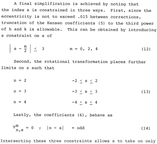
A final simplification is achieved by noting that

the index s is constrained in three ways. First, since the eccentricity is not to exceed .015 between corrections,

truncation of the Hansen coefficients (5) to the third power of h and k is allowable. This can be obtained by introducing

a constraint on s of m

s < 3

2 - m = 0, 2, 4

Second, the rotational transformation places further limits on s such that

n = 2 n = 3 n = 4 -2 < s < 2 -3 < s < 3 -4 < s < 4 (13)

Lastly, the coefficients (6), behave as

Vm _{= 0}

n,s In - sI = odd (14)

Intersecting these three constraints allows s to take on only the values displayed in Table 2.

Table 2 - _{Allowed Values of s for GPS Resonant Potential}

n m s 2 0 -2, 0, 2 2 -2, 0, 2 0 -3, -1, 1,3 1 _{-1, 1, 3} 0 -2, 0, 2 4 2 -2, 0, 2,4 4 0, 2, 4 (12)

An array of harmonics with their associated Hansen

coefficients can now be constructed and is given in Table 3.

Table 3 - Required Hansen Coefficients for Resonant Potential GPS rnm 0 2 4 -3,-2 Y-3,-2 -3,0 -3,0 Y Y 0 1 -3,2 -3,2 0 1 -4,-3 -4,-1 3 0 Y1 -4,-1 -4,1 0 1 -4,1 -4,3 0 1 -4,3 Y 0 -5,-2 -5,-2 -5,0 4 0 1 2 -5,0 -5,0 -5,2 0 1 2 -5,2 -5,2 -5,4 -5,4 0 1 1 2

From this array and the definition of the modified Hansen coefficients, (5), the resonant potential can be written term by term:

+0 (02) -3

2,2 4 0

2

(e

(a

)

2 -3, -2 = (k-jh) X2 -2 2,0 (h + k2 ) 2 -3,-2 (k + jh) X 2_2,00 C 2 2 2 (2,0) 2,0 4 -3,0 + 2 1 2,2 4 where (k-jh) X ' 3,0 (k-jh)

LX3,0

Ixi f (k+jh) ir2 E 1,0 R e) 30 a 30 [ 3,-3 6 -3,0 2,1 (h2 -3,-2 2,1 0,-3) -4,-3 0 + k2) (h2 + k2J + 0 (0,-1) -4 -1 + -i 6 ' (17) 3,-1 6 0 + (0,1) -4, + 0 (03) -4,3 3,l 6 0 3,3 6 0 where -Y3, - 2 0 -3,0 Y -3,2 Y₀ U* -2 -2 a (16) (2,2) -3,2] -3,-2 Y 1 -3,0 1 -3,2 1 U 3 0 -a

-3,0

x-3,0

X + X 0,0 1,l S(2,-2) -3,-2 S Y 4 1 E1 - 2 2 -2 e ] 2,-2

3 -4,-3 = (k - jh) X)' 3,0 (k - jh) 4f,-' 1,f = (k + jh) = (k + jh) 14 -1 -4,-1 2,₁ -4,-1 + X 1 2,1 -4,-1 Y -4,1 Y -4,3 Yo 0 3

e

)

(a

C323 2

e

j

e-21

_{32_,-1}

(18) 2 + V₃ 3,3 where

(2,3)

- 4,

S Y 6 1 2 -4 -1 = (k - jh) 2 X-4,-2,0 Y-41 -4,+ -4 ,1 1 0,0 1,1 = (k + jh)2 -4, -3 2,0 where -4,-3 YO -4,-3 3,0 (h2 (h2 + k 2 + k 2j) 32 U3 2 _a 2 (2,1) -4,1 3,1 6 1 -4,-1 1 (h2 + k2 ) -4 1 $6(2,-1) Y 4,-11 S Y 6 1

s8 (0-2) -5,-2 + v4 0 8 0 4,0 + S 4,2 where Y0-5, - 2 0 (0,2) y -5,2] 8 = (k - jh) 2 X-5,-2 2,0 -5,0 -5,0 0 0,0 +-5,0 + i 1,l (h 2 = (k + jh) 2 -5,-2 2,0

4R

)

Ra C* e j _-2ev 2 42 4-2 2 (2,0) -5,0 + V S Y 4,0 8 1 2 + V 4,2 (2,2) -5,2 S Y 8 1 + 2 (24) -5 4,4 8 1 where -5,-2 Y1 -5,0 1 -5,2 1 -5,4 1 S(k - jh) X-5-2 = (k - jh) = (k + jh) 520 -5,0 + X 1 2, -5,-2 + X 2,1 (k + jh) -5,-4 3,0 * ' p 4 0 -40 a 4 Ce) 4 a 40 V 0 4,-2 (19) (0,0) -5,0 S Y 8 0 + k2₎ -5,2 Y0₀ U* -4 2 a (2,-2) 8 (20) (h2 + k2) (h2 + k 2

*

P

c

e

2 2 ₄

₀

_{, (}4

_,0)

_-5,0(2

U ₄₄ -_-a C ₄₄ e _{,0 8} (21) 2 + V4 S(42) -5,2 + 4 (4 ,4 ) -5,4 4,2 8 2 4,4 8 2 where

-5,0

2

-5,0

Y250 (k - jh)2 X2,0 -5,2 -5-2 -5 -2 2 2 Y2 ₂ = X ,0 + X (h + k ) 0,0 1,l Y24 (k + jh)2 X2,05 4

It is notable that some harmonics have associated Hansen coefficients which contain only even powers of the eccentricity, while others contain only odd powers. In general one finds,

for the GPS orbit, that harmonics for which n - m/2 is even, are dependent only on the even powers of h and k. Similarly

for n - m/2 odd, only odd powers appear.

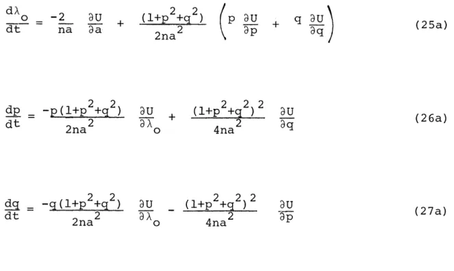
Now, it is possible to tell how the resonant harmonics decouple in the element rates by inspection. To do this, a set of low eccentricity equinoctial VOP equations is presented

for which powers of h and k greater than 1 have been neglected

da 2 U

dt na a (22)

o

dh _ 1

/

U h U k(l+p 2+q 2) pU + q

dk _ 1 a + k2 2 dk _ 1 U k U h(l+p2+q2 ) dt na2 -h 2 f ) 2na na o2na

p

a-

+

p dX _ 2 U + dt na Da 1 _{h U +} 2na2 ( -h + 2na _k ) ₊ (1+p +q 2) p DU U 2na2 ap ag (25) dp _ -p(l+p2 +q2 ) k _U dt 2na2

)

h h U 3 + 8k

U \

3x 0) (l+p 2+q 2) 2 U (26) 4na 2 2 dq _ -q(l+p2+q2 ( ) k U dt 2na2

)

h h _U + DU ak a 2 2 2 (l+p +q ) 2 U 2 4p 4na

The procedure is a simple matter of selecting as dominant, in a particular element rate, those harmonics that contribute terms in the 0t h power of h and k. To facilitate the analysis all terms in (22) - (27) that have factors of h and k, will be neglected since they contain powers of the eccentricity of no

less than one. The VOP equations can now be written as

da 2 DU dt na UX 0 dh _1 U dt 2 Tk na dk 1 DU dt 2 3h na (22a) (23a) (24a) qU q 3 (24) (27)

od -2 9U (l+p 2+q ) _{p U} q U dt na 9a 2na2 9qp q 22 g2 2 2 dp -p(l+p +q ) U + +p +q2) 2 U dt 2na o 4na2 2 2 2 2 2 dg = -q(l+p +q ) DU (l+p +q ) 2 U dt 2 a 2 p 2na o 4na (25a) (26a) (27a)

Now, in those rates whose remaining terms have no derivatives with respect to h and k, potential harmonics that contain

th

0 powers of h and k will dominate (n-m/2 even). In cases where derivatives of h and k appear, harmonics that contain

1st powers of h and k will dominate (n-m/2 odd). A quick check yields Table 4.

Table 4 - Analytically Predicted Models

Element rate Dominant Harmonics

A J 2 ,J 4 ,(3,2), (4,4) h J3, (2,2), (4,2) k J₃, (2,2), (4,2) 0Xo J2' J4' (3,2), (4,4) J2 ' J4' (3,2), (4,4) eJ2' J4' (3,2), (4,4)

The table is readily extended using the parity of n-m/2 as a guide. This decoupling is exactly that demonstrated in the numerical study performed by ESMAP. It is necessary to realize that the observed harmonic decoupling is not

generally valid. However, in the case of the GPS orbit, the near zero eccentricity has caused this to happen. Support for this contention comes from a consideration of the Soviet

Molniya communications satellites which move in highly eccentric (~.74), 12 hour orbits at the critical inclination of nearly 650. These satellites have partially stabilized groundtracks which give rise to resonance as for GPS. However, it is found

that the dominant harmonic affecting period change and nodal drift is (2,2) rather than (3,2). In fact the transition between (3,2) dominance and (2,2) control of the semi-major

axis appears to be an eccentricity of approximately .05(11) In the numerical section, terms of the lunar potential were required to adequately model the nodal drift and

eccen-tricity growth. This was especially evident in the case of the eccentricity where the exclusion of the (3) 3 term would have resulted in the failure to model a significant medium period oscillation. The result was surprising since we might have expected the 3 2 term to exert the dominant influence. An analytical approach is possible to explain the phenomenon as well as show which terms, if any, of the lunar potential will dominate in their effect on the other element rates.

To illustrate, the lunar potential is given by(1 2 )

F(L) L n=2 ) P (cos i) (28)

L n=2 RL n

where, PL = lunar gravitational constant R_L = earth-moon distance

r = earth-satellite distance = angle between r and R

S -L

P (cos i) = nth Legendre polynomial

The corresponding averaged potential of interest here can be written, after multiplying by (a/a) n, as(12)

(L) _{- RL n=22} L (an 1 rn

Pn(cos p) dX (29)

R n=2 RL 2o a n

where, X = mean longitude - M + w + 0

Now (cos p) can be rewritten in terms of the true longitude,

L(=f + w + Q, f = true anomaly), as

cos = al a cos L + B₁ sin L (30) where, al' ₁ - direction cosines of the moon relative

to the equinoctial orbital frame.

It is well known that powers and products of trigonmetric

functions in an argument can be rewritten as the same functions containing multiples of that argument. Thus the Legendre

polynomials can be expressed in terms of even multiples of L if n is even and odd multiples if n is odd. The first two are(12):

P₂ (cos i) = S₂ + S₃ cos 2L + 3S₁ sin 2L - 1 (31)

1 5 5

P₃ (cos ) a l 4 cos 3L - B₁ S sin 3L (32)

+ 3al₁ S₂ - 1 cos L + 3 ₁ S2 - 1 sin L where

In general an even order Legendre function will contain the arguments nL, (n-2)L ... OL while an odd order

function will contain nL, (n-2)L ... lL. This

transfor-mation allows (29) to be rewritten in terms of sin NL and cos NL which is especially convenient since the averaging integrals

can now be solved via the zeroth order, modified Hansen coefficient(10)

Yn,m -1 ( r)n

YO =

7f

a

0

exp(jmL) dX ₍₃₃₎

A list of the first few integrals is(12)

P2 (cos P3 (cos ): 1 0 1 ₂ 27r 1(2 Tr 1 22rr7r

1

2iJ

f

2 Tr f 0

2

r )2 a (r _a)2 r

a)

3 2 2 dX = 1 + (h + k 2 (34) 5 2 2 cos 2LdX - (k - h sin 2LdX = 5hk 35 2 2 cos 3LdX - k(3h - k ) 8 35 2 sin 3LdX - h(h -8 (35) 2 3k ) 5 3(h 2 2 cos LdA = - k (h + k ) + (r sin LdX- h (h + k) + 1 a 2 4]

Generalizing one finds that for n even in eq. (29) even powers of the eccentricity result and for n odd, odd powers result.

Continuing, one notices that for h = k%0O, as in the GPS case, the dominant contributions to the VOP equations

for h and k are

dh ,. 1 F (36) dt _na2 -k dk

-

1 F ( (37) dt 2 9h na

After differentiation, terms in the lunar potential for which powers of h and k are even will yield at least first powers of the eccentricity. On the other hand, terms in the potential which contained odd powers may yield 0th power

contributions to the h and k element rates. Following this reasoning for very low eccentricity

dk dh ₍₃₈₎ dt dt 2 2 dh _L a -5 1 (39) dt RL L na t R L n 2 (40)

The result is consistent with the inability to model a medium period oscillation in h and k by the first term

in the lunar potential. Thus it has been demonstrated that the second term a )3 dominates due to the low GPS

(RL

eccentricity. All higher order terms contribute negligible effects since they contain correspondingly higher powers of the ratio (a)

This type of analysis can be extended to the other elements treated in the numerical study. Eliminating all

terms for which first or higher powers of h and k will be present, the rate dXo/dt can be stated as

oX 2 aF

S 2 F (41)

dt na 5a

No differentiation with respect to h and k is indicated so that only terms in the lunar potential for which there are ₀th

powers of the eccentricity will exert any appreciable

influence. Here only a )2 will have a significant effect on RL

the mean rate for X as shown in the numerical study.

The model for the semi-major axis shows that no lunar terms are required to achieve good agreement with an all perturbations run. The correct expression for this rate is

da 2 F (42)

dt na Da

However, since there is no explicit dependence of the averaged lunar potential on A for any power of a the rate is zero, as expected.

Thus analytical justification can be found for the select-ion of the reduced force models for GPS, largely on the basis of the extremely low nominal eccentricity.

Section II A New Method for Treating Resonant Tesserals

The inclusion of resonant tesserals in long-term orbit prediction has, until recently, presented a real problem. The efficient computation of tesseral resonance effects has been hindered by the absence of an analytical expression for

the disturbing potential in non-singular elements. This necessitated the use of the Gaussian formulation of the VOP equations in conjunction with a numerical quadrature process.

In the Gaussian formulation, the element rates are expressed in terms of the distrubing acceleration via(12)

a. a. - _

1

_

i = 1,..6 (43)

where,

Q = tesseral disturbing acceleration

a.t

ai _{partial of the i}t h

element with respect to velocity.

The disturbing acceleration is given by

(r 9r tU Q(t) (12) T T

U

p +

U

/

a

+ DU + D X (44)

where, r = position vector of the satellite in the coordina'te frame of the acceleration vector

The indicated partials are computed from(1 2) U _ _P r 2 r n=2 co (n + 1) (a = S nmsin mX + Cnm cos mlPnmP (sin )

U _ a ) mp (sin ) S cos mX - C sin ml

r r nm nm nm n=2 m=0 O C DP (sin q)

DU

- P

E

(a ) :S sin mX + C cos m nm S r n=2 r m= nm nm (45) (46) (47)

There is considerable overhead entailed in the numerical implementation of this method. As coded in ESMAP, each

evaluation of the Gaussian VOP equations [Eq. (43)] the following manipulations:

requires

(a) The computation of the partials of the equinoctial elements with respect to velocity, Da. (6)

(b) A transformation of spacecraft coordinates from the mean of 1950 to body (Earth) fixed coordinates(6)

(c) The computation of spherical coordinates, (r,X,4), from the rectangular, (x,y,z), coordinates of the body fixed system. (6)

(d) Calculation of the partials of the potential with respect to the coordinates (r,X,q) from (45) - (47)(6)

(e) A transformation of these partials in spherical coordinates back into rectangular body-fixed coordinates according to(6) U _ x U xz BU y aU r / 2 2 _{x +y} x+y BU _ay _ y _{r ar} U ₂ yz 2U _{x 2} x _{2 a} x +y au z au

₊

x +y aU (50) az r r _r2 ap

(f) A transformation of acceleration vector components to the mean of 1950 coordinate system after which the element rates are computed from equation (43)

This overhead is now multiplied since a numerical

process is used to obtain the averaged element rates. Math-ematically, this numerical process is specified by(6)

F -NT + 2r. N

n 0 1

a - 2 E n A (F) dF (51)

2 =1 F -NTr+(i-1)27rN n

N = number of orbits to be averaged over F = eccentric longitude H E + Q + w

E = eccentric anomaly

A (F) = high precision element rate computed

using Eq. (43)

n = number of quadratures used

The procedure used to evaluate this integral is to fit the integrand in Eq. (51) to an orthogonal polynomial in the eccentric longitude over N/n orbits. The integral of the orthogonal polynomial can be evaluated analytically. This method of computing integrals is known as numerical quadrature

and is required when the integrand does not exist as a tractable analytic function of the integration variable. Considerable overhead is incurred, the extent of which is

determined by the highest specified power of the interpolating polynomial. As shown in Table 5, the computation time entailed

in computing the averaged orbital element rates is greatly increased through the inclusion of the numerical quadrature for resonant tesseral harmonics.

Table 5 - Computational Cost of Numerical Averaging

Test Case Time, CPU ( ) - (1)

Centi-seconds

(1) Reference

All zonals, All luni-solar terms, 314 0

no tesserals (2)

th

1 2 order quadrature, 2 orbits 2020 1706

tesserals included (3)

2 4th order quadrature, 2 orbits 3735 3421 tesserals included

The computation time is greatly increased when the tesseral harmonics are added to the perturbation field and goes up in direct relation to the quadrature order. If one subtracts the reference run from each of the other two

assuming that what is left can be attributed to computation of th

the tesserals, it is seen that the 24 order quadrature case is almost exactly twice as costly to run as the 12th order case. Clearly, elimination of the averaging quadrature would

greatly facilitate the rapid calculation of the tesseral resonance contributions to the element histories.

As mentioned in Section I, a way to circumvent this

problem classically has been available due to Kaula for several years (1). This contribution has seen widespread use, but is of limited utility in the study of low eccentricity GPS type orbits.

However, recent results also stated in the first section, now allow for the construction of analytically averaged,

explicit VOP equations in non-singular elements. The low eccentricity of the GPS orbit facilitates the rather radical truncation of the final expressions with respect to h and k to yield Variation of Parameters equations with terms

containing powers of the eccentricity no greater than one. This form of analytical averaging removes short periodic terms and resonant terms proportional to high powers of e. The rates for (2,2), (3,2), (4,2) and (4,4) can be found in Appendix C along with the computerized algebra involved in this deriv-ation.

Using the debug option of ESMAP ( the element rates generated by the numerical averaged orbit prediction were compared with those produced by the new explicit formulae. The test cases run were

Case 1 Case 2 h= 0 h =0 e = 0 le = .01 k = 0 k = .01 .01 p = 0 p = 0 q = .618095 q = .618095 X= 0 X= 0 a = 26559.9 km a = 26559.9 km 6 = 1.73553625 radians 6 = 1.73553625 radians

The Greenwich hour angle is based on an epoch date of

January 1, 1980. A matrix of the results is seen in Table 6. The mean longitude rates are not included in this table.

The difference of several orders of magnitude between the mean motion and the contributions to the mean longitude rate due

to perturbations limited the utility of this comparison.

Agreement is generally quite close,with the rates due to (3,2) dominating where expected. It will be noticed in the zero eccentricity case, that the ESMAP runs produce small non-zero rates when zero is predicted by the explicit formulation.

Inspection of the expressions in Section 1 and Appendix C will verify that this discrepancy is not due to truncation on the eccentricity and that the prediction of zero is indeed correct. Rather,the difference is taken to be due largely to quadrature noise involved in the ESMAP numerical average. When the rates are extremely small as in the case of (4,2) and (4,4), it

is expected that the apparent deviations can be attributed in greatest part to errors in the quadrature. Remaining discrepancies are probably due to uncertainty in the

calcu-lation of the correct Greenwich hour angle at epoch.

The quite close agreement of the explicit formulation of the averaged orbital element rates with the ESMAP numerical

A = ESMAP NUMERICAL AVERAGING*

B = EXPLICIT ANALYTICALLY AVERAGED THEORY

(2,2) _{(3,2) (4,2) (4,4)} A -. 52665524xl0-1 0 .32655463xl0- 7 .67463011x10-1 1 .64613481x1-0 B 0.00 .32663116xl0- 7 0.00 .64369884xl0-8 A -. 15124436x10-10 -. 18350001x0 - 1 5 .77901248x0-1 4 .19364701x10- 1 4 B -. 15105023xl0-10 0.00 .78079905xl0- 1 4 0.00 A .72077044xl0-11 .16154185x10-14 .30750092x10-1 2 .66049711x10- 1 5 B .72294856X10-11 0.00 .30180676x10- 1 2 0.00 A -. 36835041x10-14 -. 86728999xl0- 1 2 -. 29027992x10- 1 6 .24183411xl0- 1 3 B 0.00 -. 867415332x10- 1 2 0.00 .235731083xl0-13 A -. 19563118x10- 1 5 B 0.00 -. 74039139x10- 1 2 -. 73767031xl0- 1 2 .6533585xl0-16 0.00 -. 14570422xl0- 1 2 -. 14537423x10- 1 2 A .13955590x10-8 .32674893x10- 7 .55937390x10- 1 0 .64651533x10- 8 B .15073953xl0 8 .32663116x0-7 .35297236x0-10 .64369884x10-8 A -. 15135507xl0- 1 0 .746150032x10- 1 4 .73980128xl0- 1 4 -. 96582411x10- 1 4 -10 -14 14 -13 B -. 15105023x10 .82641452x10- 1 4 .953004264x10- 1 4 -.118882411x0-13 A .72077418x10-1 1 .50586221x10- 1 3 .31031528x10-12 .32055724x10- 1 4 k .72294856x10-l .47746979x0-1 3 .300775915x0-12 .24697801xl0- 1 5 .01 A -. 28841727x0-1 2 -. 86746704xl0- 1 2 -. 21144907x10-14 .24177542x10-1 3 12 12 -14 -13 B -. 28491258x10 1 2 -. 867415332x0-1 2 -. 21239864x0-1 4 .235731083x10-13 A -. 58693955x10-1 3 -. 74096397xl0-12 -. 16580821x10-1 4 -. 14576559xl0-1 2 B -. 59016852xI0-13 -. 73745325x10-12 -. 18361513x104 -. 14536L094x102

Table 6. Comparison of Analytical with Numerical Computation of Mean Element Rates.

ESMAP Quadrature: 24th order Gaussian quadrature

2 orbital periods in averaging interval

method, as seen in Table 6, is very interesting. It

represents the first numerical verification of the assump-tions and consequent algebra involved in the construction of an analytically averaged potential for the tesseral harmonics in non-singular elements, and, as such, is quite valuable.

Several major advantages come from the existence of explicit, analytically averaged element rates. First, the computational overhead incurred by the use of the Gaussian formulation of VOP is completely eliminated. Since numerical quadrature was seen to be the primary determinant of CPU time it is reasonable to expect that the new expressions will run in a fraction of the time. Second, as will be shown in

Section III, analytical expressions are more physically reveal-ing and tend to suggest stationkeepreveal-ing mechanisms that are not otherwise apparent.

Section III: Stationkeeping

The mission lifetime of the Global Positioning System will be determined by several factors, among them the mean time between failure of key satellite components and the on-board capability (reserve fuel supply) to maintain the

mission constraints on the presence of natural perturbations. Ideally, the spacecraft reliability should be the primary determinant of the useful lifetime. Stationkeeping maneuvers should be minimized to circumvent the limited onboard fuel capacity of the satellite.

The results of Sections I and II will now be used as a basis to estimate the required time between stationkeeping maneuvers. Figure 2 shows that, for the nominal mission

profile, the semi-major axis grows by approximately 670 meters in two hundred days. It will be recalled that the ±2 second bound on the orbital period equates to a ±822 meter change in the semi-major axis. Accordingly, it is seen, assuming

containing linearity, that an orbital adjustment will be

necessary in 245 days. Figure 3 shows a 1.6 degree regression in the geographic node crossing over two hundred days. Since the constraint on this parameter is ±2 degrees, stationkeeping would be required (based on the best case of linearity at

the tail of the curve) every 250 days. The eccentricity grows from a nominal of zero to .000286 in the same span which is well below the upper bound of .015. Thus corrections will be

necessary about every 8 months if no attempt is made to adjust the epoch orbital elements to provide better passive control.

One suggested solution to this problem is to target the orbital period for -1 second off nominal (-411 meters in a)(13). The period would then be allowed to increase to its upper bound of +2 seconds (+822 meters). The need for stationkeeping the period would be reduced to every 368 days. Offsetting the semi-major axis to 26559.5 km to accomplish this also serves to stabilize the groundtrack as is evident

in Figure 5. The eccentricity again presents no previous problem, so that this method will extend the interval

between orbital adjustments to, approximately, once per year. This scheme is dependent on the semi-major axis always increasing. The expressions for the averaged VOP equations, discussed in Section II and presented in Appendix C, provide a basis for testing the validity of this scheme. It was demonstrated earlier that the (3,2) harmonic is the dominant perturbation on the semi-major axis. Thus (da/dt)3,₂ from Appendix C will be taken to be a realistic analytical model and is given by

da

3 -30((S 3,2q - C3, 2P) sin(26 - X)

dt

312

3,2

+ (-C 3 ,2q - 3,2p) cos(26 - X)) B1 /2 Re3

X(2q2 + 2p2-1) / ((1 + p2 + q2)3 a7/2) (52)

Eqn. (52) suggests that certain values of the trigonometric argument (26 - X) could actually cause the semi-major axis to decrease. Given that this argument would be expected to stay nearly constant for a resonant tesseral harmonic, the decrease in a would be due to the selection of a particular epoch value, o₀ , for the mean longitude. Figure 6 shows that

for various epoch node placements, as well as different mean anomalies at epoch, the semi-major axis can actually decrease, rather than increase as previously predicted.

Therefore, the magnitude and sign of the offset in semi-major axis will depend on individual consdieration of the motion of each satellite in the constellation. Even satellites

moving within the same orbital plane would have to be control-led individually since differences in their mean anomalies

270.80 270.40 270.00 260.60 260.20 259.80 259.40 259.00 I I I I I I I I I 0 20 40 60 80 100 120 140 160 180 DAYS

Figure 5. Geographic Longitude of Ascending Node ( Deg ) vs. Time with Semi-major Axis Bias

200 _ ; _ --CI--UL -L I* ~ i~P PI u~-~ - "L

-Uo ._1_v 0 -J 0 20 40 60 80 100 120 140 160 180 DAYS

Figure 6. Semi-major Axis (km) vs. Time for Different Values of the Mean Longitude

200 --- 1--~

at epoch might dictate that the period be targeted on the high side of nominal to achieve the desired interval between

stationkeeping maneuvers.

Eqn. (52), however, presents a much more interesting physical result, one that promises to make stationkeeping almost entirely passive. It will be noticed that A(3,2) contains a factor of the form (2q2 + 2p2 - 1). Setting this

to zero would yield an inclination for which the semi-major axis rate due to the dominant (3,2) harmonic would be zero.

2q2 + 2p2 - 1 = 0 (53)

or

2 2

p + q = 1/2 (54)

tan2 ()2 1/2 , (55)

which implies an inclination of i = 70.528780. Figures 7 and 8 tell the story. The semi-major axis growth is greatly

reduced, increasing only 100 meters in 200 days from a nominal value of 26559.9 km. The groundtrack also appears to

stabi-lize, the geographic node regressing by 1.2 degree in the same span. The linear drift in the groundtrack is expected , since a repeating groundtrack semi-major axis has not been computed for the new inclination. Doing so, with the aid of Appendix B yields a = 26559.6465 km. Now the semi-major axis is seen

to grow as before, but a really dramatic reduction in the node crossing drift has been achieved, amounting to only .16 degree in 200 days, a factor of ten improvement (Figures 7 and 8).

It is now proper to return to the stationkeeping scheme in which the semi-major axis is biased to improve orbital stability, keeping in mind that the magnitude and sign of the