Compressive high cycle at low strain fatigue behavior of bovine trabecular bone

(1)

/i~

COMPRESSIVE HIGH CYCLE AT LOW STRAIN FATIGUE BEHAVIOR OF BOVINE TRABECULAR BONE

by

Deborah Wen-hsin Cheng S.B. Civil Engineering Stanford University (1992)

Submitted to the Department of Civil and Environmental Engineering in Partial Fulfillment of the Requirements for the Degree of

MASTER OF SCIENCE

in Civil and Environmental Engineering

at the

MASSACHUSETTS INSTITUTE OF TECHNOLOGY February 1995

Signature of the author

Department of Civil and Environmental Engineerin /Januarv 18. 1995 Certified by

Associate Professor of Civil and

Loma J. Gibson, Ph.D. Environmental Engineering

Thesis Supervisor

Accepted by

M Joseph M. Sussman, Chairman Departmental Committee on Graduate Studies

(2)

(3)

COMPRESSIVE HIGH CYCLE AT LOW STRAIN FATIGUE BEHAVIOR OF BOVINE TRABECULAR BONE

by

Deborah Wen-hsin Cheng

Submitted to the Department of Civil and Environmental Engineering on January 18, 1995 in Partial Fulfillment of the Requirements for the Degree of

Master of Science in Civil and Environmental Engineering.

ABSTRACT

Micro fatigue damage to bone resulting from repetitive, low-intensity loading of normal activity is believed to play a significant role in stress fractures, bone

remodelling, and spontaneous fractures in the elderly, with estimated medical costs of over $1 billion annually. Age-related fractures most frequently occur in trabecular bone sites, such as the vertebral body, the proximal femur, and the distal radius. Thus the compressive fatigue behavior of trabecular bone is important in the understanding of clinical orthopaedic issues.

Fatigue experiments of trabecular bone can result in large data scatter if unintentional off-axis testing occurs. A technique that selects for well-aligned and homogeneous specimens to reduce data scatter has been developed (Keaveny et al.,

1994). To validate the specimen selection technique, three-dimensional micro-magnetic resonance images of specimens selected using the technique were obtained and analyzed. Results suggest that the use of contact radiography in selecting

specimens ensures that the alignment and density of specimens are of an acceptable level.

The validated technique was then used to select bovine trabecular bone specimens for compressive fatigue tests. Specimens were fatigued under loads corresponding to low stress levels using a test protocol that minimizes experimental artifacts (Keaveny et al., 1994) to accurately characterize the compressive fatigue behavior of trabecular bone. A single linear function relates the log normalized applied stress to the log number-of-cycles-to-failure along the entire normalized stress range tested. The slope of this function lies between those expected from modes of creep and slow crack growth (Guo et al., 1994). The fatigue experiments did not reveal distinct low and high cycle regimes, suggesting that fatigue damage may be caused by some combination of the creep and slow crack growth mechanisms or by additional, as yet unmodelled, mechanisms, such as creep buckling.

Thesis Supervisor: Lorna J. Gibson

(4)

(5)

Acknowledgements

I could not do this alone. In writing this thesis I have received assistance from many people and it is impossible for me to thank them adequately for sharing with me their knowledge of life, love, and bone.

There's no substitute for good help, encouragement, talent, inspiration, and humor--all of which I found at OBL. I am first grateful to Lorna Gibson for her inspiration and judgement as my advisor and mentor. Thank you for looking out for this med-school bound civil engineer. Thanks to Toby Hayes for the opportunity to work at OBL with such wonderful people and resources. Lorna and Toby's encouragement, support, and guidance helped keep the train running.

Thank you to John Hipp, Debbie Burstein, and Alan Jansjuwicz for their expert MRI instruction and advice and especially for their patience at the right times.

Tania Pinilla deserves special mention--the frustrations and successes of the MRI study were equally shared with her. A true blue friend-- I owe a debt of gratitude to her.

Special thanks to Quang Pham for his extensive e-mail and FAX conversations, Betsy Myers, and Michael Harrington--all who helped me make sense of my statistical and

computer thoughts.

Dan Michaeli provided AVS and MRI data analysis assistance and Aaron Hecker supplied Instron instruction for which I am very thankful.

I certainly want to thank the t-bone group and especially Tony, Ed W., Stevie B., 5

(6)

Matt, Em, Catherine, Aya, Stefan, Meredith, Jeanine, and Paula for their special talents and positive spirit. Long after Ed Guo moved on to Michigan and I had adopted his fatigue study baby, he continued to provide support and feedback to my pesky email--thank you.

Writing this thesis required an enormous amount of help from friends. Thanks to Craig who promised to help and he did. His humor and wisdom and Jeano's

humorous wisdom kept me laughing. Thank you for letting me be me and expanding my understanding and ability to honour hockey. Thanks also to Eric and Carey. I could not ask for better friends.

Finally, thank you to Mom and Dad, and George and Annie for teaching me the important things in life and motivating me to higher achievements. Their love, wisdom, and strength continue to inspire me.

A person cannot clap with one hand. Thank you for a year filled with applause.

(7)

59

61

62

68

69

74

(9)

3.4 D iscussion ... 78

3.4.1 Strengths ... 86

Increased predictive power of derived power-law equation .. 86

Pooled data ... 87

3.4.2 Limitations ... 87

3.4.3 Comparisons with Previous Studies ... 88

Comparison with fatigue of cubic specimens ... 88

Comparison with pilot fatigue data on waisted specimens .. 89

3.5 Future Directions ... 90

3.6 Conclusions ... 91

Chapter 4: Conclusions and Future Directions ... 93

References ... 95

(10)

(11)

List of Figures

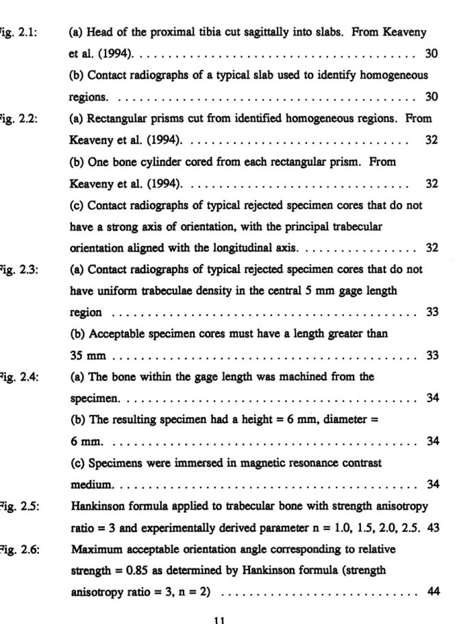
Fig. 2.1: (a) Head of the proximal tibia cut sagittally into slabs. From Keaveny et al. (1994) ... 30 (b) Contact radiographs of a typical slab used to identify homogeneous regions. ... 30 Fig. 2.2: (a) Rectangular prisms cut from identified homogeneous regions. From

Keaveny et al. (1994). ... 32 (b) One bone cylinder cored from each rectangular prism. From

Keaveny et al. (1994) ... 32 (c) Contact radiographs of typical rejected specimen cores that do not have a strong axis of orientation, with the principal trabecular

orientation aligned with the longitudinal axis ... 32 Fig. 2.3: (a) Contact radiographs of typical rejected specimen cores that do not

have uniform trabeculae density in the central 5 mm gage length

region ... 33 (b) Acceptable specimen cores must have a length greater than

35 mm ... .... ... 33 Fig. 2.4: (a) The bone within the gage length was machined from the

specim en... 34 (b) The resulting specimen had a height = 6 mm, diameter =

6 mm. ... 34 (c) Specimens were immersed in magnetic resonance contrast

medium ... 34 Fig. 2.5: Hankinson formula applied to trabecular bone with strength anisotropy

ratio = 3 and experimentally derived parameter n = 1.0, 1.5, 2.0, 2.5. 43

Fig. 2.6: Maximum acceptable orientation angle corresponding to relative strength = 0.85 as determined by Hankinson formula (strength

(12)

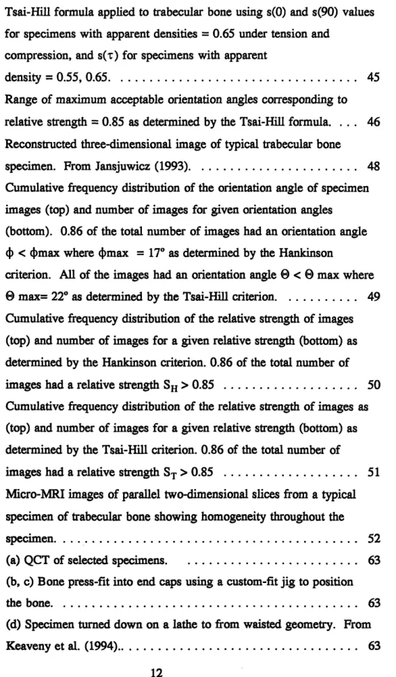
Fig. 2.7: Tsai-Hill formula applied to trabecular bone using s(0) and s(90) values for specimens with apparent densities = 0.65 under tension and

compression, and s(r) for specimens with apparent

density = 0.55, 0.65 . ... 45 Fig. 2.8: Range of maximum acceptable orientation angles corresponding to

relative strength = 0.85 as determined by the Tsai-Hill formula ... 46 Fig. 2.9: Reconstructed three-dimensional image of typical trabecular bone

specimen. From Jansjuwicz (1993). ... 48 Fig. 2.10: Cumulative frequency distribution of the orientation angle of specimen

images (top) and number of images for given orientation angles (bottom). 0.86 of the total number of images had an orientation angle 4) < 4max where 4)max = 170 as determined by the Hankinson

criterion. All of the images had an orientation angle O < 8 max where 8 max= 22* as determined by the Tsai-Hill criterion. ... 49 Fig. 2.11: Cumulative frequency distribution of the relative strength of images

(top) and number of images for a given relative strength (bottom) as determined by the Hankinson criterion. 0.86 of the total number of images had a relative strength SH > 0.85 ... 50 Fig. 2.12: Cumulative frequency distribution of the relative strength of images as

(top) and number of images for a given relative strength (bottom) as determined by the Tsai-Hill criterion. 0.86 of the total number of

images had a relative strength ST > 0.85 ... 51 Fig. 2.13: Micro-MRI images of parallel two-dimensional slices from a typical

specimen of trabecular bone showing homogeneity throughout the specim en... 52 Fig. 3.1: (a) QCT of selected specimens . ... 63

(b, c) Bone press-fit into end caps using a custom-fit jig to position the bone. ... 63 (d) Specimen turned down on a lathe to from waisted geometry. From Keaveny et al. (1994)... 63

(13)

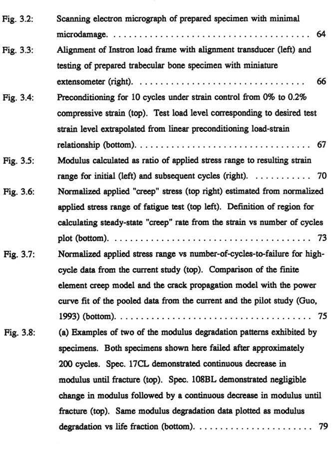
Fig. 3.2: Scanning electron micrograph of prepared specimen with minimal

microdam age. ... 64 Fig. 3.3: Alignment of Instron load frame with alignment transducer (left) and

testing of prepared trabecular bone specimen with miniature

extensometer (right). ... 66 Fig. 3.4: Preconditioning for 10 cycles under strain control from 0% to 0.2%

compressive strain (top). Test load level corresponding to desired test strain level extrapolated from linear preconditioning load-strain

relationship (bottom)... 67 Fig. 3.5: Modulus calculated as ratio of applied stress range to resulting strain

range for initial (left) and subsequent cycles (right). ... 70 Fig. 3.6: Normalized applied "creep" stress (top right) estimated from normalized

applied stress range of fatigue test (top left). Definition of region for calculating steady-state "creep" rate from the strain vs number of cycles plot (bottom). ... 73 Fig. 3.7: Normalized applied stress range vs number-of-cycles-to-failure for

high-cycle data from the current study (top). Comparison of the finite element creep model and the crack propagation model with the power curve fit of the pooled data from the current and the pilot study (Guo, 1993) (bottom)... 75 Fig. 3.8: (a) Examples of two of the modulus degradation patterns exhibited by

specimens. Both specimens shown here failed after approximately 200 cycles. Spec. 17CL demonstrated continuous decrease in modulus until fracture (top). Spec. 108BL demonstrated negligible change in modulus followed by a continuous decrease in modulus until fracture (top). Same modulus degradation data plotted as modulus degradation vs life fraction (bottom). ... 79

(14)

(b) Same modulus degradation patterns as in Fig. 3.8a, but the

specimens shown here failed after approximately 30,000 cycles. Spec. 44AL demonstrated continuous decrease in modulus until fracture (top). Spec. 27AL demonstrated negligible change in modulus followed by a continuous decrease in modulus until fracture (top). Same modulus degradation data plotted as modulus degradation vs life fraction

(bottom). ... 80 Fig. 3.9: (a) Stress-strain loops exhibited increasing non-linearity and hysteresis

and decreasing secant modulus. Both specimens (top and bottom) had similar fatigue lives (Nf = 200) but different minimum strain (%) at failure. ... 81

(b) Stress-strain loops exhibited increasing non-linearity and hysteresis and decreasing secant modulus. Both specimens (top and bottom) had similar fatigue lives (Nf = 20,000) but different minimum strain (%) at failure. ... 82 Fig. 3.10: (a, b) Examples of typical specimens that demonstrated the classical

rapid primary, slow secondary, and rapid tertiary regimes of creep (top and bottom)... 83 Fig. 3.11: Log-log plot of steady-state "creep" rate vs applied normalized stress

(top). Log-log plot of applied normalized stress vs time-to-failure (middle). Log-log plot of secondary-state "creep" rate vs time-to-failure (bottom). ... 84

(15)

List of Tables

Table 1.1 Summary of the determinants of fatigue properties of cortical bone ... 21 Table 2.1 Ultimate failure data for Tsai-Hill criterion ... 41 Table 3.1 Slopes and intercepts from fatigue experiments ... 76 Table 3.2 Comparison of slopes with low-cycles data ... 77

(16)

(17)

Chapter 1 Introduction: load.

..

unload.

.

.load.

.unload...

1.1 Role of fatigue in stress fractures, bone remodelling, and

spontaneous fractures

Normal activity such as breathing, walking, lifting objects, rising from a chair, and bending over exposes bone in vivo to repetitive, low-intensity loading. Although these cyclic loads produce stress levels lower than those required to fracture a bone specimen under static loading, they can result in damage at the microstructural level (Carter et al., 1981a; Carter and Hayes, 1977a; Schaffler et al., 1989). Not all loads necessarily result in damage to bone; however, microstructural damage in the form of microcracks, microfractures, or microcalli has been observed in individual trabeculae of the lumbar spine (Vernon-Roberts and Pirie, 1973), acetabulum (Ohtani and Azuma, 1984), femoral head (Benaissa et al., 1989; Dunstan et al., 1990; Freeman et al., 1974; McFarland and Frost, 1961; Todd et al., 1972; Urovitz et al., 1977; Wong et al., 1985), and proximal tibia (Pugh et al., 1973a) of post-mortem human specimens. Microstructural damage induced by repetitive loading has been hypothesized to play a significant role in stress fractures (Morris and Blickenstaff, 1967; Devas, 1975;

Griffiths et al., 1971), bone remodelling (Pugh et al., 1973b), spontaneous fractures in the elderly (Dunstan et al., 1990, Freeman et al., 1974; Urovitz et al., 1977; Wong et al., 1985), aseptic necrosis of the femoral head (McFarland and Frost, 1961),

degenerative joint disease (Radin et al., 1973b, Benaissa et al., 1989), and other bone disorders (Ohtani and Azuma, 1984).

1.1.1 Stress fractures

Fatigue damage accumulation can result from high levels of stress repeated over shorter periods of time and may be the major etiology of stress fractures

(18)

and shaft, tibia, fibula, and spine) in highly active patient populations (military

recruits, high performance athletes, and recreational athletes) (Morris and Blickenstaff, 1967; Devas, 1975; Griffiths et al., 1971). Cases of stress fractures generally have the following characteristics:

1) not associated with a single or traumatic event;

2) associated with activities involving repetitive loading of the involved bone; 3) preceded by symptoms of impending fracture (joint tenderness and swelling) without radiographic evidence of fracture;

4) symptoms subside while at rest for a period of time;

5) if radiographic signs are seen they are in the form of a fracture line or associated with callus formation;

6) if stress fractures occur they are in the form of blunt, brittle fracture planes (Nunamaker et al., 1990).

Stress fractures were first clinically reported in 1865 by army surgeons who observed painful, swollen feet in army recruits with no medical history of a specific trauma, after long periods of marching. When radiography was invented in 1895, the stress fractures were identified by doctors to occur in the metatarsals. Stress fractures often occur during prolonged exercise and are especially common in the metatarsals of military recruits, as well as runners (Meurman and Elfving, 1980; Matheson et al., 1985; Giladi et al., 1986; Krause and Thompson, 1944; Morris and Blickenstaff, 1967). Other clinical reports of stress fractures in athletes include ballet dancers and gymnasts who fracture the pars interarticularis (Pennel et al., 1985), and golfers who fracture the hook of the hamate (Daffner, 1978). A better understanding of stress fracture etiology could help develop training regimes and therapies that would more efficiently maintain soldiers and athletes at the boundary between maximum

performance and incipient fatigue failure. 1.1.2 Bone remodelling

Bone is a major and dynamic reservoir for calcium and phosphate with the processes of bone formation and resorption being tightly regulated. In the adult, bone

(19)

is constantly being remodelled to maintain an adequate supply of relatively low mineral density bone to subserve mineral homeostasis; this process involves up to 15% of the total bone mass per year (Ganong, 1981). Remodelling has also been proposed to function as a method of preventing the accumulation of fatigue damage. Although it is widely assumed that mechanical stresses influence the remodelling processes of bone (Wolff's law), neither the mathematical laws relating bone remodelling to the stress/strain environment nor the control systems which mediate these processes are understood. Proposed controlling mechanisms of bone remodelling have included micro fatigue damage, stress generated potentials, hydrostatic pressures on the extracellular fluids under load and alterations in cell membrane diffusions due to direct load (Goldstein et al., 1990). The remodelling response is therefore believed to be a reparative adaptive response to fatigue damage caused by daily repeated loading.

1.1.3 Age-related spontaneous fractures

During growth phases, formation exceeds resorption and the skeletal mass increases. Equal rates of formation and resorption prevail until ages 40 to 50 years, at which time resorption begins to exceed formation and the total bone mass slowly decreases (Ganong, 1981). The rate at which bone turns over may decrease with age

and this reduced rate of bone remodelling may compromise the ability to repair fatigue microcracks. If damage accumulates faster than it can be repaired, microcracks may

accumulate during years of repetitive loading, compromising bone strength, and

perhaps culminating in spontaneous fracture. Consequently, it is hypothesized that the fatigue behavior of bone may be a factor in the etiology of spontaneous fractures.

Approximately 10% of the 250,000 hip fractures and 50% of the 500,000 age related spine fractures that occur each year in the United States are believed to be

spontaneous fractures that result not from any obvious trauma, but rather from cyclic loading of normal activity (Freeman et al., 1974). Women are especially affected because they have a smaller bone mass and a more rapid rate of senescent loss than men (Ganong, 1981) with more than 40% of women 70 years of age or older experiencing one or more fractures (Christiansen, 1991). In addition to the loss of

(20)

function and associated risk of morbidity to the individual, the estimated annual medical cost for spontaneous hip and spine fractures may be over $1 billion (Keaveny and Hayes, 1993). As the elderly population increases with improved health care, the number of fractures and associated costs are expected to increase exponentially.

Thus, understanding the fatigue behavior of bone is essential from three perspectives: as the major etiologic factor in stress fractures, as a possible stimulus for bone remodelling, and as a possible etiologic factor in age-related spontaneous

fractures. Additionally, since most of the components of the skeletal system are subjected to repetitive loads during normal daily activity, the fatigue properties of bone are important simply to understand the normal behavior of bone (Choi and Goldstein, 1992).

1.2 Investigating bone fatigue properties and mechanisms

The fatigue properties of bone can be investigated by using either

contemporary concepts of fracture mechanics, or traditional concepts of stress and strain and applying them to cyclic loading conditions. In both approaches, the objective is to describe the strength of bone for a given number of load cycles and determining the material properties independent of the geometry. This chapter will focus on investigations using the latter approach to study the fatigue properties of the two types of bone--cortical and trabecular bone.

Cortical bone represents 80% of the total by mass and is typified by the thick shafts of the appendicular skeleton (arms and legs). Trabecular bone constitutes 20% and makes up most of the axial skeleton (vertebrae, skull, ribs) and bridges the center of the long bones (Ganong, 1981). In contrast to cortical bone, few controlled

experiments have been performed on trabecular bone primarily because the

heterogeneity of trabecular bone results in large data scatter, confounding the precision of analyses (Keaveny and Hayes, 1993).

(21)

1.2.1 Determining fatigue properties experimentally

In experiments where traditional engineering techniques are used to study fatigue behavior, standard specimens of bone are tested at a fixed level of stress or

strain and cyclically loaded to fracture. Tests are performed at different stress levels and the fatigue life corresponding to each stress level is found. Fatigue fracture characteristically occurs at stress levels that are substantially lower than the monotonic strength.

1.2.2 Fatigue properties of cortical bone

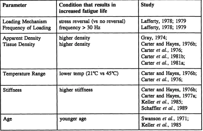
Ever since traditional engineering techniques were first used to determine the fatigue life of compact bone specimens (Evans and Lebow, 1957), the fatigue behavior of cortical bone has been studied extensively. The parameters which have been investigated as determinants of the fatigue properties of cortical bone are loading mechanism, frequency of loading, apparent density, tissue density, temperature range, anatomic location and microstructure, stiffness, and age (Table 1.1).

(22)

Table 1.1 Summary of the determinants of fatigue properties of cortical bone

Parameter Condition that results in Study

increased fatigue life

Loading Mechanism stress reversal (vs no reversal) Lafferty, 1978; 1979 Frequency of Loading frequency > 30 Hz Lafferty, 1978; 1979

Apparent Density higher density Gray, 1974;

Tissue Density higher density Carter and Hayes, 1976b;

Carter et al., 1976; Carter et al., 1981b; Carter et al., 1981a; Temperature Range lower temp (21°C vs 45°C) Carter and Hayes, 1976b;

Carter et al., 1976;

Stiffness higher stiffness Carter and Hayes, 1976b;

Carter and Hayes, 1977a;

Keller et al., 1985;

Schaffler et al., 1989

Age younger age Swanson et al., 1971;

Keller et al., 1985

The fatigue behavior of cortical bone is much like that of composite materials. In composite materials, microscopic cracks appear as the result of repetitive loading (Jamison et al., 1984). These cracks tend to run along lamellar interfaces, extending fatigue life by diverting energy from the propagation of transverse cracks which would cause more immediate failure (Kelly and Davies, 1965). In bone, similar cracks are normally present, and are differentiated from artifactual cracks by en bloc staining with basic fuchsin (Burr et al., 1985; Mori and Burr, 1993). The number of such cracks increases following repetitive loading (Burr et al., 1985; Mori and Burr, 1993). As damage accumulates through cyclic loading, there is a progressive loss of stiffness and strength (Carter and Hayes, 1977a; Carter and Hayes, 1977b; Keller et al., 1985; Schaffler et al., 1989; Pattin and Carter, 1990). Distinctly different types of bone microdamage are created by tensile and compressive loading. Fatigue damage created by tensile loading is characterized by separation at cement lines and interlameller

(23)

cement bands, and also by microcracking in the interstitial bone. Fatigue by

compressive loading results in oblique cracking and longitudinal splitting (Carter and Hayes, 1971; Carter and Hayes, 1977b).

1.2.3 Fatigue properties of trabecular bone

The fatigue characteristics of trabecular bone are virtually unknown. Recently, fatigue experiments on individual trabeculae and cortical bone have suggested that trabecular bone tissue has a lower fatigue strength and lower moduli than cortical bone tissue (Choi and Goldstein, 1989; Ashman and Rho, 1988; Choi et al., 1989, 1991; Ku et al., 1987; Kuhn et al., 1989; Mente and Lewis, 1989; Townsend and Rose, 1975). The difference in moduli and fatigue resistance was hypothesized to be the result of the different microstructure, mineralization, and collagen fiber orientation in the two tissues (Choi and Goldstein, 1989; Martin, 1991). Cortical bone tissue is arranged in layers of lamellae with relatively uniform mineralization. Trabecular bone is formed by surface remodelling with a higher turnover rate than cortical bone (Parfitt, 1983), thereby producing more cement lines and variable orientation. This microstructure may result in more local stress concentrators in the trabecular bone, explaining its lower fatigue resistance when compared to cortical bone.

1.2.4 Fatigue mechanisms of cortical bone

Since fatigue behavior is such an important aspect of the material properties of bone, much interest has developed in the actual mechanism of fatigue damage

accumulation; however, the fatigue mechanisms are complex and still not fully understood.

A series of both experimental and theoretical studies (Carter and Caler, 1983, 1985; Caler and Carter, 1989) addressed the fatigue behavior of cortical bone. Their first study investigated the possibility that in stress-controlled cyclic tensile loading, the failure of bone is a time-dependent phenomenon in which creep-fracture may play a significant role. Stress-controlled fatigue tests in fully reversed tension-compression and in cyclic tension loading, and tensile creep-fracture tests at constant stress levels were conducted. A time-dependent failure model with a tensile loading history predicted quite well the time to failure for the cyclic tension fatigue specimens,

(24)

suggesting that creep damage plays an important role in cyclic tension fatigue specimens.

Further exploring the contribution of creep damage in fatigue loading, Carter and Caler (1985) expanded their cumulative damage model for bone fracture to account for combined creep damage and fatigue damage. The damage model predicted bone fracture from a summation of only two independent processes--creep and fatigue, where the creep-fatigue interaction was assumed to be zero. The creep and fatigue damage fractions were calculated using empirical constants derived from their previously conducted creep-fracture and fatigue-fracture experiments (Carter and

Caler, 1983). The model attempted to describe the fracture behavior of bone under various loading histories and was successful in describing the influence of loading rate

on monotonic tensile strength, the time to failure in constant stress creep-fracture tests, and bone fracture in zero-tension and tension-compression cyclic loading. Caler and Carter then investigated applications of the cumulative damage model previously presented and observed the nature of material damage created under various loading histories (1989). This study was the first attempt at defining some fundamental features of bone damage in cyclic and creep loading. Fatigue tests were conducted in tension, compression, and reversed loading with a tensile mean stress. Bone displayed poor creep-fracture properties in both tension and compression. The fracture surfaces of the tensile creep specimens were distinctly different than those of the compressive specimens. The study suggested that in cortical bone, creep damage dominates in the low-cycle failure regime, while fatigue damage dominates in the high-cycle

regime.

1.2.5 Fatigue mechanisms of trabecular bone

Although data on the fatigue behavior of trabecular bone data are more limited than that available for cortical bone, a recent study of bovine trabecular bone

demonstrated fatigue behavior similar to that of cortical bone (Michel et al., 1993). Modulus degradation as a function of the number of cycles was distinctively different for high-cycle and low-cycle fatigue, suggesting differences in the response of

(25)

and creep damage accumulation for an idealized trabecular bone specimen were developed, and the predicted number-of-cycles-to-failure were compared with the experimental data (Guo et al., 1994). Predictions by the slow crack propagation model agreed well with the experimental data for the low-stress, high-cycle range, and

predictions by the creep analysis model agreed well with the experimental data for the high stress, low-cycle range. These results are consistent with previous findings on cortical bone and with the hypothesis that trabecular bone fails by creep in the low-cycle fatigue regime and by microcrack damage accumulation in the high-low-cycle fatigue regime.

1.2.6 Improved testing methods

The data describing the fatigue behavior of trabecular bone and its comparison with that of cortical bone should be carefully interpreted, however. Researchers in the late 1980's addressed the accuracy of the experimental methods used to measure the mechanical properties of trabecular bone and identified artifacts associated with load frame compliance, and frictional and damage end effects (Linde and Hvid, 1987; Linde and Hvid, 1989; Linde et al., 1992; Odgaard et al., 1989; Odgaard and Linde,

1991). These experimental artifacts arise with traditional platen-to-platen compression tests in which the modulus is derived from the relative displacements between the platens. As a result, the modulus can be over- or under-estimated. To improve accuracy in mechanical testing of trabecular bone, the Orthopaedic Biomechanics Lab has developed a test protocol involving reduced-section cylindrical specimens with brass endcaps in which strain is measured directly by a miniature extensometer. This technique has been demonstrated to minimize experimental artifacts (Keaveny et al.,

1994). With the exception of some pilot data, the relation between fatigue loading and the number-of-cycles-to-failure has not been characterized previously using this test protocol.

An inherent assumption of the improved test protocol is that trabecular bone specimens are homogeneous in density and have a longitudinal axis which is aligned with the principal trabecular orientation. The compressive strength and stiffness of trabecular bone have been shown to be sensitive to both anisotropy (Brown and

(26)

Ferguson, 1980; Ciarelli et al., 1991; Townsend, 1975) and density (Carter, 1976, 1977; Ciarelli et al., 1991; Ducheynes, 1977). Thus unintentional off-axis testing can potentially introduce scatter in the experimental data and confound the interpretation of uniaxial mechanical test data. To decrease such scatter, as part of the standard

technique to select specimens, contact radiographs of each cylindrical specimen are reviewed to select specimens of homogeneous density whose longitudinal axis is aligned with the principal trabecular orientation. The spatial variation of trabecular architecture within specimens harvested using this technique has not yet been quantified.

1.3 Objectives

* To validate the use of contact radiography in selecting trabecular bone

specimens of homogeneous density whose longitudinal axis is aligned with the principal trabecular orientation.

* To accurately characterize the compressive fatigue behavior of devitalized bovine trabecular bone by additional mechanical testing of reduced-cylindrical specimens under loads corresponding to low stress levels normalized by the initial modulus.

1.4 Organization

The following chapter (Chapter 2) describes the use of micro-magnetic resonance imaging to validate a standard technique for selecting trabecular bone

specimens. This technique is then used to select specimens for mechanical testing in Chapter 3. Chapter 3 describes these fatigue tests and presents data acquired in this study, pooled with previously reported pilot data (Guo, 1993). The pooled

experimental data are then compared with predictions of two-dimensional finite

element models for creep and slow crack growth in idealized trabecular bone as a first step in identifying the fatigue damage mechanism involved. The final chapter

(Chapter 4) summarizes the work and includes recommendations concerning areas for further research.

(27)

Chapter 2 Using Micro-Magnetic Resonance Imaging (pMRI) to

Validate a Standard Technique for Selecting

Trabecular Bone Specimens

2.1 Introduction

The compressive strength and stiffness of trabecular bone have been shown to be sensitive to both anisotropy (Brown and Ferguson, 1980; Ciarelli et al., 1991; Townsend, 1975) and density (Carter and Hayes, 1976, 1977; Ciarelli et al., 1991; Ducheyne, 1977). A wide range of material anisotropy exists in trabecular bone, with specimens typically being either orthotropic or transversely isotropic with an isotropic plane perpendicular to the axis of symmetry. Thus, unintentional off-axis fatigue testing could introduce substantial scatter in the experimental data and cause

significantly more error in some specimens than in others. Such errors due to off-axis measurements reduce the predictive power of the resulting power regression between stress (or strain) and fatigue life. An inherent assumption in uniaxial compressive fatigue tests (Chapter 3) of trabecular bone is that the axis of loading for each specimen is aligned with the principal trabecular orientation.

Initial studies of the properties of trabecular bone loaded specimens along the anatomic axes (anterior-posterior, medial-lateral, or inferior-superior) (Kuhn et al., 1989; Ciarelli et al., 1991) or anatomic directions (i.e. along femoral neck) (Lotz, 1990). Variability in trabecular bone moduli of as much as 100-fold have been observed from one location to another within the same metaphysis of the human proximal femur (Goldstein et al, 1983). Material properties of trabecular bone vary tremendously among different skeletal sites primarily because the degree of anisotropy and apparent density varies with anatomical position.

(28)

More recently, regions of homogeneous density in which the material axes are aligned with the specimen axes have been identified using contact radiography of slabs of trabecular bone from which parallelepipeds are cut. The success of this technique in aligning the material and specimen axes was investigated using surface optical stereology to measure the angle between the principal material and specimen axes (Borchers, 1991). Although optical stereology is an excellent method for quantifying the external morphology of trabecular bone, it is inadequate to characterize the internal trabecular architecture.

Previous investigators have noted the potential for wide variation in trabecular bone orientation throughout small specimens of bone. Variability in percent

orientation of as much as 30% has been observed in an 8 mm cube of human trabecular bone (Goulet et al., 1988). Thus, two-dimensional morphologic analysis may not be sufficiently accurate enough to identify specimens which are misaligned with the loading axis due to intra-specimen variations in architecture.

Three-dimensional reconstruction of the architecture of trabecular bone specimens can now be achieved with micro-magnetic resonance imaging (pMRI). Micro-magnetic resonance imaging protocols have been fully developed (Hipp and Jansjuwicz, 1993; Jansjuwicz, 1993) to produce visual reconstructions of bone specimens at a resolution comparable to what can be obtained with micro-computed tomography (Kuhn, 1990) and serial sectioning (Odgaard et al., 1990). Algorithms using image processing routines such as thresholding functions and fourier transforms, and bone morphology routines such as the method of directed secants have also been developed and validated (Hipp and Jansjuwicz, 1993; Jansjuwicz, 1993) to calculate mean intercept lengths, anisotropy, volume fraction, and the principal orientations together with the three-dimensional reconstructions.

Currently, as part of the standard technique for selecting specimens (described below) a set of contact radiographs of each cylindrical specimen is reviewed to select specimens of homogeneous density whose longitudinal axis is aligned with the

principal trabecular orientation. The spatial variation of trabecular architecture within specimens harvested using this technique has not yet been quantified. Because

(29)

off-axis testing confounds the interpretation of uniaxial mechanical test data, the longitudinal specimen axis must be aligned with the principal trabecular orientation during fatigue tests. Thus the aim of this study was to validate the use of contact radiography in selecting trabecular bone specimens of homogeneous density whose longitudinal axis is aligned with the principal trabecular orientation. To characterize the principal material axes over the entire volume, three-dimensional micro-magnetic resonance images were obtained. Using methods based on directed secants, alignment of the longitudinal axis with the principal trabecular orientation and degree of anisotropy were determined. Additionally, area fraction of solid in serial slices through a typical specimen was determined to investigate the homogeneity of

density.

2.2 Materials and methods

2.2.1 Standard technique for selecting specimens for mechanical testing

Cylindrical cores of bovine trabecular bone were harvested from fresh proximal tibia following the Orthopaedic Biomechanics Laboratory's standard procedure for preparation of bovine trabecular bone specimens (Figs. 2.1- 2.3). After the fresh bone was procured from a local slaughterhouse (Bertolino Beef Co., South Boston, MA, USA), the soft tissue and fascia were removed from the tibia, and the head of the proximal tibia was separated from the diaphysis using a band saw (1 HP #C.92 H, Food Machinery of America, Buffalo, NY, USA). The proximal head was then cut sagittally into 12 mm thick slabs (Fig. 2.1a). Contact radiographs (Kodak X-OMAT TL Diagnostic Film #158 3293, Eastman Kodak, Rochester, NY, USA) of these slabs

were taken (Faxitron Model #43855A A04, Hewlett-Packard, McMinnville, OR, USA)

and used to identify regions of trabecular bone of homogeneous density and anisotropy (Fig. 2.1b). From these identified homogeneous regions, 40 mm x 12 mm x 12 mm rectangular prisms were traced using a template and then cut with the band saw, ensuring that the principal orientation of the trabeculae within the central 5 mm gage length was aligned with the prism axes (Fig. 2.2a). Using a diamond-tipped coring

(30)

(a)

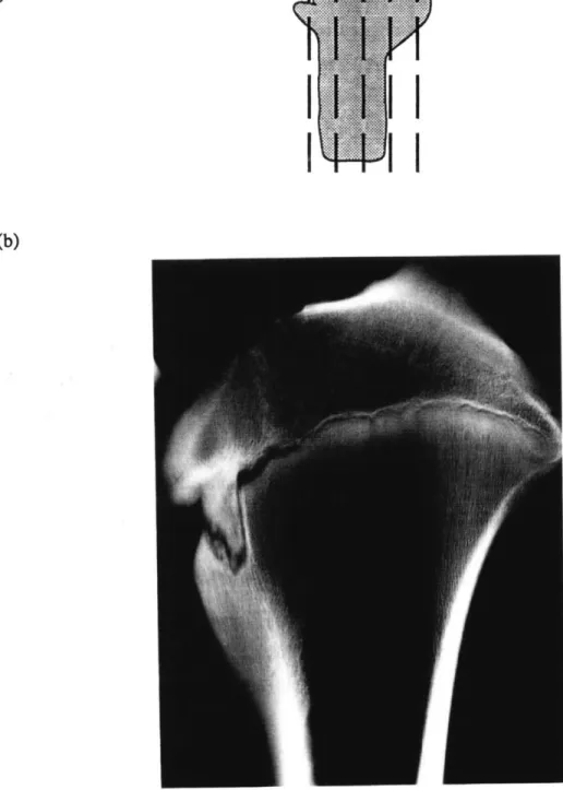
(b)

Figure 2.1: (a) Head of the proximal tibia cut sagittally into slabs. From Keaveny et al. (1994).

(b) Contact radiograph of a typical slab used to identify

(31)

tool (Starlite, Rosemont, PA, USA) one bone cylinder (diameter, d = 8.3 mm) was cored from each of these prisms (Fig. 2.2b).

Contact radiographs of the cylinders were independently reviewed by three investigators with regard to three criteria: orientation, density, and length. Acceptable specimen cores were required to have 1) a strong axis of orientation, with the principal orientation of the trabeculae being aligned longitudinally with the core axis (Fig. 2.2c); 2) uniform trabeculae density in the central 5 mm gage length region where failure would occur (Fig. 2.3a); 3) a length greater than 35 mm to accommodate the brass end caps (to be added in the next stage), the central 5 mm waisted gage length region, and 3 -4 mm of bone between the waisted length and the end caps (Fig. 2.3b). Only specimens meeting all three requirements advanced to the final stages of specimen preparation for mechanical testing (Fig. 2.3c).

2.2.2 Specimen Preparation for Micro-Magnetic Resonance Imaging (pMRI) Because the specimen selection and preparation method is rather labor-intensive, this study was coordinated with an unrelated study so that a single set of specimens was used in both studies. One of the objectives of the other study was to quantify modulus errors in the traditional compression test (Keaveny et al., 1995). In that study, specimens were loaded in compression for ten cycles under strain control at +/- 0.4% and then for ten cycles under displacement control at 0.06 mm. These

applied loads are well below the threshold for altering any of the structural properties of trabecular bone, permitting the use of these specimens in this study.

After mechanical testing, the bone within the gage length was machined from the specimen with a low speed saw (Isomet, Buehler Corp., Lake Bluff, IL, USA) equipped with a diamond wafering blade operating under copious irrigation (Fig. 2.4a). The resulting specimen had a 1:1 aspect ratio with height and diameter measuring 6 mm (Fig. 2.4b). The specimens were prepared for micro-magnetic resonance imaging following standard lab procedure (OBL SOP #IA_M_1, Version #2) (Hipp and

Jansjuwicz, 1993; Jansjuwicz, 1993). The marrow space contents were removed from the bone specimens by ultrasonic agitation (Fisher Ultrasonic Cleaning System, Fisher Scientific, Pittsburgh, PA, USA) with a 1:3 bleach:water solution. After 15 - 20

(32)

(a)

~f:

(c)

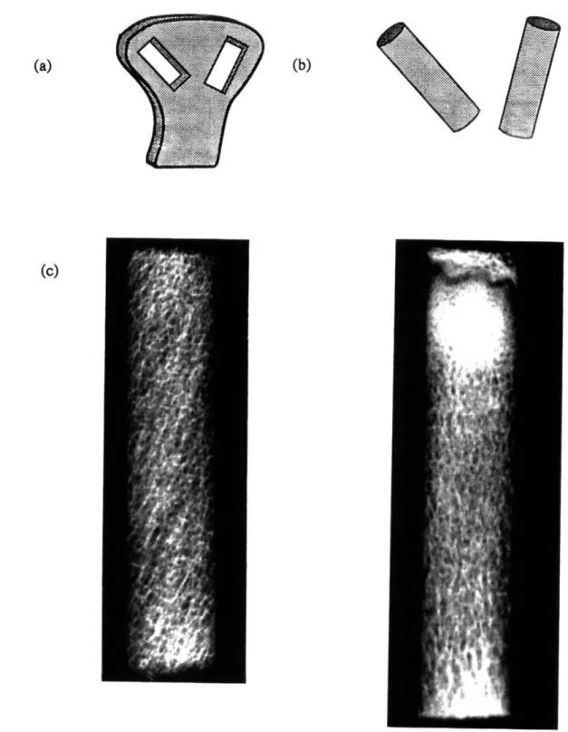
Figure 2.2: (a) Rectangular prisms cut from identified homogeneous regions. From Keaveny et al. (1994). (b) One bone cylinder cored from each

rectangular prism. From Keaveny et al. (1994). (c) Contact radiographs of typical rejected specimen cores whose longitudinal axis is not aligned with the principal trabecular orientation (left) or do not have a strong axis of orientation (right).

(b)

(33)

(a)

>35

mm

6 mm

Endcap/bone interface

3 to 4 mm

5 mm

3 to 4 mm

Endcap/bone interface

S

-

8.3 mm

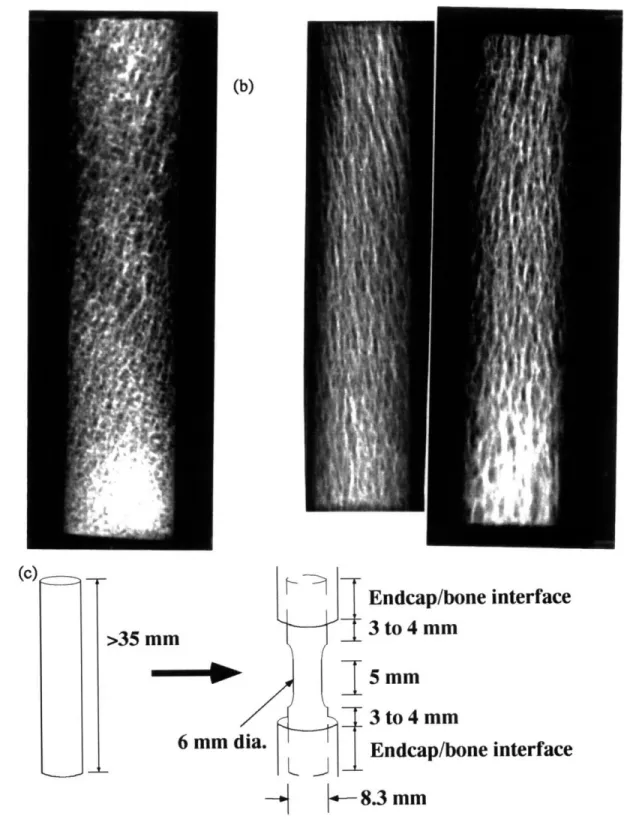
Figure 2.3: (a) Contact radiograph of a typical rejected specimen core that does not have uniform trabeculae density in the central 5 mm gage length region.

(b) Examples of acceptable specimen cores (c) Acceptable cores must have a length greater than 35 mm.

(C)

L

(34)

CMR

tube

Specimen excised

from gauge length

1:1 aspect ratio

specimen

Specimen immersed

in 0.2% Gadolinium

solution

Figure 2.4: Specimen preparation for micro-magnetic resonance imaging following standard lab procedure. (a) The bone within the gage length was machined from the specimen. (b) The resulting specimen had a height = 6 mm, diameter = 6mm. (c) Specimens were immersed in magnetic resonance

contrast medium.

6 mm

_{6 mm}

dia.

(35)

minutes of agitation, the cloudy solution was replaced with fresh bleach solution. Ultrasound was continued and the process repeated until the dilute bleach solution remained clear but for no longer than a total of 45 minutes.

The specimens were then placed in magnetic resonance compatible tubes and immersed in magnetic resonance contrast medium of 0.2 mg/ml solution of

gadopentetate dimegumine per 100 ml of distilled water (Fig. 2.4c). Replacing the marrow phase with the gadopentetate solution provided a more homogeneous imaging medium. The immersed specimens were degassed under vacuum to remove any trapped air bubbles that would otherwise appear as areas of low signal intensity in the image and would be incorrectly identified as bone. Specimens remained under

vacuum until the bubbling rate of the specimens was negligible. 2.2.3 Micro-Magnetic Resonance Imaging

The degassed, immersed specimens were imaged following standard lab procedure (OBL SOP #IA_M_1,Version #2) (Hipp and Jansjuwicz, 1993; Jansjuwicz,

1993) using a Bruker AM spectrometer (Bruker Instruments, Inc., Billerica, MA) with micro-imaging accessory and a 10 mm HI radio frequency coil. The field of view was set to 7.841 mm in all directions and the raw data stored to a 128 x 128 x 128 array. The resolution obtained using these parameters was 61.3 microns along each edge of

the voxels. An algorithm with low and high thresholds was used to classify each voxel in the variance image as being either bone or marrow space (Hipp and

Jansjuwicz, 1993; Jansjuwicz, 1993). The binary three-dimensional image files were viewed using Sunvision (SUN Microsystems, Mountain View, CA, USA) and

AVS-based custom software (Application Visual System (AVS), Advanced Visual Systems Inc., Waltham, MA, USA).

2.2.4 Analysis of Micro-Magnetic Resonance Images

Material symmetry and orientation angle Each reconstructed three-dimensional image was automatically centered and a 5000 micron (5.0 mm) diameter spherical region of interest was chosen. Methods based on directed secants were used to

analyze this constant volume of bone (Snyder, 1991; Hipp and Jansjuwicz, 1993; Jansjuwicz, 1993). The three-dimensional mean intercept length (MIL) vector was

(36)

determined for each of 128 randomly oriented rotations of a three-dimensional

collinear test line array at a parallel testline spacing of 200 microns. The MIL vector was a statistical estimate of the average length between phase boundaries within one phase and was defined as:

MIL = 1 total length of test lines * bone vol fraction (2.1)

1 * no. of intersections between test lines and phase boundaries

An ellipsoid was fit to the MIL vectors and the properties of the ellipsoid were used to describe anisotropic properties of the bone sample The angle between the longitudinal axis of the specimen and the principal trabecular orientation was determined by

solving the equation and orientation of the ellipsoid with respect to the principal axes and was defined as the angle between the projection of the MIL vector on the x-y plane and the maximum principal MIL vector. The degree of material anisotropy in one principal direction i was defined as:

prin value in dir. i - mean prin value of all 3 dir.

degree of anisotropy =

_{mean principal value}

(2.2)

where the principal values were the lengths of the individual ellipsoid semi-axis lengths. The mean trabecular thickness was also determined for each image; it was given by:

2 * bone vol. fraction

mean trabecular thickness = (2.3)

boundary interface length betwn bone & marrow

Homogeneity. The variability in homogeneity through a specimen was investigated in a typical specimen. Using the post-processing software (Application Visual System (AVS), Advanced Visual Systems Inc., Waltham, MA, USA), the reconstructed image could be sectioned in any plane to visualize the internal structure of the specimen. Five serial slices parallel to the longitudinal axis of the specimen were imaged using a high resolution monochrome videocamera (CCD 72 Series Camera, Dage-MTI, Inc., Michigan City, IN, USA) equipped with a 50 mm lens

(37)

(Olympus Corp., Japan) and a video digitizing system (SUN Videopix board, SUN Microsystems, Mountain View, CA, USA). Each digitized image was 640 by 480 pixels, resulting in a resolution of 20 microns per pixel. An algorithm based on iterative edge detection was used to automatically determine a grey-level threshold delineating bone and marrow spaces (Snyder et al., 1990; Hipp and Jansjuwicz, 1993; Jansjuwicz, 1993). The two-dimensional mean intercept length vectors of a circular

test region were determined for each of 64 evenly spaced rotations of a dimensional collinear test line array at a testline spacing of 200 microns. The two-dimensional MIL vector was also defined by Eqn. (2.1), with bone area fraction substitute for the bone volume fraction. An ellipse was fit to the MIL vectors and the orientation of the major principal material axis was estimated from the ellipse fit to these data. The area fraction of the solid was determined through a pixel counting routine within the circular test region:

area fraction = number of pixels representing bone (2.4)

area fraction = (2.4)

total number of pixels

2.2.5 Criteria for determining acceptable range of specimen alignment

A Hankinson-type relationship and Tsai-Hill formula were used to determine an acceptable degree of misalignment of the angle between the longitudinal axis of the specimen and the principal trabecular orientation that still ensures accuracy in the strength measurements.

Hankinson formula. The original Hankinson relationship was formulated for determining the compressive strength of wood (Hankinson, 1921) and has been

adapted to successfully predict the off-axis strength of human cortical bone (Reilly and Burstein, 1975), but not yet applied to trabecular bone. The Hankinson-type formula relates the off-axis ultimate compressive strength of a trabecular bone specimen to the

(38)

s() - s(90) s(0)

s(O) =

(2.5)

s(90) cos"( ) + s(O) sin"(0)

where ( = angle between the longitudinal axis of the specimen and the principal trabecular orientation (orientation angle)

s(() = off-axis ultimate compressive strength at angle D

s(O) = ultimate longitudinal compressive strength i.e. strength of a trabecular bone specimen in which the longitudinal axis of the specimen is perfectly aligned with the principal trabecular

orientation (( = 0")

s(90) = ultimate transverse compressive strength i.e. strength of a trabecular bone specimen in which the longitudinal axis of the specimen is perpendicular to the principal trabecular orientation ((D = 90*)

n = experimentally derived parameter

The ultimate compressive strength of a specimen as determined by the Hankinson formula (Eqn. 2.5) can be expressed as a fraction of the ultimate longitudinal

compressive strength; we define relative strength SH as determined by the Hankinson formula:

off-axis ultimate strength _ s( (26)

relative strength = S ultimate longitudinal compressive strength -s(O)

The relative strength SH as determined by the Hankinson-type relationship is

dependent upon the strength anisotropy ratio and an empirically determined constant n. We define strength anisotropy ratio R as:

strength anisotopy ratio= R = ultimate longitudinal compressive strength _ s(0) (2.7)

(39)

The strength anisotropy ratio for the ultimate compressive strength of trabecular bone specimens is 2.9 (Pinilla et al., 1993); here, we take a value of 3. The constant, n, has not been empirically determined for trabecular bone. We assumed a value of n =

2.0 for trabecular bone as determined for wood (Forest Products Laboratory, 1990) and cortical bone when tested in compression (Reilly and Burstein, 1975). Using a

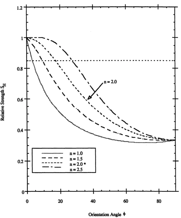
strength anisotropy ratio of 3 and assuming n = 2.0 in the Hankinson-type relationship (Eqn. 2.6), the relative strength of a trabecular bone specimen SH was plotted against orientation angle (D.

(40)

Tsai-Hill formula. The Tsai-Hill formula predicts failure strengths in off-axis uniaxial tensile tests and is based on the von Mises failure criterion which was

originally applied to homogeneous and isotropic bodies (Hull, 1981). The criterion was later expanded and modified to anisotropic bodies and applied to successfully predict the variation of strength with angle for composite materials such as carbon

fiber-epoxy resin laminae. The Tsai-Hill formula accounts for the interactions between the tensile stresses which lead to transverse tensile cracks and the shear stresses which lead to intralaminar cracks on the same fracture plane. The criterion can be used to predict the failure strength in off-axis tests on unidirectional laminae and may be expressed as:

cos'I 1 1 sin' 2 (2.8)4

s(8) =[cs4+( - 1)si cssinecose + (2.8)

s(0)2 s()-2 (0 )2 s(90)2

where E = angle between the longitudinal axis of the specimen and the principal trabecular orientation (orientation angle)

s(O) = off-axis ultimate strength at angle E

s(O) = ultimate longitudinal strength i.e. strength of a

trabecular bone specimen in which the longitudinal axis of the specimen is perfectly aligned with the principal trabecular

orientation (0 = 0°)

s(90) = ultimate transverse strength i.e. strength of a

trabecular bone specimen in which the longitudinal axis of the specimen is perpendicular to the principal trabecular orientation (0 = 90*)

(41)

The ultimate strength of a specimen as determined by the Tsai-Hill criterion (Eqn. 2.8) can be expressed as a fraction of the ultimate longitudinal strength; we define relative strength ST as determined by the Tsai-Hill criterion:

off-axis ultimate strength s(O)

relative strength = ST ultimate longitudinal strength s(O)

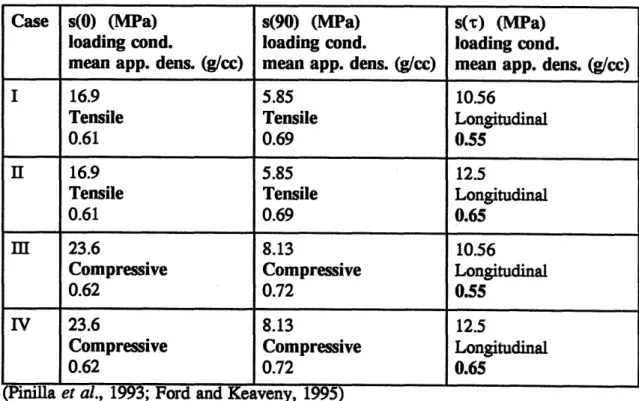
Recently available longitudinal and transverse ultimate tensile and compressive strength and shear strength data for bovine trabecular bone specimens (Pinilla et al., 1993; Ford and Keaveny, 1995) were used to plot the relative strength ST of a specimen against orientation angle 0 for four different cases of loading and mean apparent density. Ultimate tensile and compressive failure data for specimens with mean apparent densities of approximately 0.65 g/cc, and ultimate shear data for specimens with mean apparent densities of 0.55 g/cc and 0.65 g/cc were plotted. Table 2.1: Ultimate failure data for Tsai-Hill criterion

Case s(0) (MPa) s(90) (MPa) s(r) (MPa)

loading cond. loading cond. loading cond.

mean app. dens. (g/cc) mean app. dens. (g/cc) mean app. dens. (g/cc)

I 16.9 5.85 10.56

Tensile Tensile Longitudinal

0.61 0.69 0.55

II 16.9 5.85 12.5

Tensile Tensile Longitudinal

0.61 0.69 0.65

iI 23.6 8.13 10.56

Compressive Compressive Longitudinal

0.62 0.72 0.55

IV 23.6 8.13 12.5

Compressive Compressive Longitudinal

0.62 0.72 0.65

(42)

Acceptable degree of misalignment using Hankinson and Tsai-Hill. For a specimen in which the longitudinal axis of the specimen is perfectly aligned with the principal trabecular orientation, the relative strength is 1.0. Specimens having a compressive strength greater or equal to 0.85 of the longitudinal ultimate compressive

strength s(0) were considered to have acceptable alignment. From the plot of the Hankinson formula applied to trabecular bone, the maximum acceptable degree of misalignment of the angle between the longitudinal axis of the specimen and the principal trabecular orientation Imax corresponding to s(I)/s(0) = 0.85 was

determined. Similarly, from the plot of the Tsai-Hill formula applied to trabecular bone, the maximum acceptable degree of misalignment of the angle between the longitudinal axis of the specimen and the principal trabecular orientation 0.m corresponding to s(O)/s(0) = 0.85 was determined.

2.3 Results

2.3.1 Maximum acceptable degree of misalignment

Hankinson formula. Using a strength anisotropy ratio of 3 and assuming n = 2 for trabecular bone in the Hankinson-type relationship (Eqn. 2.6), the relative strength SH of a trabecular bone specimen was plotted against orientation angle (Fig. 2.5).

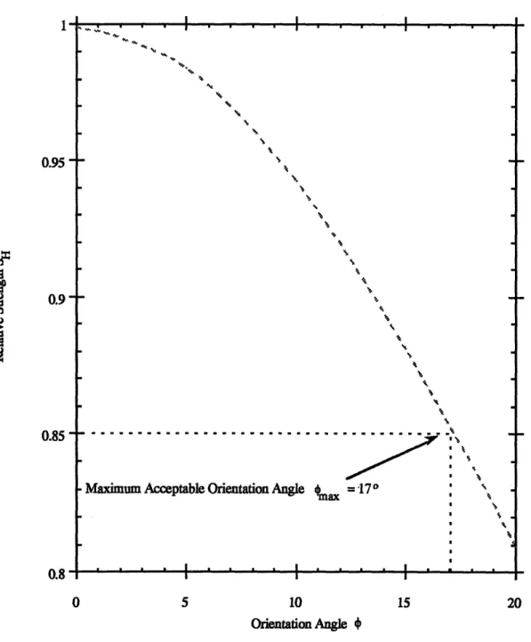
From Fig. 2.6, we found (max = ±17*, where (ma is the maximum acceptable degree

of misalignment of the angle between the longitudinal axis of the specimen and the principal trabecular orientation corresponding to SH = s()/)s(0) = 0.85.

Tsai-Hill formula. Using available ultimate failure strength data (Table 2.1) in the Tsai-Hill criterion (Eqns. 2.8 and 2.9), the relative strength ST of a trabecular bone specimen was plotted against orientation angle for four cases (Fig. 2.7). From Fig. 2.8, we found 220 < IOmax < 330, where O0m is the maximum acceptable degree of

misalignment of the angle between the longitudinal axis of the specimen and the principal trabecular orientation corresponding to ST = s(0)/s(0) = 0.85. The lower bound of the range of acceptable orientation angles (Omax = 22*) resulted from Case HI test conditions (Table 2.1). Case III used s(@) for specimens with a mean apparent

(43)

0.1 0.4 0., 0." 0 20 40 60 80 Orientation Angle 4

Figure 2.5: Hankinson formula applied to trabecular bone with strength anisotropy ratio = 3 and experimentally derived parameter n= 1.0, 1.5, 2.0, 2.5.

(44)

I I

-_{Maximum Acceptable Orientation Angle max}

...

=170

- .

-Orientation Angle €

Figure 2.6: Maximum acceptable orientation angle corresponding to

relative strength = 0.85 as determined by Hankinson

formula (strength anisotropy ratio = 3, n = 2).

-0.95

0.95-0.9 ~i~ 0.85- 0.8-· 1 I _ _ I I I · _ I I __ _ __ _ _ _ _ I - I - | . . . . |

(45)

0.i 0.1 0.: 0.! 0 20 40 60 80 Orientation Angle 6

Figure 2.7: Tsai-Hill formula applied to trabecular bone using s(0) and s(90) values for specimens with apparent densities = 0.65 g/cc under tension and compression, and s(z) for specimens with apparent densities = 0.55, 0.65 g/cc.

(46)

1.05 0.95

0.5

0.85 0.1 0 5 10 15 20 25 30 35 40 Orientation Angle 0

Figure 2.8: Range of maximum acceptable orientation angles corresponding

to relative strength = 0.85 as determined by the Tsai-Hill formula.

(47)

density = 0.55 g/cc, and s(0) and s(90) of specimens loaded in compression. The

upper bound of the range of acceptable orientation angles (ma x = 330) resulted from

Case II test conditions (Table 2.1). Case II used the s(r) of specimens with a mean apparent density = 0.65 g/cc, and s(0) and s(90) of specimens loaded in tension. 2.3.2 Material symmetry and orientation angle

One three-dimensional micro magnetic resonance image was obtained for each of twelve bovine trabecular bone specimens. Images were repeated for two of the specimens, resulting in 14 total images (Fig. 2.9). The orientation angle ranged from 2.130 - 20.630 (Fig. 2.10), with the relative strength SH as determined by the

Hankinson formula ranging from 0.81 - 1.0 (Fig. 2.11) and the relative strength ST as determined by the Tsai-Hill criterion ranging from 0.87 - 1.0 (Fig. 2.12). Twelve of the 14 images had an acceptable degree of misalignment as determined by the

Hankinson formula (orientation angle (D < 170), and all 14 of the images had an

acceptable degree of misalignment as determined by the Tsai-Hill formula (orientation angle 0 < 220). Four of the fourteen images were classified as transversely isotropic and ten as orthotropic. The mean trabecular thickness ranged from 0.26 -0.52 mm.

2.3.3 Homogeneity

The variation in homogeneity through the depth of a specimen was investigated for a typical specimen (Fig. 2.13). Analysis of five serial slices parallel to the

longitudinal axis for the specimen estimated the mean area fraction of the solid was 0.36 (SD 0.035), the mean ratio of major to minor mean intercept lengths was 1.31

(SD 0.14), and the mean orientation of the major principal material axis was 3.2* (SD 3.80).

2.4 Discussion

Although previous investigators have observed a wide variation in orientation over small regions of trabecular bone, our micro-magnetic resonance imaging results indicate that our current selection technique using contact radiographs ensures an

(48)

Figure 2.9: Reconstructed three-dimensional image of typical trabecular bone specimen. From Jansjuwicz (1993).

Compressive high cycle at low strain fatigue behavior of bovine trabecular bone

ABSTRACT

Acknowledgements

Table of Contents

59

59

61

61

62

68

69

74

List of Figures

List of Tables

Chapter 1

Introduction: load.

..

unload.

.

.load.

.unload...

1.1 Role of fatigue in stress fractures, bone remodelling, and

spontaneous fractures

1.2 Investigating bone fatigue properties and mechanisms

1.3 Objectives

1.4 Organization

Chapter 2

Using Micro-Magnetic Resonance Imaging (pMRI) to

Validate a Standard Technique for Selecting

Trabecular Bone Specimens

2.1 Introduction

2.2 Materials and methods

were taken (Faxitron Model #43855A A04, Hewlett-Packard, McMinnville, OR, USA)

(a)

(b)

(a)

(b)

(a)

>35

mm

6 mm

Endcap/bone interface

3 to 4 mm

5

mm

3 to 4 mm

Endcap/bone interface

S

8.3 mm

CMR

tube

Specimen excised

from gauge length

1:1 aspect ratio

specimen

Specimen immersed

in 0.2% Gadolinium

solution

6 mm

dia.

degree of anisotropy =

(2.2)

s(O) =

(2.5)

2.3 Results

...

0.5

2.3.3 Homogeneity

2.4 Discussion