Comparison study of SEASAT scatterometer and conventional wind fields

COMPARISON STUDY OF SEASAT SCATTEROMETER AND CONVENTIONAL WIND FIELDS

by

Kristine Holderied B.S'., Oceanography United States Naval Academy

1984

SUBMITTED IN PARTIAL FULFILLMENT OF THE REQUIREMENTS FOR THE DEGREE OF

MASTER OF SCIENCE at the

MASSACHUSETTS INSTITUTE OF TECHNOLOGY and the

WOODS HOLE OCEANOGRAPHIC INSTITUTION September, 1988

This thesis is not subject to U.S. copyright.

Signature of the author - I. - - - -

-Joint Program in Oceanography,

Massachusetts Institute of Technology -Woods Hole Oceanographic Institution

/ I / A Certified by Carl Wunsch Thesisp pervisor " V ___1IP_*____~_Yn~__l___I_1Yllqllll~_ LI Accepted by Carl Wunsch

Chairman, Joint Committee for Physical Massachusetts Institute of Technology -Woods Hole Oceanographic Institution.

ADO~~ ;~~4 ~

COMPARISON STUDY OF SEASAT SCATTEROMETER AND CONVENTIONAL WIND FIELDS

by

Kristine Holderied

Submitted to the Massachusetts Institute of Technology-Woods Hole Oceanographic Institution Joint Program

in September, 1988 in partial fulfillment of the requirements for the Degree of Master of Science

ABSTRACT

A demonstrated need exists for better wind field information over the open ocean, especially as a forcing function for ocean circulation models. Microwave scatterometry, as a means of remotely sensing surface wind information, developed in response to this requirement for a surface wind field with global coverage and improved spatial and temporal resolution. This development led to the 1978 deployment of the SEASAT Satellite Scatterometer (SASS). Evaluations of the three months of SEASAT data have established the consistency of SASS winds with high quality surface wind data from field experiments over limited areas and time periods. The directional ambiguity of the original SASS vectors has been removed by Atlas et al. (1987) for the entire data set, and the resulting SASS winds provide a unique set of scatterometer wind information for a global comparison with winds from conventional sources.

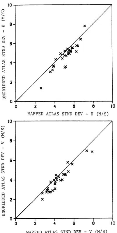
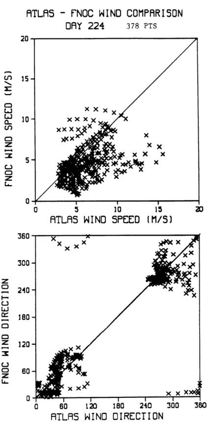
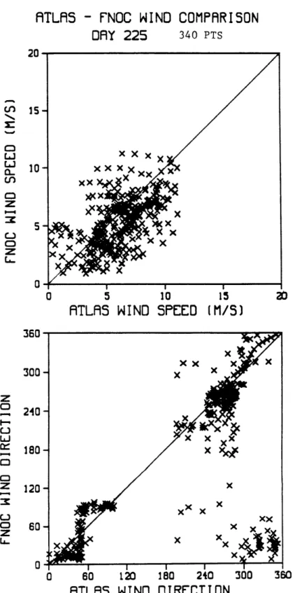
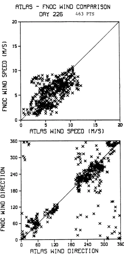
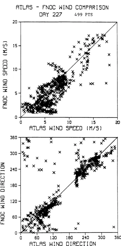
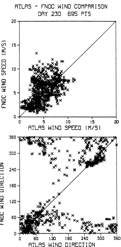
A one-month (12 August to 9 September 1978) subset of these dealiased winds, in the western North Atlantic, is compared here with a conventional, pressure-derived wind field from the 6-hourly surface wind analyses of the Fleet Numerical Oceano-graphic Center (FNOC), Monterey, CA. Through an objective mapping procedure, the irregularly spaced SASS winds are regridded to a latitude-longitude grid, facilitating statistical comparisons with the regularly spaced FNOC wind vectors and wind stress curl calculations. The study includes qualitative comparisons to synoptic weather maps, calculations of field statistics and boxed mean differences; scatter plots of wind speed, direction, and standard deviation; statistical descriptions of the SASS-FNOC difference field, and wind stress curl calculations.

The SASS and FNOC fields are consistent with each other in a broad statistical sense, with wide scatter of individual values about a pattern of general agreement. The FNOC wind variances are slightly smaller than the SASS values, reflecting smoothing on larger spatial scales than the SASS winds, and the SASS mean values tend to be slightly higher than the FNOC means, though the increase is frequently lost in the large scatter. Exceptions to the pattern of relatively small consistent variations between the two fields are the pronounced differences associated with extremely strong winds, especially during Hurricane Ella, which traveled up the East Coast of the United States during the latter part of the study period. These large differences are attributed mainly to differences in the inferred positions of the pressure centers and in the response at the highest wind speeds (> 20m/s). The large statistical differences between the SASS and FNOC fields, present under high wind conditions, may yield significantly different ocean forcing, especially when the strong winds persist over longer periods of time. Under less intense wind conditions, usually prevailing over the ocean, the two fields correspond well statistically and the ocean responses forced by each should be similar.

Thesis supervisor: Dr. Carl Wunsch

Cecil and Ida Green Professor of Physical Oceanography Secretary of the Navy Research Professor

Table of contents A bstract . . . . Chapter 1: Introduction. ...

Chapter 2: Background . . . . ... .

Wind velocity and wind stress . . . . . .

Ocean wave spectrum and radar backscatter. Empirical U-to-a relation . ...

Chapter 3: SEASAT Scatterometer (SASS). SASS geophysical algorithm ...

SASS performance evaluations. . . . . .

SASS data reprocessing. ...

Chapter 4: Data description and handling ...

Objective mapping procedure . . . .

Chapter 5: Results and discussion. . . . .

Field statistics . . . . .

Ungridded Atlas winds . . . . .

Mapped Atlas winds . . . . .

FNOC winds. ...

Boxed mean differences . . . . .

Scatter plots of wind speed and direction. Difference field statistics . . . .

Wind stress curl . . . . . Chapter 6: Summary and conclusions ...

. . . .10 . . . . .12 . . . . .16 . . . .18 S . . . . .21 . . . .23 S . . . . .26 . . . .28 S . . . . .30 S . . . . .32 39 42 42 43 45 47 49 53 57 . . . .60

Appendix 1. Aspects of atmospheric boundary layer theory. Appendix 2. Ocean waves and energy transfer . . . . . . Appendix 3. Aspects of radar scatter theory . . . . . References . . . . Tables . . . . Figures _{. . . .} S . . . . .65 S . . . . .71 S . . . . .73 . . . .77 . . . .82 . . . . 152 Acknowledgments _{. . . . .217}

1. Introduction

The large-scale oceanic circulation has been extensively studied, especially over the past 100 years, and considerable advances have been made in theoretical under-standing of the processes involved. A critical part of this study is the attempt to understand the forcing that drives the circulation. The two major driving forces are the stress due to wind blowing over the ocean surface and the buoyancy-driven mo-tions due to thermohaline processes. The directly wind-driven circulation is confined to, and dominates, flow in the upper layers of the ocean. It is primarily horizon-tal motion, but convergence and divergence of this flow give rise to vertical motion, creating regions of upwelling or downwelling. Theoretical study of the wind-driven circulation was motivated initially by attempts to account for observed surface cur-rents, starting with the work of Nansen (1898), Ekman (1905), and Sverdrup (1947). Further progress was associated with attempts to explain westward intensification, reflected in strong western boundary currents (Stommel, 1948; Munk, 1950). This work established our basic understanding of how wind stress drives the ocean circu-lation, and subsequent developments are reviewed by Veronis (1981) and Pond and Pickard (1983).

While wind-forcing is accepted as the primary driving force in the upper layers, themohaline forces also play a significant role in ocean circulation, especially in the lower layers where they tend to dominate. In this case, water movements are associ-ated with changes in density, either from temperature or salinity changes. In the ocean these changes normally occur as an increase in density at the surface, either directly through cooling or indirectly through freezing and subsequent production of more saline water. Such processes cause a buoyancy-driven vertical flow that is followed by horizontal flow due to continuity requirements or to geostrophic currents resulting from the changes in density. Thermohaline processes are frequently associated with changes in weather and climate, and may also be strongly influenced by the wind field, especially in terms of surface heat fluxes and downward mixing in the surface layer. Therefore, the wind field plays a most critical role, both directly and indirectly,

in forcing the ocean circulation, and its specification is crucial to reaching a more complete understanding of that circulation through theory and model developments.

However, the development and verification of these theories and their applica-tion to global circulaapplica-tion models are hampered by the current lack of good wind fields over the open ocean. The most frequently used fields for wind-forcing are av-eraged estimates of the wind stress, available both globally (Hellerman, 1967,1968; Han and Lee, 1983; Hellerman and Rosenstein, 1983) and for particular regions (for example: Bunker, 1976; Hastenrath and Lamb, 1977; O'Brien and Goldenberg, 1982). These climatological values are averaged across monthly, seasonal, and annual peri-ods, generally from all available ship reports in the chosen period, extending over a considerable length of time and employing some wind speed to stress conversion. In the case of the Hellerman and Rosenstein (1983) analyses, for example, ship reports from 1870 to 1976 were used to form monthly averages, and stress was computed from wind speed based on a wind speed and atmospheric stability dependent drag coefficient. Many uncertainties still exist in the details of the wind speed to wind stress relationship (discussed in Section 2), and these parameterization issues limit the accuracy of the stress fields. However, a greater limitation is posed by the long averaging periods, which result in a considerable loss of information on the temporal variability of the wind field. In addition to the wind stress fields derived from long-term ship reports, daily maps of wind speed derived from surface pressure analyses, supplemented by ship and buoy reports, are available. While these are available much more frequently than the averaged stress fields, they are not direct measurements of the surface wind field, but inferred from the much smoother quantity of pressure. Spatial resolution is considerably reduced due to these inherently large pressure field scales, and small, intense circulations may be lost in the broader scale unless they are observed independently.

The insufficient amount of wind measurements, sparse global coverage, and re-stricted scales of conventional wind information available limit the studies that can be done. In particular, conventional sources generally provide winds only at larger scales (> 1000 km), geostrophically from surface pressure fields, and at very small

scales (< 10 km), from ship and buoy reports. There is virtually no resolution of the intermediate spatial scales, which contain significant energy and are important to atmospheric forcing of the ocean (Freilich and Chelton, 1986). The conventional data also lack sufficient temporal resolution for modeling the temporal variability of the upper ocean, especially over larger areas. The absence of information at shorter time and space scales forces reliance on long time-averaged data for modeling purposes. These averages are of some use in studying the mean circulation, but lose much of the variability needed to drive the more complex models. Some studies of the temporal and spatial variability in realistic wind fields, as well as of the impact of that variation on ocean motions, have been conducted, though the studies are necessarily limited

by the coarse resolution of climatological wind fields (for example: Willebrand, 1978;

Willebrand et al., 1980; Muller and Frankignoul, 1981). The forcing effect of wind stress on the ocean surface is a major determinant for ocean waves and upper ocean currents. Knowledge of these motions is crucial to many fields, including basic oceano-graphic research, climate studies, and practical ocean operations. The interrelation of these motions and the wind forcing can be more fully evaluated only if an accu-rate, global wind field is available for input into the numerical models. Conventional sources of wind field information, including many different types of observations and analyses, do not currently provide sufficient information for this purpose, and a re-peated, global measurement of wind stress (or velocity) over the ocean would therefore be a unique contribution (O'Brien, 1982).

The microwave scatterometer, yielding wind velocity as inferred from surface roughness measured by reflected radiation, was developed to provide this missing in-formation. Mounted on aircraft or, more effectively, on satellites, this instrument has the potential to provide a more accurate, variable, global wind field at higher temporal and spatial resolutions than currently available. The SEASAT Satellite Scatterometer (SASS), launched in 1978, was the first operational scatterometer system to be flown. The three months of data returned from that mission is a unique set of information that has yet to be repeated, since no scatterometer has flown since. Details of basic scatterometer theory, the SEASAT mission, and SASS itself are given in Section 2.

1_~V--The wind forcing information derived from scatterometer measurements provides both new research opportunities with the expanded information it makes available, as well as very useful information for immediate use in practical operations. Improved

specification of the wind forcing would allow ocean modelers to better estimate ocean behavior, and therefore reach a more thorough understanding of upper ocean physics. The scatterometer can resolve winds on the intermediate spatial scales and the global, shorter time scales that are missing in conventional data. This information would con-tribute greatly to modeling of the temporal and spatial variability of the upper ocean (Freilich and Chelton, 1986). The ocean is forced by the wind stress, both directly, and indirectly through mass field adjustments, and the stress field must be incorporated into any realistic ocean model. Current parameterizations of thermodynamic forcing, including the surface fluxes of sensible and latent heat, use aerodynamic bulk for-mula models that incorporate wind velocity. So, better wind field information would improve our understanding and modeling capability of both wind stress and ther-modynamic forcing. In the absence of good forcing fields from conventional sources, oceanographers are restricted to artificial forcing fields, at best adjusting the sparse information currently available to obtain reasonable results from the model. Some of the new ocean modeling opportunities opened up by the more accurate, extensive wind fields provided by the scatterometer include: 1) improved ocean basin models, 2) improved wind forcing related process studies, 3) improved prediction and moni-toring of ocean climate phenomena such as El Nifio, and 4) better input for practical, daily ocean forecasting models.

Scatterometer derived wind fields will also have valuable applications to meteo-rological research and weather prediction, and to a better understanding of processes at the air-sea interface. Assimilation of scatterometer data may have a significant impact on numerical weather prediction, through both model initialization and sub-sequent updates (Cane et al, 1981; Yu and McPherson, 1979; 1981; Duffy and At-las, 1986; Harlan and O'Brien, 1986). The additional information provided by the scatterometer is particularly important in data sparse areas, such as the Southern Ocean. Scatterometer derived wind fields also have important applications to naval

and commercial ocean operations. These include tactical weather forecasting, acous-tic conditions forecasting, surf forecasting for amphibious operations, ship routing, and warnings of potentially catastophic situations. More commercial uses include oil platform design, drilling schedules, and commercial fishing schedules. The potential cost savings associated with these scatterometer wind applications are summarized in O'Brien (1982).

Better vector wind stress fields will be needed to drive the increasingly sophis-ticated ocean models, designed to resolve temporal and spatial variability on finer scales. The choice of a particular wind field for this forcing is crucial when we want to more accurately establish the influence of the "real" surface winds on ocean cir-culation. At that point it becomes crucial to pick the "best" wind field available, in terms of accurately reproducing the actual winds with sufficient resolution at the desired scales. Even if it is not possible to determine which is best in an absolute sense, it is important to at least reach a good understanding of the differences be-tween the various wind fields available, especially in their ultimate impact on model output. In particular, when conventional and scatterometer derived fields are consid-ered as alternative forcing functions, the presence or absence of significant differences between the two can influence the decision to deploy a scatterometer in the first place. If no significant differences are found between the two fields, over the time and space scales of interest, then the effort and expense necessary to develop and maintain an operational scatterometer is not justified, since it would not significantly augment information already available. This study does not intend to address the more comprehensive question of the need for a scatterometer, assuming, as discussed briefly above, that this requirement is already well-established (Brown, 1983;1986; O'Brien, 1982). Rather, assuming that the scatterometer wind fields will be avail-able and will therefore compete with conventional winds as model input, this work seeks to examine the differences between these fields in a more detailed fashion. This is accomplished by qualitatively and quantitatively comparing two such fields, the conventional surface wind analyses from the Fleet Numerical Oceanographic Center (FNOC) in Monterey CA, and SEASAT Scatterometer winds from R. Atlas at the

Goddard Space Flight Center (GSFC) (Atlas et al., 1987), obtained through the Jet Propulsion Laboratory (JPL), Pasadena, CA. An overview of satellite scatterometry is provided in Section 2 to introduce some basic atmospheric boundary layer and mi-crowave backscatter concepts. Section 3 describes the SEASAT mission and SASS, and Section 4 provides a general description of the various data used and outlines the objective mapping procedure used to regrid the scatterometer winds. Section 5 pro-vides more detailed wind field statistics and various quantitative comparisons between

the scatterometer and conventional winds, including boxed mean differences, scatter plots of various quantities, difference field statistics, and wind stress curl calculations. Section 6 contains the summary and conclusions.

2. Background

The development of microwave scatterometer theory is based on studies of the atmospheric boundary layer, radar scatter, and ocean surface motions. Some of the basic concepts from these areas that apply directly to scatterometer work are reviewed here. The complex nature of the air-sea boundary makes quantifying and measuring physical processes there a difficult problem. Wind stress, r, represents the transfer of momentum from the atmosphere to the ocean. This transfer of momentum slows the air near the ocean surface, creating an atmospheric boundary layer. The vertical profile of wind velocity in the atmosphere is dominated by molecular processes in the few millimeters closest to the sea surface, with turbulent motions, governed by friction and buoyancy, dominating the rest of the surface layer (Stewart, 1985). At higher levels the surface effect diminishes and the geostrophic general circulation of the atmosphere governs the flow. The region most critical to scatterometer work is the 20 meters closest to the surface, and concentration on this region affects assumptions made about the relative dominance of various processes. In general, the wind velocity profiles are derived analytically, combining a logarithmic layer with an Ekman spiral modified by secondary flow for winds greater than 5 m/s (Brown, 1986). The various parameters and details behind this theory are discussed in more detail below and in

Appendix 1.

The study of atmospheric and surface boundary layers is based on formulas and empirical correlations that were originally derived from empirical studies. Many field experiments have been conducted to investigate the relevant processes, and then to adjust the formulas and refine the empirical constants (see Stewart, 1985 for partial review). Three quantities, the fluxes across the sea surface of horizontal momentum, sensible heat, and latent heat, are of particular interest in the 1 cm to 10 m surface layer where the surface effect dominates. Within this turbulent atmospheric surface layer, the fluxes are approximately constant with height and the wind and temperature profiles are logarithmic - with adjustments for stability (Halbertstam, 1980). Much study has been devoted to deriving the fluxes from wind speed and temperature

profiles. The similarity concepts of Obukhov (1946) and initial experiments of Monin and Obukhov (1954) are incorporated in most of the profile formulas. The vertical profile of wind velocity, and its relation to surface drag, or stress, strongly influences the transfer of energy from atmosphere to ocean. Wind stress, r, is accepted as the major driving force for large-scale ocean circulation. However, practical considerations have dictated that, rather than being measured directly, the wind stress is normally derived from wind velocity, U, usually measured at some distance above the ocean surface. This is a highly complicated relationship, dependent on the complex dynamics of the boundary layer at the air-ocean interface.

The scatterometer uses a measure of the surface roughness, determined from the reflection of microwave radiation, as an inferred measure of the air-sea energy transfer. The surface roughness can be connected to a particular geophysical parameter, such as wind velocity or wind stress, as well as to the backscattered power that forms the scatterometer signal. In practice, a direct relation is sought between the backscat-ter and a geophysical paramebackscat-ter, commonly chosen to be the wind velocity at some height above the surface. However, this relation has no direct physical basis, and is determined empirically. The theoretical justification for the empirical relation comes rather from our understanding of various parts of the process, and the interconnec-tion of quantities such as the wind velocity, wind stress, ocean wave spectrum, and backscattered radiation. The review of these basic concepts below is divided into three broad areas, the U-to-r relation, the impact of wind stress on the ocean wave spectrum, and the relation between the ocean wave spectrum and reflected radiation. These are examined in turn, followed by a discussion of their practical, but indirect application in the direct relation between wind velocity and reflected radiation. In a sense this discussion can be seen as describing two paths to the same goal, the first a multi-step, theoretical process and the second a single, empirical step, where the latter path is dependent on the principles established by the former.

Wind velocity and wind stress

The U-to-r relation is determined by converting the wind at some reference height, Urei, through the boundary layer, to a surface stress, r. This connection between the wind velocity profile and wind stress are of primary importance to scat-terometry. The interfacial momentum flux, or wind stress, can be defined as the average turbulent transfer of horizontal momentum from atmosphere to ocean by vertical air movements (O'Brien, 1982). For a constant wind, the wind stress is cal-culated from correlations between perturbations of the vertical and horizontal wind components, expressed as :

7 = pUW

where:

r = _{wind stress (N/m} 2₎

p = air density (kg/m3)

u,w = horizontal and vertical velocity (m/s) (Stewart, 1985)

The averaging period must be long enough to form stable averages of the turbulent properties, yet short enough for mean conditions to be steady. Times of 40 minutes to 1 hour are usually chosen. Compounding the complex theoretical issues in this relation are the practical difficulties inherent in measuring the relevant quantities. The ocean surface is a difficult environment to work in, and the critical turbulent time and space scales are relatively short. To circumvent the constraints of direct measurement, a series of empirical relationships (bulk or aerodynamic formulae) have been developed. These relate the wind stress to the wind velocity at some height, with the usual form:

r = _{pCDU ef}

where:

CD = drag coefficient

The exact formulation of the drag coefficient is still subject to considerable debate, and varies with wind speed and atmospheric stability, as discussed in Appendix 1. A commonly accepted formulation is that of Large and Pond (1981), which combines a constant value for CD at lower wind speeds (< 11 m/s) with an expression that is linearly dependent on wind speed at higher speeds (see Appendix 1 for the exact form).

The wind velocity profile near the surface varies sharply with height and depends on both r and atmospheric stability. The transfer of heat and momentum depend on turbulence generated by both wind shear and buoyancy (affected by temperature and humidity stratification). Shear dominates near the surface and buoyancy becomes relatively more important at some height above the surface. The influence of stability is illustrated by considering the case of cold air blowing over warmer water. Air is heated from below and rises, causing instability in the air column and enhancing the turbulence due to just the mechanical shear of the wind stress. In the opposite case, when warm air blows over cold water, there is a suppression of turbulence as cooling from below stably stratifies the air column. The impact of wind stress and stability on motions in the turbulent layer is described quantitatively by Monin-Obukhov similarity theory, discussed in more detail in Appendix 1. A primary result from these theories is that, assuming that the influence of atmospheric stability is weak, the wind velocity profile is logarithmic with height for neutral stability, and simply shifted by stability corrections. Under unstable conditions, or for a strongly stratified atmosphere, these formulations are no longer valid, but the condition of weak stratification is generally satisfied over widespread areas, except in the tropics where strong convection cells are common.

Though considerable debate still exists on some details of the theory and on the exact formulation of the relation, there is a generally accepted understanding of the wind stress-to-velocity connection. The choice of wind velocity in particular, and if so, at what height, as the relevant parameter to relate to microwave backscatter is a still greatly debated issue. The neutral stability wind at 19.5 m was chosen for the original processing of SEASAT scatterometer data, based on anemometer heights

aboard some weather ships. From boundary layer considerations, a better choice would be the wind velocity closer to the surface (such as at 10 m), or the friction velocity. Another alternative parameter, using the wind just above the surface, is discussed in a later section. Though the "best" parameter has yet to be decisively chosen, for the initial evaluations made for SASS development, the most practical choice was wind velocity. The boundary layer wind velocity theories described here provide justification for that particular choice, as they connect the wind velocity to wind stress. A factor requiring further evaluation is the effect of stratification, especially since it can have a significant influence at all scales. The parameterizations discussed here hold for relatively weak stratification effects, but are questionable under conditions where atmospheric stratification plays an important role, such as in the tropics. To isolate these effects for future uses, widespread measurements are needed of both the currently available sea surface temperature measurements, and the not yet generally available air temperature measurements over the ocean (Atlas et al., 1986). A more detailed parameterization of the effects of stability, along with better sea surface and air temperature observations would significantly improve and extend the range of scatterometer wind algorithms.

Wind stress and the ocean wave spectrum

Given some stress at the ocean surface, the next step is to determine how this transfer of momentum from the air is reflected in the ocean wave spectrum. Un-derstanding the processes behind this energy transfer is a fundamental problem of remote sensing. Important factors in the wind-wave relation include wave generation, wave-wave and wave-current interactions, wind strength, atmospheric stratification, sea surface temperature, and sea state. The ultimate goals are to determine how much energy is transferred from air to ocean, on what scales the transfer takes place, and how the energy is partitioned to various ocean features, in particular, waves and currents. Wind generated waves range from millimeters to hundreds of meters and, while there is considerable theoretical understanding of the longer gravity waves, the

~-_--LI- W

high-frequency end of the spectrum is much less well understood. Current theory holds that the short wavelengths reflect the surface response to the local wind field. As discussed in detail in the following section, scatterometers are designed to look at these wavelengths, in particular at the centimeter-length capillary waves. Some physical factors that influence the surface ripple field are: 1) the tangential and nor-mal stresses at the surface, 2) the fraction of momentum transfer going into capillary waves, 3) the magnitude and direction of the swell, 4) ocean currents and mixing, 5) wave history, 6) hydrostatic stability (Davidson et al., 1981). The lack of definitive descriptions of open ocean capillary waves and their relation to the surface fluxes has hindered theoretical understanding in this area. Evidence also exists that only a portion of the air-sea momentum transfer goes into these waves, and the assumption that the short waves reflect the entire momentum transfer, and therefore the wind stress, is not supported by any complete quantitative theory (Brown, 1986). Partial explanations are available for various processes, especially wave generation, growth, and interaction, but many critical effects have yet to be modeled, and a single, unified theory does not exist. Short waves are associated with skin friction-induced small-scale stress, and therefore do not account for the direct momentum transfer through form drag on long waves from pressure fluctuations (Brown, 1986). The partitioning of momentum transfer between shear stress and form drag is discussed in more de-tail in Appendix 2. Other unaccounted for factors that may distort the local wave field to local wind relationship include swell, usually generated at more distant loca-tions and unrelated to local winds, and momentum transfer to ocean currents, thus unavailable for wave generation. At present, the influence of uncorrelated swell and the momentum loss to currents are assumed to be small and are neglected. A short review of some theories and experiments on the basic physics behind the transfer of energy from air to water is given in Appendix 2. The concepts and studies discussed here provide the still rough theoretical understanding of the wind-wave relation used to justify scatterometer development. These present interpretations are supported by the generally good results gained from scatterometer measurements made thus far. Further refinements of the assumed stress-to-wave spectrum relation are still needed

to resolve effects such as the time response of wave formation, interference from other waves, and the effect of sea slicks.

Ocean wave spectrum and radar backscatter

The final step is to determine the ocean wave spectrum from information on surface roughness gained from reflected radiation, or backscatter. The interaction of electromagnetic radiation with the surface provides information on surface features, depending on the wavelengths of the radiation and the features. Extracting surface information from the power of the backscatter signal therefore requires knowledge of both scattering theory and surface characteristics. Details of relevant surface scat-tering principles are provided in Appendix 3. The primary radiation measure is the normalized radar cross section (NRCS), a' , a ratio of the reflected to incident energy across a unit surface area. The crucial problem is to characterize the shape of a0

for a given sea surface parameter, generally chosen to be the ocean wave spectrum. Scatter from the wavy ocean surface is described by two physical mechanisms, spec-ular and Bragg (or resonant) scatter, which depend on the incidence angle (angle between the radar beam and local surface vertical) and wavelength of the incident radiation, and on the wavelengths of the surface waves. Appendix 3 contains further descriptions of these scatter mechanisms, including the incidence angle dependence and ranges, and the adjustments needed to accomodate the multiple scales of oceanic motion. The most useful return for scatterometry is the resonant scatter from capil-lary waves, yielding both speed and direction information on the wave spectrum, and by association, on the surface stress or wind velocity.

These basic scattering concepts are complicated by the complex conditions actu-ally present on the sea surface. Wave tank and field experiments have shown spikes in backscatter returns due to sharp-crested waves that are close to breaking (Kwoh and Lake, 1984). The effect on a of rain striking the surface is significant, but not well understood. The capillary waves tend to be damped by rainfall, thus de-creasing backscatter return, but rain-generated ripples also appear, inde-creasing the

radar return. Some experimental evidence has shown ao to increase with rainfall (Moore et al., 1979), but more study is needed to determine the magnitude of this effect. Sea slicks can significantly affect backscatter as well (Huhnerfuss et al., 1983), and recent work further demonstrates the impact of wave slope and atmospheric strat-ification on the radar return (Keller et al., 1985). At higher wind speeds, when the surface is confused, with significant foam and spray coverage, the application of Bragg scatter theory is questionable and new models may be necessary (Atlas et al., 1986).

While microwave backscatter theory is reasonably well understood in terms of electromagnetic radiation principles, the precise connection to the short wave spectra is not well specified. Rather, as discussed in detail in Section 3, the assumed relation between the two is used to justify empirical models that relate backscatter to wind velocity and various parameters of the radar signal. Though these models produce realistic results and have been used with much success, they shed little light on the physical processes that link microwave backscatter and ocean wave spectra. Also, as discussed by Plant (1986), the current formulations of short wave spectra derived from physical principles (eg: Phillips, 1977; Kitaigorodskii, 1983; and Phillips, 1985) are not directly applicable to scatterometry, since they cannot account for the dramatic increase in the backscatter signal with the increase in wind speed (and therefore sur-face roughness). Addressing this question, Plant (1986) derives a form for the short wave spectrum that incorporates long wave-short wave interactions as well as wind input and dissipation. The expression for the short wave spectra is valid to second order in long wave slope, and is then used, for the case of locally generated seas, to develop an expression for ao , also valid to second order in long wave slope. This formulation allows a more detailed investigation of the effects of long wave slope and propagation on backscatter, through the tilting and hydrodynamic modulation of the short waves, but it is still a considerable simplification of actual ocean conditions. Assuming that the relevant parameter is the backscatter from capillary waves, in the real ocean these ripples (and therefore the associated aO signal) are modulated by ocean currents,internal waves, and sea state, and subject to tilt effects from longer

waves. Surface currents cause variations in a through their effects on waves, includ-ing changinclud-ing the direction of propagation and amplifyinclud-ing wave amplitudes by local velocity convergences. The effect of internal waves is not that pronounced at this scale, but sea state can have a significant impact (Atlas et al., 1986). The influence of sea state is especially important in rougher conditions, when foam, spray, and break-ing waves disrupt the surface and contaminate the backscatter return, often as signal spikes.

In the absence of detailed knowledge of the actual long wave field, the optimum conditions for scatterometry occur when equilibrium is reached by those waves approx-imately one order of magnitude longer than the capillary waves (Atlas et al., 1986). These conditions are assumed in scatterometer algorithm development, and though this steady state condition is typical for the open ocean, it will not hold near signifi-cant circulation features, such as fronts. In order to completely specify the modulation and tilt effects for future algorithms, more extensive and more highly resolved in situ ocean wave spectra information is needed. In addition to refining the empirical scat-terometer relations, this information could also provide a means of developing and validating theories on the physical processes discussed here. These scattering con-cepts, though simplifications of realistic conditions, are supported by the few exper-imental studies available (see Stewart, 1985 for summary). The difficulty of making simultaneous measurements of ocean wave spectra and backscatter has necessarily limited the amount of experimental evidence. While many questions still remain to be answered, there is increasing physical understanding of microwave backscatter, of the short ocean wave spectrum, and of the connection between them. Future study will be directed to quantifying the effects on microwave backscatter of rain, wave

slope, sea surface temperature, currents, internal waves, and breaking waves.

Empirical U-to-ao relation

The theories described above are used to establish a physical foundation, through a convoluted, multiple-relation process, on which to connect microwave backscatter

surface wind velocity. The response of short capillary waves to environmental changes at the air-sea interface, as measured by radar backscatter, is used to determine wind speed and direction. Given the theoretical support provided by these concepts, the practical application is to use that basis to justify seeking a direct relation between wind and the measured radar cross-section. The direct relation is established in three steps: 1) isolate the critical parameters, 2) establish the basic form of the equation (ie: power law, drag law, etc.), and 3) describe the detailed aspects of the model through empirical coefficients. Empirical studies have shown the dependence of ao on wind speed and wind direction relative to the horizontal antenna pointing angle as well as on the incidence angle, polarization, and frequency of the radar signal (Plant, 1986). Wind speed dependence is described by an adjusted power law while directional dependence is characterized by an approximately cos(2X) dependence on the relative azimuth angle, x. The empirical coefficients are derived by tuning the basic equation to a set of data, for which both the known and unknown variables have been found. An obvious limitation to this process is that tuning to a particular data set constrains the backscatter-to-wind relation to the range of conditions present in that data. The specific details of the a" -to-wind relation used for SEASAT scatterometer data are described in Section 3. It should be mentioned that the radar cross-section has been shown to correlate well with both wind velocity and friction velocity (Liu and Large, 1981). However, as mentioned above, due to the need for conventional measurements to validate the empirical relation, and to the relative unavailability of wind stress measurements, a wind velocity dependence was chosen for SEASAT. One problem with current formulations is an inconsistency between the parameterizations for neutral wind and friction velocity. The current choices of power law relations to backscatter for both are not compatible with the expected connection between the two for a neutrally stratified atmosphere (Pierson et al., 1986).

Recent theoretical and experimental evidence indicates that the capillary wave spectrum, and by assumption the microwave backscatter, correlates better with a

near-surface wind field characteristic, R, than with either the neutral wind or friction velocity (Pierson et al., 1986). This new parameter is expressed as:

R = ( 1) 1)2 C(A)

where:

U() = average wind at half a Bragg wavelength above the

surface

C(A) = phase speed of Bragg waves

A = Bragg wavelength

(Pierson et al.,1986)

This term is related to the normal stresses, and correlation with short wave spectra depends on the assumption that normal stresses dominate tangential stresses in wave generation (Atlas et al., 1986). Unlike a direct correlation of backscatter to friction velocity, use of R requires definition of the wind profile and specification of a drag coefficient, or friction velocity and roughness length (Pierson, et al., 1986). So the ap-plication of R with scatterometer data is similar to using the neutral stability winds, but with a characteristic that is more physically related to the surface roughness. These concepts may improve future scatterometer missions, but SEASAT data was processed with a o' -to-U relation and that will be emphasized here. Despite many unresolved issues, the available SASS results have demonstrated that useful correla-tions between microwave backscatter and a wind or surface roughness parameter can be found (Brown, 1986).

3. SEASAT Scatterometer (SASS)

A considerable microwave backscatter history culminated in the development

of the SEASAT scatterometer, commencing with experiments on radar sea clutter during and after World War II. The initial proposal to use microwave backscatter to determine winds at the ocean surface came from Moore and Pierson (1967). A history of the various initial experiments can be found in Moore and Fung (1979). Following the general procedures discussed above, various empirical forms were devel-oped for the backscatter-to-wind vector relation (Moore and Fung, 1979; Boggs, 1981; Jones et al., 1982; Schroeder et al., 1982a; Woiceshyn et al., 1986). The final choice for SEASAT, discussed in detail below, was a single power law relation with a least squares inversion (Moore and Fung, 1979; Jones et al., 1977). Following the SEASAT mission, the scatterometer model function was tuned through comparison with high quality surface wind data, primarily that collected in the Gulf of Alaska (GOASEX) and Joint Air-Sea Interaction (JASIN) experiments (Jones et al., 1982; Schroeder et al., 1982a, 1982b; Wurtele et al., 1982; Brown, 1983). Some results from these experiments are summarized following a more detailed description of the SEASAT scatterometer.

The SEASAT oceanographic satellite, launched in June 1978, carried several microwave remote sensing instruments, including SASS (Figure 1). The mission of

SEASAT was to conduct proof-of-concept experiments for the detection of surface

features by remote sensing. These features included surface wind, sea surface temper-ature, wave height, ocean topography, and sea ice, as well as information on internal waves, atmospheric water vapor, and the marine geoid. The SEASAT mission ended in October 1978 due to a power failure, but the three months of returned data provided sufficient information to meet the original objectives. The satellite flew in an approx-imately circular orbit with an inclination angle of 1080, at an altitude of 800 km, and with an orbital period of about 101 minutes, thus circling the Earth 14 times a day (Boggs, 1982). The wide swath scatterometer sensor covered 95% of the ocean every

36 hours (Boggs, 1982). During the first part of its mission SEASAT maintained

a 17-day repeat cycle (the period before repeating the same ground track), with a minimum spacing between equatorial crossings of 88 km during that interval. From August 27, 1978 to the end of the mission, SEASAT switched to a three day repeat cycle, with a minimum equatorial crossing separation of 470 km (Boggs, 1982). The scatterometer operated nearly continously during the mission, returning over 90 days of good information. SASS used four, dual-polarized fan beam antennas, oriented

at 450 and 1350 relative to the satellite track, to get measurements at two

orthog-onal azimuth angles. The X-shaped illumination pattern of these beams formed a double-sided swath of potential wind-vector data about the satellite subtrack, and a narrow strip of only wind speed information near nadir (Figure 2). The transmitted frequency was 14.6 GHz, with a slight shift in the return signal from doppler effects. The antenna beams were electronically subdivided into 15 resolution cells by doppler filtering, using the intersection of the antenna pattern and the lines of constant doppler shift. The final backscatter resolution cell was generated by integrating the received power over a 1.89 second period. The signal processing provided a spatial resolution of approximately 50 km within the double-sided swaths.

Several sources of instrument error affect the backscatter measurement, ao , in-cluding random errors due to communication noise, uncertainty in spacecraft attitude, and instrument processing, as well as several bias errors (Boggs, 1982). Communica-tion noise is the primary random error and depends on the doppler bandwidth, the signal integration period, and the signal-to-noise ratio (Fischer, 1972). The next most significant source of measurement error comes from uncertainty in spacecraft

orienta-tion, and therefore antenna pointing direction. The attitude error encompasses errors in roll, pitch, and yaw, as well as instrument alignment. Boggs (1982) lists values for these various random error sources. Bias errors between the four antennas were esti-mated from measurements of backscatter over the Amazon rain forest and relatively small corrections were made during sensor data processing. Corrections to Uo for at-tenuation through the atmosphere were made for backscatter cells that coincided with measurements made by the Scanning Multichannel Microwave Radiometer (SMMR). This was possible only on the right side of the satellite track, since the SMMR swath

was one-sided. The lack of attenuation correction is significant primarily for high rain rates, and the anomalous wind values produced under those conditions are easily flagged in most cases. Finally, the a' measurements from the integrated "footprints" were screened for anomalous values and for the presence of ice or land, and then input into a geophysical algorithm to obtain the wind vectors.

SASS geophysical algorithm

The particular geophysical algorithm used for SASS is described completely in Boggs (1982). It computes the 19.5 m neutral stability wind speed and direction at a particular time and location. Basically, it consists of three components: 1) a cell-pairing process to match forward and aft cell values, 2) a wind-to-ac model function, and 3) a least-squares estimator to invert the model function. Prior to the backscatter-to-wind inversion, a complex temporal and spatial reorganization of the backscatter data is needed. The a' cell measurements are spread out across the swath for all particular times and antenna patterns. The wind determination algorithm requires at least two, roughly colocated (in both time and space) ao measurements, approximately orthogonal in azimuth. The orthogonality condition requires at least one a measurement from both the forward and aft antenna beams. The data can be grouped either by cell-pairing, in which individual forward and aft cell measurements are matched, or binning, in which all a' measurements within a given area are used to find a single wind solution for that area. Cell pairing was used in the production of the original wind vector data produced from SASS and is described more fully in the next section. Forward and aft beam measurements were paired if they fell within given time and distance separations, with some redundancy of data as some individual cells were paired more than once. The cell-pairing mode was chosen for the initial data production since it yielded the highest resolution wind vector solutions

(Boggs,982). Subsequent processing (discussed at the end of this section) used the binning mode, with a 50 km resolution. In both cases, nadir wind solutions (in the narrow strip directly below the satellite) were formed from binned data, without the

need for orthogonal measurements, due to the lack of directional information at low incidence angles. In each case, the time and location assigned to the wind solution are the centroids of those of the grouped ao measurements. Once matched, the paired or binned backscatter measurements are input into the model function, which is the empirical relationship that describes the dependence of oa on the 19.5 m neutral stability wind. The relation chosen for SASS data can be expressed in logarithmic form as:

adb = G(0, , ) + H(0, x,e)log 0U1q.5

where:

ab = backscattered power in decibels 0 = incidence angle

X = wind direction relative to radar azimuth angle e = polarization of incident radiation

U_{1 9}.5 = neutral stability wind at 19.5m (m/s)

(Boggs, 1982)

The ao values have a range of more than 50 db for typical wind speed ranges, so there is a clear advantage to using a logarithmic form (Woiceshyn et al., 1986). It should also be repeated that this particular empirical relationship is an arbitrary choice and does not have a direct physical basis. The incidence angle, 0, is defined at the surface as the acute angle between the antenna look direction and the local surface vertical at a doppler cell center (Figure 3). The relative wind azimuth, x, is the angle between the local horizontal wind direction, -y, and the radar azimuth angle,

4,

measured from north to the projected antenna look direction, at the cell center (Figure 4). The radar azimuth angle can be thought of as the instantaneous azimuthal direction of the antenna beam pattern on the surface (Woiceshyn et al., 1986). So, the model function depends implicitly on the actual wind direction through an explicit relation to the relative wind azimuth angle, X. X is defined so that the upwind condition, with the antenna pointing directly into the wind, corresponds to X =

00 and the downwind condition to x = 1800. The original sensor data processing

actually used the value of the radar azimuth angle calculated at the sub-satellite point, instead of at the cell center. This introduces a relatively small error that can be neglected in most cases (Boggs, 1982). The wind direction used for SASS processing is defined in the meteorological sense as coming from a given direction, measured clockwise from the north. The empirically derived G and H coefficients are given as coefficient tables for vertical and horizontal polarizations and incremnental values of 0 and X. They are tabulated for 00 < 0 < 700 in 20 steps and 00 < X < 180

in 100 steps for both polarizations. A first-order interpolation was used to extract values from the 20 0 table, while a second-order interpolation was used with the 100 X table. The dependence of G and H on azimuth is approximately cos(2X*), where X* is the difference between wind direction and radar azimuth, with maxima at X* = 00

and 1800. The harmonic dependence means that the relative wind direction, X, used in the model function, has a functional range of 180 degrees (Boggs, 1982). The G-H tables were originally determined from aircraft measurements and then modified after several SEASAT validation workshops. The final table was formed by combining two models over different incidence angle ranges (Boggs, 1981; Schroeder et al.,1982a). The selection of parameters and the choice of a relatively simple, logarithmic form with a power law dependence are still subject to considerable debate (Atlas et al., 1986; Woiceshyn et al., 1986), but generally good results and confirmation of basic concepts were obtained from this initial formulation. The model function is a unique relation for the dependence of a' on the 19.5 m neutral stability wind, but the wind retrieval process requires using this relation in the opposite direction. This inversion requires at least two colocated, roughly orthogonally viewed ao measurements and is not a unique specification. A weighted least-squares estimation, also referred to as a sum-of-squares approach, was used to accomplish the actual inversion (Boggs, 1982; Jones et al.,1982).

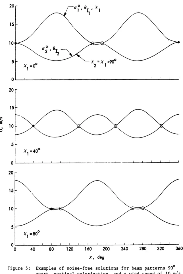
One limitation of this a -to-wind algorithm is that for a given ao grouping there may be up to four possible wind vector solutions, all with approximately the same wind speed, but with widely varying directions. Figure 5 illustrates this for the ideal case of two orthogonal, noise-free, colocated a measurements of the same

wind. The curves are possible solutions in wind speed (U)-azimuth angle (X) space for particular values of backscatter (aO ) and incidence angle (O8). Wind solutions are found at the curve intersections and this case shows the large variation of directions and small range of wind speeds for the different possible solutions. As shown, a 900 separation in azimuth yields the most distinct intersections. Noisy measurements further complicate this process, since the intersections are then spread over a larger area. These direction aliases cannot be removed without further processing, usually requiring some independent knowledge of the wind field. Future scatterometers will help resolve this ambiguity problem, by adding an additional antenna on each side, reducing the maximum number of solutions to only two, separated by nearly 1800.

SASS performance evaluations

Evaluations of the final SASS wind retrieval algorithms initially indicated that it met the required specifications of ±2 m/s in wind speed and ±200 in wind direction on a synoptic scale. The final results from the SASS workshops were rms differences of 1.3 m/s for a range of 4 to 26 m/s, and 160 for a 00_-to-3600 _{range (Lame and Born,}

1982; Jones et al., 1982). However, these rms values were calculated for a restricted data set that was limited to the particular wind speed range and geographical area of the conventional wind data used for tuning and validation. These statistics do not always accurately reflect performance for other subsets of the data, as discussed in detail by Woiceshyn et al. (1986). Sources of error for the SASS generated winds exist both in the geophysical interpretation of the radar signal and in factors that may contaminate the signal, such as rain, sea surface temperature, and radar polar-ization. Many of these questions were addressed in the scattering theory discussion. An additional point is that the inherent spatial averaging of each SASS footprint may smooth out variations of the small scale turbulent winds (up to 10 m/s) embedded in the footprint area (Brown, 1986). The spatial smoothing may be especially signif-icant for small, intense features, such as thunderstorms. Strong circulation features, such as fronts, cyclones, and hurricanes, also pose a problem, since they generally

_IIIIL_ ~_IYX~ _I~L -- -i~.~ ~- C ----~- LLILCII _I_ ~i~Pr~l l X _ILXXl~i-~*--^XI~1)--LI~L ~1- l);~.l~ LIII I_-~L--~_ -_YY---L-n_-YIIL~L~-BYII ~ .(-- ~-)-..I~LL*-- 11I

violate the steady state conditions assumed in the a" -to-U algorithms. Differences in wind retrieval system behavior across a front are evident in the changed charac-ter of the scatcharac-teromecharac-ter signal across the front (Brown, 1983). Adjustments to the wind retrieval system are needed to more fully account for these flow features, most likely as parameterizations that can be incorporated into the steady state algorithms

(Brown, 1986).

Various evaluations of the SASS data have identified problems with different aspects of the wind retrieval algorithms. Woiceshyn et al. (1986) use intercomparisons of horizontally and vertically polarized SASS data and comparisons between in situ and SASS winds to demonstrate the inadequacy of the power law relation at all observed wind speeds and incidence angles. This stems from the tuning of the data to the limited range of conditions observed in the "surface truth" experiments and to the inability of a single power law to model the difference in surface roughness over two distinct wind regimes. Woiceshyn et al. (1986) discuss other problems, including the inaccuracy of the SASS winds at low wind speeds. The combination of a sum-of-squares inversion technique and the signal from noise subtraction process may yield negative backscatter values for light winds (Pierson et al., 1986). Using a power law assumption with this inversion process means that the negative values must be discarded, causing a considerable loss of information at lower wind speeds. A better option may be to use a maximum likelihood estimation inversion that will make use of all the data (Pierson et al., 1986). Preliminary work on a new scatterometer wind extraction system that removes many of these biases in the SASS model is presented in Woiceshyn et al. (1984). A careful statistical analysis of the original SASS winds

by Wentz et al. (1984, 1986) also revealed several systematic errors in the SASS data.

They found that horizontally polarized backscatter signals yielded winds that were biased high relative to those from vertically polarized backscatter returns, a cross-swath wind gradient error was introduced from an incorrect a' vs incidence. angle relation, low signal-to-noise ratio a' values were discarded - so low winds were biased high and data gaps existed for areas of light winds, and the SASS winds were biased high by approximately 1 m/s relative to conventional winds. Some of these errors are

similar to those discussed by Woiceshyn et al. (1986), but Wentz (1986) retains the power law relation and corrects the model coefficients, rather than choosing another form for the model function. Finally, the question of directional ambiguity in the wind vector solutions has received considerable attention (Wurtele et al., 1982; Peteherych et al., 1984). Several alternatives to the SASS algorithm method have been developed (Hofman, 1982, 1984; Gohil and Pandey, 1985; Woiceshyn et al., 1986; Brown, 1986), and the design of future scatterometers will considerably reduce this alias problem.

SASS data reprocessing

The original SASS wind data, processed with the model function and cell-pairing method described above, is available on Geophysical Data Record (GDR) tapes lo-cated at the Jet Propulsion Laboratory (JPL). The alias problem and other errors discovered in the initial GDR processing, mentioned briefly above, motivated a re-processing of the entire sensor data set. Wentz et al. (1986) reprocessed the entire 96-day data set, binning the backscatter values into 50 km cells oriented perpendicu-lar to the satellite subtrack. These combined a measurements were then inverted to obtain the wind vectors, on both 50 and 100 km grids. The winds were retrieved with an improved oo -to-wind model, based on an assumed Rayleigh wind distribution, rather than tuning to in situ measurements. The model was designed to minimize the systematic errors dependent on polarization or incidence angle identified earlier, and used a single power law relationship, except for an adjustment for the higher nadir winds. Based on climatology, the winds were assumed to be Rayleigh distributed about a mean of 7.4 m/s (Wentz et al., 1984). This statistical approach has several advantages over a tuning approach, including the ability to use all the satellite mea-surements, rather than just those matched with a limited, high-quality conventional data set, and elimination of the problem of matching the different temporal and spa-tial scales of satellite and conventional data. The pre-averaging of the backscatter measurements across larger cells increases the signal-to-noise ratio (SNR) for the final ao value, which is especially useful at low wind speeds. A typical cell in the middle

of the swath contained four aO measurements from each antenna, and SNR increased

by a factor of two (Wentz et al., 1986). These reprocessed winds show more

con-sistency and lower residual errors than the original SASS winds in intercomparisons over different polarizations and incidence angles. A comparison to buoy winds showed good general agreement in wind speed, with a 1.6 m/s rms difference and -0.1 m/s bias, supporting the statistical assumptions made in deriving the new model (Wentz et al., 1986).

The directional ambiguity in the SASS winds was removed by several different methods, both subjective and objective, for various subsets of the original data. Pete-herych et al., (1984) developed a subjective dealiasing method and produced a global, 15-day (6-20 September 1978) set of dealiased SASS winds. Their method is based on procedures described by Wurtele et al., (1982) and Baker et al., (1984), where meteorological analysis and pattern recognition are used to select an alias. Rather than using subjective meteorological analysis to dealias the data, alternative objec-tive techniques have been developed, including those of Hoffman (1982, 1984), Baker et al., (1984), and Yu and McPherson (1984). Atlas et al., (1987), used a modified version of the model of Baker et al., (1984) to objectively dealias the complete 96-day set of reprocessed, 100 km resolution, multiple-solution vectors. Atlas et al., (1987) employed the Goddard Laboratory for Atmospheres (GLA) analysis/forecast system

in an iterative, three-pass procedure, combining conventional data and previously analyzed SASS winds as a first-guess field. These unambiguous SASS wind vectors are subsequently identified as Atlas winds in this paper, to distinguish them from the original GDR winds. They form the principal set of scatterometer winds to be evaluated and compared with conventional wind data in this study.

4. Data description and handling

The initial data set obtained was a subset of the GDR data, supplied by NASA Ocean Data Systems (NODS) at JPL. Figure 6 shows a swath of these winds from SEASAT revolution 184. The alias problem discussed above limited its usefulness, and when the Atlas data set became available it was used, rather than the GDR data, for all subsequent evaluations. As mentioned in Section 3, the Atlas SASS winds are referred to as Atlas winds, in order to distinguish them from the original GDR data and from other sets of SASS wind data. In the preliminary analysis, we removed the directional ambiguity for selected GDR winds subjectively, by comparison of the plotted GDR wind vectors to synoptic weather and pressure maps. The SASS solution in closest agreement with the conventionally derived wind field was selected wherever possible, while those cases where an unambigous solution was not obvious were dropped from further consideration. Due to uncertainties imposed by this rough dealiasing scheme, the GDR winds were most useful in an initial screening of the Atlas winds, rather than as input for further analysis. After basic pattern agreement was established, these winds were most useful in ensuring the proper reading, transfer, and display of Atlas wind vector data. This study concentrates on a one-month subset of the full 96-day record, from 12 August to 10 September 1978, over a portion of the western North Atlantic, from 20-30oN and 40-800_{W. The Atlas data is regularly}

spaced along the satellite subtrack, but it is irregularly spaced on a latitude-longitude grid, and the nature of satellite orbit ground coverage means that data samples in a given area are widely separated in both time and space. Typically, two passes cross the study area, separated by approximately 100 minutes and 2500 km, followed 12 hours later by another two passes, offset in space from the first pair.

Since the primary purpose was to compare scatterometer winds to a conventional wind field, a readily available, suitable conventional wind field was needed. The 6-hour synoptic surface wind analyses provided by the Fleet Numerical Oceanographic Center (FNOC) in Monterey, CA, through the National Center for Atmospheric Research (NCAR), were selected. These winds are generated by combining ship and buoy wind