HAL Id: inserm-00212329
https://www.hal.inserm.fr/inserm-00212329
Submitted on 13 Jun 2008HAL is a multi-disciplinary open access archive for the deposit and dissemination of sci-entific research documents, whether they are pub-lished or not. The documents may come from
L’archive ouverte pluridisciplinaire HAL, est destinée au dépôt et à la diffusion de documents scientifiques de niveau recherche, publiés ou non, émanant des établissements d’enseignement et de
Coding of movement- and force-related information in
primate primary motor cortex: a computational
approach.
Emmanuel Guigon, Pierre Baraduc, Michel Desmurget
To cite this version:
Emmanuel Guigon, Pierre Baraduc, Michel Desmurget. Coding of movement- and force-related infor-mation in primate primary motor cortex: a computational approach.. European Journal of Neuro-science, Wiley, 2007, 26 (1), pp.250-60. �10.1111/j.1460-9568.2007.05634.x�. �inserm-00212329�
Editor: M. Rushworth
Coding of movement- and force-related
information in primate primary motor
cortex: A computational approach
Emmanuel Guigon 1
, Pierre Baraduc 2
, Michel Desmurget 2 1
INSERM U742, ANIM
Université Pierre et Marie Curie (UPMC – Paris 6) 9, quai Saint-Bernard, 75005 Paris, France
2 Centre de Neurosciences Cognitives, CNRS UMR 5229,
67, Bd Pinel, 69675 Bron, France
Running head: Optimal motor control
Correspondence to: Emmanuel Guigon INSERM U742, ANIM U.P.M.C., Boîte 23 9, quai Saint-Bernard 75005 Paris, France Fax: 33 1 44 27 34 38 Tel: 33 1 44 27 34 37 Email: [email protected]
27 pages / 10 figures / 0 table / 20 equations
Number of words: whole = 8247 / abstract = 162 / introduction = 423
Keywords: Neuron; Force; Muscle; Control; Computer
HAL author manuscript inserm-00212329, version 1
HAL author manuscript
Abstract
Coordinated movements result from descending commands transmitted by central motor systems to the muscles. Although the resulting effect of the commands has the dimension of a muscular force, it is unclear whether the information transmitted by the commands concerns movement kinematics (e.g. position, velocity) or movement dynamics (e.g. force, torque). To address this issue, we used an optimal control model of movement production which calculates inputs to motoneurons which are appropriate to drive an articulated limb toward a goal. The model quantitatively accounted for kinematic, kinetic and muscular properties of planar, shoulder/elbow arm reaching movements of monkeys, and reproduced detailed features of neuronal correlates of these movements in primate motor cortex. The model also reproduced qualitative spatio-temporal characteristics of movement- and force-related single neuron discharges in nonplanar reaching and isometric force production tasks. The results suggest that the nervous system of the primate controls movements through a muscle-based controller which could be located in the motor cortex.
Motor control is central to executive functions of the nervous system. It guarantees that planned actions are efficiently translated into appropriate limb displacements. A striking feature of this translation from “ideas of motion” to “mechanical motion” is the paradoxical contrast between the apparent easiness with which movements are performed on the one hand, and the complexity of Newtonian dynamics, and the existence of multiple levels of redundancy, on the other hand (Bernstein, 1967). Since the time of Bernstein, this paradox has been copiously documented and solutions have been proposed to explain how the nervous system can solve such a challenging problem (Bullock & Grossberg, 1988; Uno et al., 1989; Kalaska & Crammond, 1992; Harris & Wolpert, 1998; Todorov & Jordan, 2002; Guigon et
al., 2007). Yet the central issue of the nature of neural control signals (NCSs) that flow from
central motor systems to the periphery during coordinated movements remains open and hotly debated (Kalaska et al., 1989; Caminiti et al., 1991; Fetz, 1992; Feldman & Levin, 1995; Georgopoulos, 1996; Kakei et al., 1999; Georgopoulos & Ashe, 2000; Moran & Schwartz, 2000; Todorov, 2000, 2003; Scott, 2005; Aflalo & Graziano, 2006).
A common method to address this issue is to record NCSs in vivo, e.g. using single unit recordings in primary motor cortex (M1) and spinal cord of behaving animals (monkeys), and to perform a correlation analysis in order to reveal preferential relationships between discharge rates and parameters of motor behavior (e.g. direction of movement, velocity, joint torques; Evarts, 1968; Georgopoulos et al., 1982; Kalaska et al., 1989; Moran & Schwartz, 1999). This method has revealed a large repertoire of discharge patterns as well as a large repertoire of correlations which were thought to reflect sometimes kinematic (direction, velocity), sometimes dynamic (forces) representations of motor acts. However, these correlations were time-varying and complex (Ashe & Georgopoulos, 1994; Fu et al., 1995),
and were in general contaminated by real or apparent covariations among parameters (Mussa-Ivaldi, 1988; Todorov, 2000; Scott, 2005). Furthermore, as correlations do not imply causality, neurophysiological data are not sufficient to draw firm conclusions on this issue. A complementary approach is to define the requisite characteristics of neural control signals based on a model of motor control and to compare requisite and actual properties of these signals (Lan, 1997; Bullock et al., 1998; Todorov, 2000; Haruno & Wolpert, 2005). Here, we exploit an optimal control model which quantitatively accounts for kinematic and dynamic properties of redundant manipulators (Guigon et al., 2007) to address the nature of neural control signals generated by the nervous system to control arm reaching movements.
Materials and Methods
Scope of the model
To properly ascertain the contribution of neural activities to movement control, it is necessary to consider neural and movement data simultaneously. An appropriate animal (monkey) model of this situation is obtained using a mechanical exoskeleton which puts constraints on the degrees of freedom (DOF) involved in the movement (Scott et al., 2001; Graham et al., 2003; Kurtzer et al., 2006). In this case, the mechanical apparatus can be represented by a planar two-joint arm. In other studies of interest (Caminiti et al., 1991; Sergio & Kalaska, 1998; Kakei et al., 1999; Sergio et al., 2005), the movements involved more than 2 DOF. In theory, the model could be used to address these experiments (Guigon et al., 2007). However, not enough kinematic and kinetic data are available in these studies for a thorough comparison between experimental observations and predictions of the model. Accordingly, we thoroughly and quantitatively addressed the neural control of planar two-joint arm
movements. In this framework, we also reproduced qualitative aspects of motor cortical discharge related to nonplanar arm reaching movements (Sergio & Kalaska, 1998; Sergio et
al., 2005).
The model described in this article is formally identical to the model used in Guigon et al. (2007). Yet the two articles address complementary issues. In the previous article, we described predicted kinematic and dynamic characteristics of upper limb movements. Here, we focus on the nature of the predicted control signals which are responsible for these movements. For clarity, we give below a brief overview of the model, but a thorough presentation can be found in Guigon et al. (2007).
Overview of the model
In a schematic view of motor control, a cortical motor center sends a command to a neuromuscular apparatus (motoneuron + muscle) which generates a force to displace a set of articulated segments. Formally, this series of events can be represented by the action of a
controller upon a controlled object. Mathematically, the behavior of the controlled object can
be described by a state-dependent dynamics
dx/dt = f (x(t),u(t)), (Eq. 1)
where x is the state vector of the object (position, velocity, muscle state, …), and u = {ui}
(1 ≤ i ≤ M, M number of muscles) the control vector (or control signal; CS) transmitted by the controller. A control problem corresponds to the mastering of the controlled object, i.e. find a time series of control u(t) (t in [t0;tf]) in order to satisfy to constraints of a task, e.g.
x(t0) = x0 and ψ(x(tf)) = 0, (Eq. 2)
where function ψ expresses constraints on the final state of the object.
Once the control problem is solved, the quantities x(t) and u(t) can be analyzed and compared to corresponding quantities obtained in experimental studies: position/velocity to movement kinematics, force/torque to movement dynamics, control to cortical activity. In the framework of this study, an appropriate controller should meet the following requirements: 1. to provide a unique solution in the face of spatial, temporal, kinematic and muscular redundancy; 2. to provide a solution which has realistic kinematic characteristics. We have shown previously that a controller which chooses, among solutions to Eqs. 1 and 2, the unique solution that minimizes overall control magnitude (E, effort)
E2
=
∫
[t0;tf] ||u(t)|| 2dt, (Eq. 3)
where ||u(t)|| is the norm of vector u, comply with these requirements (Guigon et al., 2007). Technically, u is the solution of an optimal control problem. Since the focus of this article is the issue of the nature of neural control signals which are elaborated by the nervous system to produce coordinated movements, we do not intend here to show that this controller is more realistic or efficient than other controllers. The fact that results described below could be obtained with other controllers is not at all detrimental to our purpose.
In general, Eq. 1 includes both dynamic (inertial, velocity-dependent) and static (elastic, gravitational) forces. A series of arguments (reviewed in Guigon et al., 2007) suggests that the nervous systems processes the two types of force separately (separation principle), i.e.
u(t) = udyn(t) + ustat(t),
where udyn(t) is the solution to the optimal control problem without static forces, and ustat(t)
compensates for applied static forces. In the following, we only address the nature of dynamic
CSs, in the absence of static forces. In the following u corresponds to udyn.
The controller is described here as an open-loop controller. However, it should be noted that the model is affiliated with a principled approach to motor control which states that feedback is a necessary component of an appropriate neural controller (Guigon et al., 2007). Thus the controller can be considered as an optimal feedback controller, i.e. a controller which calculates the appropriate command to reach a goal for any estimate of the state of the controlled system (see also Todorov, 2004; Scott, 2004). Such a model can work properly in the presence of noise in sensory and motor pathways, and perturbations on limb or target position (Todorov & Jordan, 2002; Guigon et al., 2007). In practice, the feedback component remains hidden since neither perturbations nor noise were introduced in the simulations. The results described below can be considered as mean data over noise distributions.
Controlled object
The controlled object was a planar, two-joint (shoulder, elbow) arm actuated by two pairs of monoarticular muscles and one pair of biarticular muscles (Fig. 1A). For each muscle, actual force F was calculated following Zajac (1989) and Brown et al. (1996). We used
F = Γ × PCSA × Fa (u) × (FV × FL + FP) (Eq. 4)
where
- u is a control input (component of vector u for the corresponding muscle), - Γ is a tension scaling factor,
- PCSA is the physiological cross-sectional area,
- Fa is a unitless quantity derived from muscle input,
Fa = η(a)
υ da/dt = - a + e (Eq. 5) υ de/dt = - e + u
where a and e are muscle activation and excitation, η(z) = [z]+
([z]+
= z if z > 0 otherwise [z]+ = 0), υ is a parameter;
- FP reflects passive forces
FP = c2 {exp[k2(L-Lr2}]-1}
where L is the normalized muscle length (the normalization factor is the length L0 at which
maximal isometric force is generated), c2, k2, Lr2 are parameters;
- FL and FV are related to force-length and force-velocity curves of the muscle,
FL = exp{-[(L
β-1)/ω]ρ}
FV = (b1-a1V)/(V+b1) if V < 0 (shortening muscle)
FV = (b2-a2V)/(V+b2) if V > 0 (lengthening muscle)
where V is the normalized muscle velocity (in units of L0/s), β, ω, ρ, a1, b1, a2, b2 are
parameters. The quantity FV × FL + FP is plotted as a function of L and V in Fig. 1B. (Fig. 11B
in Brown et al., 1996).
The muscle forces were translated into joint torques according to
Tsh = γsh FL × Fsh FL - γsh EX × Fsh EX + γbish FL × Fbi FL - γbish EX × Fbi EX Tel = γel FL × Fel FL - γel EX × Fel EX + γbiel FL × Fbi FL - γbiel EX × Fbi EX where γxx YY
are the moment arms of the muscle, with xx = {sh, el, bi, bish, biel} and YY = {FL, EX}, sh = shoulder, el = elbow, bi = biarticular, FL = flexor, EX = extensor.
The controlled object contains two elements which are though to play an important role in motor control: 1. force-length and force-velocity relationships in muscles (Todorov, 2000); 2. biarticular muscles (van Bolhuis et al., 1998). To address the influence of these elements in the framework of this study, we considered two modified versions of the model: 1. a model (NOLV) without force-length and force-velocity relationships in the muscles (i.e. F = Γ ×
PCSA × Fa in Eq. 4); 2. a model (NOBI) without biarticular muscles (γbi*
*
= 0).
Neural control signals
The control problem (Eqs. 1,2,3) was modified to account for the fact that there are many more neurons potentially involved in motor commands than muscles. We assumed that 1. the number s of control signals was larger than the number M of muscles; 2. each control signal was defined by a fixed synergy of muscles (Eq. 7); 3. the s synergies were uniformly distributed in muscular space (Eq. 7). Formally, the problem was similar to the problem defined by Eqs. 1,2,3 with the following change. The goal was to find minimum control U(t) = {Uj(t)} (1 ≤ j ≤ s), i.e the unique solution that minimizes
E2
=
∫
[t0;tf] ||U(t)|| 2dt, (Eq. 6)
and is appropriate to displace the articulated segments between given initial and final
positions, the muscular control vector u(t) = {ui(t)} (1 ≤ i ≤ M) being defined by
ui(t) =
Σ
j=1..s βij Uj(t), (Eq. 7)where βij are random coefficients drawn from a uniform distribution in [-1;1]. The control
signals {Uj(t)} are called neural control signals (NCSs).
Tasks
To simulate arm movements, the torques (Tsh,Tel) were translated into displacements using the
dynamics of the articulated segments (Newtonian dynamics; Guigon et al., 2007). The control vector was
u(t) = [u1,u2,u3,u4,u5,u6]
i.e. the control for the shoulder flexor, shoulder extensor, elbow flexor, elbow extensor, biarticular flexor, biarticular extensor, in this order. For a movement task, the state vector was
x(t) = [q1,q2,dq1/dt,dq2/dt,a1,a2,a3,a4,a5,a6,e1,e2,e3,e4,e5,e6],
where q1 and q2 are the shoulder and elbow angles, dq1/dt and dq2/dt the shoulder and elbow
velocities. The boundary conditions (Eq. 2) were the initial and final arm postures with zero initial and final velocity, activation and excitation (i.e. x(t0) = x0 and ψ = x(tf) - xf), where
x0 = [q10,q20,0,0,0,0,0,0,0,0,0,0,0,0,0,0]
and
xf = [q1f,q2f,0,0,0,0,0,0,0,0,0,0,0,0,0,0].
To simulate isometric force production, the torques were translated into endpoint force (Φ) using
T = J(q)T
Φ, where T = [Tsh Tel]
T
, and J(q) is the Jacobian matrix of the kinematic transformation at position q = [q1 q2]
T
. The state vector was
x(t) = [a1,a2,a3,a4,a5,a6,e1,e2,e3,e4,e5,e6].
A force trajectory was specified by initial and final forces (Φ0 and Φf). The boundary conditions were x0 = [a10,a20,a30,a40,a50,a60,e10,e20,e30,e40,e50,e60] and ψ(x(tf)) = T(tf) - Tf where Tf = J(q) T Φf. For simulations, (q1,q2) = (q10,q20).
Solution to the optimal control problem
The problem defined by Eqs. 1,2,3 or Eqs. 1,2,6,7 was solved numerically using a gradient method (Bryson, 1999; Guigon et al., 2007). The results were obtained as x(tk), u(tk), (or
U(tk)) for
tk = t0 + (tf – t0)k/n (Eq. 8)
with k = 0 … n, and n = 50.
Data analysis
The CSs and NCSs can be considered as inputs to motoneurons (Eq. 4), and could correspond to activities in subsets of cortical and spinal neurons. They were analyzed as if they were the discharge of motor cortical neurons, i.e. by quantifying their directional tuning using regression analysis (Georgopoulos et al., 1982). For each NCS, preferred directions (PDs)
were calculated at each timestep tk (0 ≤ k ≤ n). The main PD was defined as PD(t = t0).
Population vectors were calculated following classical techniques. Bimodal distributions were frequently encountered, and were quantified by a preferred axis as defined by principal
component analysis. Electromyographic (EMG) activity was defined as [e]+
(e, excitation; Eq. 5).
Parameters and comparison with experimental data
The model was built for a direct comparison with experimental data in monkeys (Scott et al., 2001; Graham et al., 2003; Kurtzer et al., 2006). Thus, a number of parameters were directly
taken monkey data. Biomechanical parameters (segment inertia I in kg m2
, mass m in kg, center of mass cof in % of the length, length L in m) were taken from Cheng & Scott (2000) for Macaca mulatta. Indexes 1 and 2 are used for upper arm and forearm, respectively. We used I1 = 0.00126, m1 = 0.699, cof1 = 0.5, L1 = 0.144, I2 = 0.00621, m2 = 0.781, cof2 = 0.375,
L2 = 0.257. Muscular parameters were taken from Brown et al. (1996): c2 = -0.02 , k2 = -18.7,
Lr2 = 0.79, β = 2.3, ω = 1.26, ρ = 1.62, a1 = 0.17, b1 = -0.69, b2 = 1.8, a2 = pL 2
+ qL + r, p = -5.34, q = 8.41, r = -4.7. Muscle time constant was υ = 0.05 s (van der Helm & Rozendaal, 2000). The moment arms (Graham & Scott, 2003) are shown in Fig. 1C.
Parameters which are less well defined are the tension scaling factor Γ (Buchanan, 1995), and the PCSAs which depend on the muscles which are actually involved at a given
articulation. We chose Γ = 35 N/cm2
, and the PCSAs were used as free parameters, and were adjusted according to the following criteria: 1. Each PCSA is in a reasonable range (1-15 cm2
); 2. Movement trajectories have a direction-dependent curvature (Fig. 1 in Graham et al., 2003); 3. Spatial selectivity of the muscles is as close as possible as that described by Kurtzer
et al. (2006). Yet, as the model entails a number of simplifications, we though that the search
of an exact fit of the data would be meaningless. Thus, we used a set of PCSAs which provide
a good description of experimental observations. The PCSAs (in cm2
) were (for shFL, shEX,
elFL, elEX, biFL, biEX): 10, 10, 11, 11, 9.9, 9.9.
For comparison between outcomes of the model and experimental data, we either reproduce an original figure, or indicate in the text a reference to one or more published figures.
Results
Properties of planar, 2-DOF reaching movements
Mechanical, muscular and neural characteristics of planar, 2-DOF reaching movements have been thoroughly studied by Scott et al. (2001), Graham et al. (2003), and Kurtzer et al. (2006) (noted Scott, Graham and Kurtzer below). In these experiments, monkeys performed radial reaching movements toward 16 targets. Movement amplitude was 6 cm, and movement duration was ~600 ms (576 ms in Scott; Figs. 1,2 in Graham; Figs. 1,2 in Kurtzer). Initial posture was ~(30°,90°) in Graham and Kurtzer (Fig. 2C in Graham; p 3221 in Kurtzer), but was not reported in Scott. In this latter case, we used (30°,80°) which provides a good fit to the data. We simulated similar movements with the model, and we obtained movement kinematics (trajectories), movement kinetics (torques, power), muscular activities and neural control signals.
Kinematics and kinetics
Trajectories are shown in Fig. 2A, and Fig. 1A,B,C in Graham for comparison. Note that the model accounted for directional variations in movement curvature (see also Guigon et al., 2007). The model also reproduced the anisotropy in motion at shoulder and elbow joints (Fig. 2B,C,D,E,F; Fig. 3A,C,D,E,F in Graham, Fig. 2C in Kurtzer). The kinetic data reported
by Graham concerned active torques, i.e. the combination of passive torques generated at shoulder and elbow and voluntary muscular torques. Active torques were obtained with the model by subtracting modeled passive torques (from Fig. 3C,D in Graham) from actual torques generated by the controller. The results are shown in Fig. 3. The model reproduced directional variations in peak active torque (Fig. 3A,B,C; Fig. 5A,B,C in Graham, Fig. 2C in Kurtzer) and peak joint power (Fig. 3D,E,F; Fig. 8A,B,C in Graham). A difference between the experiment and the model was found for the spatio-temporal profile of active shoulder torques (Fig. 3B; Fig. 5B in Graham). A possible reason for this difference is related to approximations in the representation of the passive torques. Similar results were obtained with the modified models (NOLV and NOBI).
Muscular activity
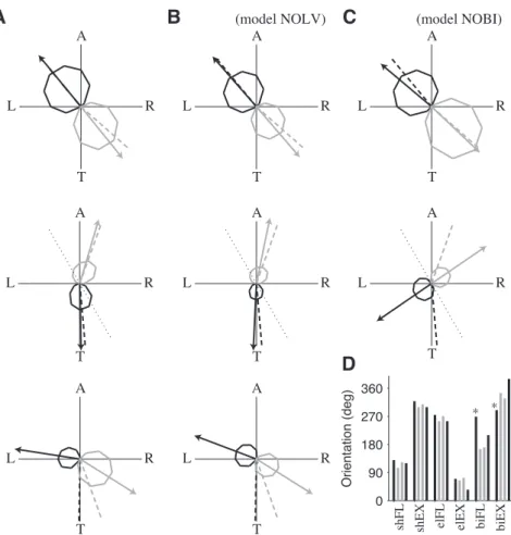
Peak muscular activities varied with movement direction (Fig. 4A; Fig. 6 in Kurtzer). The monoarticular muscles behave as found experimentally [130°-309° (model) vs 130°-319° (Kurtzer) axis for the shoulder muscles; 271°-73° (model) vs 275°-70° (Kurtzer) axis for the elbow muscles]. We could not reproduce the observations of Kurtzer on the activities of the biarticular muscles. The origin of this discrepancy is unclear. We first note that the search over PCSAs has never lead to activities of the biarticular muscles as predicted by Kurtzer. Furthermore, similar results were reported by Li (2006) with a closely related model (her Fig. 5.7; see also Todorov & Li, 2005). Thus our results could hardly be ascribed to some errors in the simulations of the model. To deepen this issue, we have plotted the preferred axis of the 6 muscular types obtained by Kurtzer in monkeys, by Li (2006) and by us in an optimal control model, and by Welter & Bobbert (2002) in humans (Fig. 4D). We observed that the tuning of the monoarticular muscles is consistent across the studies, but there is a noteworthy
discrepancy between Kurtzer and the other studies for the biarticular muscles (* in Fig. 4D). We also note that the model proposed by Kurtzer to explain their data does not reproduce the tuning of the biarticular muscles (their Fig. 11C). The discrepancy between the model and the data does not prevent the model to explain the characteristics of neural control signals (see below).
Neural control signals
We analyzed the NCSs (s = 500) corresponding to movements from initial posture (30°,80°). We calculated the main preferred direction of each NCS (see Materials and Methods) and the distribution of main PDs over the NCSs. This distribution was anisotropic with a preferred axis along 123-303° (Fig. 5A; 118-298°, Fig. 3 in Scott). The population vector systematically deviated from movement direction (Fig. 5B; Fig. 2A in Scott). We explored the relationship between PD distribution and direction-dependent variations in peak angular velocity, peak joint torque, and peak joint power. The best correlation was found with peak joint power (Fig. 5D; Fig. 4 in Scott).
The PD distribution remained anisotropic for different orientations of the arm and the forearm, and its orientation rotated with both shoulder and elbow angles (Fig. 6A,B). These results can be considered as predictions since the corresponding experiment has not been performed with a mechanical exoskeleton. Yet, they are consistent with results obtained with other kinematic chains (Caminiti et al., 1991; Kakei et al., 1999).
Similar results were obtained with the modified models (NOLV and NOBI). However, the correlations with peak joint power were weaker (not shown), and the PD distribution rotated more steeply with elbow angle (Fig. 6B).
Other movements
Complementary information on the nature of NCSs can be found in other studies which analyzed the temporal structure of motor cortical discharges during reaching movements and isometric force production (Sergio & Kalaska, 1998; Sergio et al., 2005). However, as neither kinematics nor kinetics were quantitatively described in these studies, we only addressed qualitative features of neural discharges. Furthermore, as we found that all the NCSs were qualitatively similar, we only analyzed the 6 CSs (one per muscle).
The raw temporal profile of the shoulder extensor control is shown in Fig. 7 for movements in 8 directions (Fig. 7, center). The control had: 1. an early phasic component followed by a depression for the rightward/downward movements; 2. a delayed phasic component for a movement in the opposite directions. We note that quantitatively similar results were obtained with the NOLV model (Fig. 7, gray lines). Similar temporal profiles were found for the other muscles, each with its preferred directional tuning (not shown). For comparison with experimental data, we have replotted the control for the shoulder extensor in a different format which can be read as a mean discharge frequency (Fig. 8A). Data from single unit recording in primate primary motor cortex are reproduced (Fig. 1 in Sergio & Kalaska, 1998; Fig. 8B). Visual inspection revealed a close correspondence between real and simulated profiles although a difference was visible at the end of the movement (see Discussion). We note that the large phasic transient near the end of the movement (Fig. 7; Fig. 8A) is due a strict boundary condition (Eq. 2): the movement must finish at a given time and position. This type of boundary condition was chosen for simplicity, but requires large controls to guarantee the exact fulfillment of spatial and temporal constraints. Yet real movements do not in general terminate abruptly, but end up smoothly, e.g. with oscillations.
A more realistic movement could be obtained in the presence of noise. In this case, estimated limb position is in general different from actual limb position so a nonzero residual error should always be present to drive movement corrections. This case is illustrated in Fig. 1D of Guigon et al. (2007).
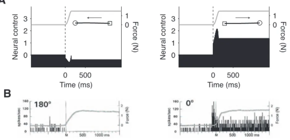
For comparison, we applied the model to the production of isometric forces in different directions. Since the calculated control signals are related to dynamic forces, they are not responsible for static force exertion after the dynamic period. To obtain more realistic control signals, we added a static component necessary for the maintenance of a steady final force. For a 150-ms force increase from 0 to 1.5 N, the temporal profile of the shoulder extensor control signal had a phasic excitation for a rightward-directed force (Fig. 9A, right) and a phasic inhibition for a leftward force (Fig. 9A, left). Data from single unit recording in primate primary motor cortex are reproduced (Fig. 1 in Sergio & Kalaska, 1998; Fig. 9B).
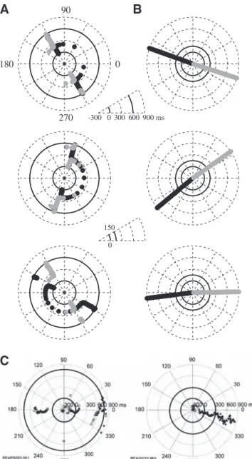
Preferred directions of the CSs were calculated every 10 ms and displayed in a circular plot (Fig. 10). In the movement task (Fig. 10A; from top to bottom, sh, el, bi; black circle: flexor;
gray circle: extensor), the PD reverted during the movement. In contrast, the isometric
controls did not revert their PDs (Fig. 10B). For comparison, data from Sergio & Kalaska (1998) are reproduced in Fig. 10C.
Discussion
The present article describes a model-based approach to the nature of neural control signals generated by the nervous system of monkeys to control arm movements. The model reproduces detailed features of movement kinematics and kinetics, and quantitative characteristics of single neuron and population discharges in primate motor cortex. The
results support the idea that 1. the motor system controls movement using a muscle-based controller; 2. this controller could be located in the motor cortex.
Nature of the model
The model is an optimal controller, i.e. a controller which calculates appropriate control signals to displace a controlled object using a complete knowledge of the properties of the object (here, the dynamics of the arm and the characteristics of the muscles), and an optimality criterion. Recent reviews have thoroughly advocated this type of model to address behavioral and neural characteristics of goal-directed movements (Todorov, 2004; Scott, 2004). We refer the reader to these reviews for a detail discussion of optimal control models. The present model is not fundamentally different from previous models which applied optimal control techniques to determine the spatio-temporal nature of command signals which should enter a neuromuscular system to drive a limb toward a goal (Happee, 1992; Lan & Crago, 1994; Lan, 1997; Harris & Wolpert, 1998; Haruno & Wolpert, 2005; Todorov & Li, 2005; Li, 2006). A common result of these models is that optimal control of a low-pass filtering force generating system leads to reasonably realistic EMG and neural control signals. The originality of this work is not to describe a new, more efficient model, but to deepen our understanding of neural information processing in motor cortex using a model-based approach, which proves that observed discharge characteristics of single neurons and populations recorded during movements in M1 can be quantitatively explained by observed characteristics of the movements. In fact, previous models have addressed properties of neurons, but not properties of limb movements (Lan, 1997; Bullock et al., 1998; Todorov, 2000; Haruno & Wolpert, 2005; Trainin et al., 2007).
Limitations
There are at least three limitations to the present model. First, although the model appropriately produces the expected results, the issue of its validity in a broader framework remains open. The model was actually tested in various conditions, and was found to be consistent with experimental observations (Guigon et al., 2007). Yet some data, e.g. highly nonsymmetric velocity profiles, cannot be explained by the model. Second, the way optimal feedback control can be computed by brain circuits remains elusive. A third and related limitation is the absence of relationship between the computational processes advocated by the model and organizational features of the motor cortex (connectivity, intrinsic properties, …). The two latter issues raise the problem of neural information processing subserving motor control. This problem has been addressed for initial directional commands of reaching movements (Baraduc et al., 2001), but remains open for the whole spatiotemporal commands.
Motor cortical physiology
Single cell recordings in M1 have revealed a large repertoire of discharge patterns. In fact, the greater part of movement parameters, ranging from exerted force (low-level muscle control) to serial order of stimuli (cognitive motor control) have been found to influence the discharge of motor cortical neurons (Ashe, 1997; Georgopoulos, 2000). This paradox is hotly debated (Georgopoulos & Ashe, 2000; Moran & Schwartz, 2000; Todorov, 2000). A central issue of the debate is the interpretation of correlation analyses which are used to quantify neuronal activities. For instance, Todorov (2000) defends the view that M1 neurons calculate muscular activation patterns, and suggests that many correlations between kinematic quantities and neural discharges in M1 can be explained by this hypothesis (i.e. they are artifacts). In this
framework, a series of studies by Scott and collaborators have attempted to circumvent the weakness of correlation analysis (Scott et al., 2001; Graham et al., 2003; Kurtzer et al., 2006). They reported a systematic description of planar two-joint arm movements and neural correlates of their execution. They found that anisotropic characteristics of movement dynamics and muscular selectivities were associated with a similar anisotropy in neural selectivities. Our model reproduces a similar relationship between mechanical, muscular and neural quantities, and supports the contention of Scott of a tight link between neural populations in M1 and the motor apparatus. The model further shows that the spatio-temporal profile of the NCSs is qualitatively similar to the activity in a subpopulation of motor cortical neurons (located primarily in caudal M1) whose discharge tightly follows the time course of required task dynamics (Sergio & Kalaska, 1998; Sergio et al., 2005). Taken together, these results suggest that a subset of M1 neurons could actively participate to a muscle-based representation of movements (Todorov, 2000, 2003; Sergio et al., 2005). Although a number of arguments concur to this conclusion (Scott, 1997; Todorov, 2000, 2003), our model provides the first realistic demonstration that muscle-based coding can account simultaneously for movement kinematics, movement kinetics, EMGs, and cortical discharges. If our conclusions are correct, the origin and function of other types of neuron (e.g. those related to visuospatial and kinematic representations of movements) remain to be explained. There are at least two hypotheses. The first is related to the idea of sensorimotor
transformations (Kalaska & Crammond, 1992; Scott, 2005). The assumption is that the
nervous system performs sequential operations which progressively translate spatial information on the goal of the movement into appropriate commands, going through kinematic, dynamic, and muscular stages. In this case, quantities related to desired movement
kinematics, in particular desired movement velocity, should be found in M1 (Moran & Schwartz, 1999). This explanation relies on the questionable idea that motor control is based on trajectory tracking (Todorov & Jordan, 2002; Guigon et al., 2007). The second hypothesis ensues from the model. As discussed in the Materials and Methods, the controller can be considered as an optimal feedback controller, i.e. an optimal controller coupled with a state estimator. We have described properties of the signals elaborated by the controller. Yet other signals should be available to indicate the goal and the estimated state. This latter signal should convey information related to predicted position, velocity, force, … Such a predictive (rather than desired) signal could be a source of kinematic information in motor cortex. For instance, cortical velocity signals have been described in M1 which lead actual velocity by 120-150 ms (Moran & Schwartz, 1999; Wang et al., 2007). As the control signals reported in other studies lead movement onset by 100-200 ms (Kalaska et al., 1989; Sergio & Kalaska, 1998; Sergio et al., 2005), it is possible that the velocity signals derive from the control signals through a forward model. However, these data could also be interpreted to support the presence of a desired velocity signal.
Todorov (2000) has proposed that the dependence of muscle force on length and velocity has a substantial influence on neural information processing in motor cortex. Kurtzer et al. (2006) have suggested that these intrinsic muscular properties are necessary to account for the directional tuning of muscular activities. Our model does not concur with these ideas. First, the temporal profile of our control signals did not resemble a velocity profile (Fig. 7; Fig. 2 in Todorov, 2000). In fact, low-pass filtering renders the control signals much more “phasic” than velocity, even in the presence of a force/velocity relationship in the muscles. Second, muscular tuning was only weakly influenced by force/length and force/velocity relationships
(Fig. 4).
According to the separation principle (Guigon et al., 2007), a complete motor command involves both a static and a dynamic component. Although such components have been observed experimentally in M1 (Cheney & Fetz, 1980; Kalaska et al., 1989; Kurtzer et al., 2005), the discharge of many motor cortical neurons appears to carry simultaneously static and dynamic commands (Cheney & Fetz, 1980; Kalaska et al., 1989; Sergio & Kalaska, 1998; Kurtzer et al., 2005; Sergio et al., 2005). For instance, phasic-tonic neurons recorded by Sergio & Kalaska (1998) have an early component that could be related to the control of dynamic forces (compare Fig. 8A and 8B), and a late component that could be related to the maintenance of posture against a steady force. In fact, Sergio & Kalaska (1998) have found phasic, tonic, and phasic-tonic neurons in equal proportions (~30%), and it is possible that their phasic neurons (not described in detail) are closer to our NCSs than the phasic-tonic neurons. In this case, the phasic and tonic neurons would represent the actual dynamic and static commands as defined by the model. This issue remains to be tested experimentally.
Models of motor control
The debate on the nature of motor cortical representations of movement is part of a more general debate on the nature of motor controllers in the brain (Kawato, 1999; Ostry & Feldman, 2003; Todorov, 2003). On the one hand, position control models exploit viscoelastic properties of muscles and peripheral reflex loops to define limb movements as a series of stable equilibrium postures (Bizzi et al., 1992; Feldman & Levin, 1995). The corresponding descending commands can be viewed as kinematic signals as they need not take into account biomechanical or muscular characteristics of the moving limb (Flanagan et
al., 1993; Georgopoulos, 1996). By construction, the temporal profile of these commands is
monotonic. Computer simulations have shown that triphasic EMG patterns can be obtained from monotonic commands that act to modify the recruitment threshold of muscles rather than the force developed by the muscles (St-Onge et al., 1997; Suzuki & Yamazaki, 2005). On the other hand, force control models have been developed, based on the idea that the nervous system explicitly computes time-varying control signals to achieve a desired movement (Kawato et al., 1987; Uno et al., 1989; Todorov, 2000; Franklin et al., 2003). Although this type of model has been questioned based on the posture/movement paradox (Ostry & Feldman, 2003), it has proven highly efficient to account for a large range of characteristics of motor control (trajectory formation, EMG). The force control models predict that the neural control signals should have nonmonotonic (acceleration-like, torque-like, EMG-like) profiles. The present model, which is affiliated to the force control models (in the sense that the control signals are directly transmitted to a force-generating system), shows that the predicted nonmonotonic NCSs are quantitatively related to the spatio-temporal characteristics of a population of motor cortical neurons. There is no corresponding study of the control signals predicted by position control models and their relationship to cortical physiology. In particular, the origin and role of nonmonotonic discharge patterns in the framework of position control models remain unclear (Todorov, 2003). Although our model cannot directly settle the controversy between force and position control, it gives a physiological basis to the force control models, and contributes to a series of arguments which support these models (Kawato, 1999; Todorov, 2000, 2003; Guigon et al., 2007).
Acknowledgments
We thank Marc Maier for fruitful discussions.
References
Aflalo, T.N. & Graziano, M.S.A. (2006) Partial tuning of motor cortex neurons to final posture in a free-moving paradigm. Proc. Natl. Acad. Sci. U.S.A., 103, 2909-2914.
Ashe, J. (1997) Force and the motor cortex. Behav. Brain Res., 87, 255-269.
Ashe, J. & Georgopoulos, A.P. (1994) Movement parameters and neural activity in motor cortex and area 5. Cereb. Cortex, 4, 590-600.
Baraduc, P., Guigon, E. & Burnod, Y. (2001) Recoding arm position to learn visuomotor transformations. Cereb. Cortex, 11, 906-917.
Bernstein, N. (1967) The co-ordination and regulation of movements. Pergamon Press, Oxford.
Bizzi, E., Hogan, N., Mussa-Ivaldi, F.A. & Giszter, S. (1992) Does the nervous system use equilibrium-point control to guide single and multiple joint movements? Behav. Brain Sci., 15, 603-613.
Brown, I.E., Scott, S.H. & Loeb, G.E. (1996) Mechanics of feline soleus: II. Design and validation of a mathematical model. J. Muscle Res. Cell. Motil., 17, 221-233.
Bryson, A.E. (1999) Dynamic Optimization. Prentice Hall, Englewood Cliffs, NJ.
Buchanan, T.S. (1995) Evidence that maximum muscle stress is not a constant: Differences in specific tension in elbow flexors and extensors. Med. Eng. Phys., 17, 529-536.
Bullock, D. & Grossberg, S. (1988) Neural dynamics of planned arm movements: Emergent invariance and speed-accuracy properties during trajectory formation. Psychol. Rev., 95, 49-90.
Bullock, D., Cisek, P. & Grossberg, S. (1998) Cortical networks for control of voluntary arm
Cheney, P.D. & Fetz, E.E. (1980) Functional classes of primate corticomotoneuronal cells and their relation to active force. J. Neurophysiol., 44, 773-791.
Caminiti, R., Johnson, P.B., Galli, C., Ferraina, S. & Burnod, Y. (1991) Making arm movements within different parts of space: The premotor and motor cortical representation of a coordinate system for reaching to visual targets. J. Neurosci., 11, 1182-1197.
Cheng, E.J. & Scott, S.H. (2000) Morphometry of Macaca mulatta forelimb. I. Shoulder and elbow muscles and segment inertial parameters. J. Morphol., 245, 206-224.
Evarts, E.V. (1968) Relation of pyramidal tract activity to force exerted during voluntary movement. J. Neurophysiol., 31, 14-27.
Feldman, A.G. & Levin, M.F. (1995) The origin and use of positional frames of reference in motor control. Behav. Brain Sci., 18, 723-744.
Fetz, E.E. (1992) Are movement parameters recognizably coded in the activity of single neurons? Behav. Brain Sci., 15, 679-690.
Flanagan, J.R., Ostry, D.J. & Feldman, A.G. (1993) Control of trajectory modifications in target-directed reaching. J. Mot. Behav., 25, 140-152.
Franklin, D.W., Osu, R., Burdet, E., Kawato, M. & Milner, T.E. (2003) Adaptation to stable and unstable dynamics achieved by combined impedance control and inverse dynamics model. J. Neurophysiol., 90, 3270-3282.
Fu, Q.G., Flament, D., Coltz, J.D. & Ebner, T.J. (1995) Temporal encoding of movement kinematics in the discharge of primate primary motor and premotor neurons. J.
Neurophysiol., 73, 836-854.
Georgopoulos, A.P., Kalaska, J.F., Caminiti, R. & Massey, J.T. (1982) On the relations between the direction of two-dimensional arm movements and cell discharge in primate
Georgopoulos, A.P. (1996) On the translation of directional motor cortical commands to activation of muscles via spinal interneuronal systems. Cogn. Brain Res., 3, 151-155. Georgopoulos, A.P. (2000) Neural aspects of cognitive motor control. Curr. Opin. Neurobiol.,
10, 238-241.
Georgopoulos, A.P. & Ashe, J. (2000) One motor cortex, two different views. Nat. Neurosci., 3, 963.
Graham, K.M. & Scott, S.H. (2003) Morphometry of Macaca mulatta forelimb. III. Moment arm of shoulder and elbow muscles. J. Morphol., 255, 301-314.
Graham K.M., Moore, K.D., Cabel, D.W., Gribble, P.L., Cisek, P. & Scott, S.H. (2003) Kinematics and kinetics of multijoint reaching in nonhuman primates. J. Neurophysiol., 89, 2667-2677.
Guigon, E., Baraduc, P. & Desmurget, M. (2007) Computational motor control: Redundancy and invariance. J. Neurophysiol., 97, 331-347.
Happee, R. (1992) Time optimality in the control of human movements. Biol. Cybern., 66, 357-366.
Harris, C.M. & Wolpert, D.M. (1998) Signal-dependent noise determines motor planning.
Nature, 394, 780-784.
Haruno, M. & Wolpert, D.M. (2005) Optimal control of redundant muscles in step-tracking wrist movements. J. Neurophysiol., 94, 4244-4255.
Kakei, S., Hoffman, D.S. & Strick, P.L. (1999) Muscle and movement representations in the primary motor cortex. Science, 285, 2136-2139.
Kalaska, J.F. & Crammond, D.J. (1992) Cerebral cortical mechanisms of reaching movements. Science, 255, 1517-1522.
movement direction-related versus load direction-related activity in primate motor cortex, using a two-dimensional reaching task. J. Neurosci., 9, 2080-2102.
Kawato, M. (1999) Internal models for motor control and trajectory planning. Curr. Opin.
Neurobiol., 9, 718-727.
Kawato, M., Furukawa, K. & Suzuki, R. (1987) A hierarchical neural network model for control and learning of voluntary movements. Biol. Cybern., 57, 169-185.
Kurtzer, I., Herter, T.M. & Scott, S.H. (2005) Random change in cortical load representation suggests distinct control of posture and movement. Nat. Neurosci., 8, 498-504.
Kurtzer, I., Herter, T.M. & Scott, S.H. (2006) Nonuniform distribution of reach-related and torque-related activity in upper arm muscles and neurons of primary motor cortex. J.
Neurophysiol., 96, 3220-3230.
Lan, N. (1997) Analysis of an optimal control model of multi-joint arm movements. Biol.
Cybern., 76, 107-117.
Lan, N. & Crago, P.E. (1994) Optimal control of antagonistic muscle stiffness during voluntary movements. Biol. Cybern., 71, 123-135.
Li, W. (2006) Optimal control for biological movement systems. Unpublished doctoral dissertation, University of California, San Diego.
[www.cogsci.ucsd.edu/~todorov/papers/LiThesis.pdf]
Moran, D.W. & Schwartz, A.B. (2000) One motor cortex, two different views. Nat. Neurosci., 3, 963.
Moran, D.W. & Schwartz, A.B. (1999) Motor cortical representation of speed and direction during reaching. J. Neurophysiol., 82, 2676-2692.
Mussa-Ivaldi, F.A. (1988) Do neurons in the motor cortex encode movement direction? An
Ostry, D.J. & Feldman, A.G. (2003) A critical evaluation of the force control hypothesis in motor control. Exp. Brain Res., 153, 275-288.
Scott S.H., Gribble, P.L., Graham, K.M. & Cabel, W. (2001) Dissociation between hand motion and population vectors from neural activity in motor cortex. Nature, 413, 161-165. Scott, S.H. (1997) Comparison of onset time and magnitude of activity for proximal arm
muscles and motor cortical cells before reaching movements. J. Neurophysiol., 77, 1016-1022.
Scott, S.H. (2004) Optimal feedback control and the neural basis of volitional motor control.
Nat. Rev. Neurosci., 5, 532-546.
Scott, S.H. (2005) Conceptual frameworks for interpreting motor cortical function: New insights from a planar multiple-joint paradigm. In Riehle, A. & Vaadia, E., (eds) Motor
cortex in voluntary movements. CRC Press, London, pp. 157-180.
Sergio, L.E., Hamel-Paquet, C. & Kalaska, J.F. (2005) Motor cortex neural correlates of output kinematics and kinetics during isometric-force and arm-reaching tasks. J.
Neurophysiol., 94, 2353-2378.
Sergio, L.E. & Kalaska, J.F. (1998) Changes in the temporal pattern of primary motor cortex activity in a directional isometric force versus limb movement task. J. Neurophysiol., 80, 1577-1583.
St-Onge, N., Adamovich, S.V. & Feldman, A.G. (1997) Control processes underlying elbow flexion movements may be independent of kinematic and electromyographic patterns: Experimental study and modelling. Neuroscience, 79, 295-316.
Suzuki, M. & Yamazaki, Y. (2005) Velocity-based planning of rapid elbow movements expands the control scheme of the equilibrium point hypothesis. J. Comput. Neurosci., 18,
Todorov, E. (2000) Direct cortical control of muscle activation in voluntary arm movements: A model. Nat. Neurosci., 3, 391-398.
Todorov, E. & Jordan, M.I. (2002) Optimal feedback control as a theory of motor coordination. Nat. Neurosci., 5, 1226-1235.
Todorov, E. (2003) On the role of primary motor cortex in arm movement control. In Latash, M.L. & Levin, M.F., (eds) Progress in motor control III. Human Kinetics, Champaign, IL, pp. 125-166.
Todorov, E. (2004) Optimality principles in sensorimotor control. Nat. Neurosci., 7, 907-915. Todorov, E. & Li, W. (2005) A generalized iterative LQG method for locally-optimal
feedback control of constrained nonlinear stochastic systems. In Proceedings of the 2005 American Control Conference, Vol.1, pp. 300-306.
Trainin, E., Meir, R. & Karniel, A. (2007) Explaining patterns of neural activity in the primary motor cortex using spinal cord and limb biomechanics models. J. Neurophysiol., in press.
Uno, Y., Kawato, M. & Suzuki, R. (1989) Formation and control of optimal trajectory in human multijoint arm movement - minimum torque change model. Biol. Cybern., 61, 89-101.
van Bolhuis, B.M., Gielen, C.C.A.M. & van Ingen Schenau, G.J. (1998) Activation patterns of mono-and bi-articular arm muscles as a function of force and movement direction of the wrist in humans. J. Physiol. (Lond.), 508, 313-324.
van der Helm, F.C.T. & Rozendaal, L.A. (2000) Musculoskeletal systems with intrinsic and proprioceptive feedback. In Winters, J.M. & Crago, P.E., (eds) Biomechanics and neural
control of posture and movement. Springer, New York, pp. 164-174.
of position and velocity during reaching. J. Neurophysiol. (March 28, 2007). doi:10.1152/jn.01180.2006.
Welter, T.G. & Bobbert, M.F. (2002) Initial muscle activity in planar ballistic arm movements with varying external force directions. Motor Control, 6, 32-51.
Zajac, F.E. (1989) Muscle and tendon: Models, scaling, and application to biomechanics and motor control. Crit. Rev. Biomed. Eng., 17, 359-415.
Figure captions
Figure 1. A. Model of a planar, two-joint arm equipped with two pairs of monoarticular antagonist muscles, and one pair of biarticular muscles. Muscle names are indicated for correspondence with the study of Kurtzer et al. (2006). B. Length-velocity force curve. C. Moment arms at shoulder (left) and elbow (right) for the monoarticular (thin black line) and biarticular (thick gray lines) muscles (positive for flexors; negative for extensors).
Figure 2. A. Trajectories and velocity profiles for movements in 16 directions. R: right, A: away, L: left, T: toward. Initial posture was (30°,90°). B. Polar plot of peak shoulder (black line) and elbow (green line) velocity. Arrows indicate the mean bimodal distribution (dashed lines from Graham, Fig. 2C). C. Spatial map of instantaneous angular velocity at shoulder at each location in space along the movement. D. Same as C for elbow velocity. E. Change in joint joint in joint angle coordinates. Colors are used to indicate the 4 cardinal directions. F. Change in joint velocity in joint angle coordinates.
Figure 3. A. Polar plot of peak shoulder (black line) and elbow (green line) torque. Arrows indicate the mean bimodal distribution (dashed lines from Graham, Fig. 5A). B. Spatial map of instantaneous shoulder torque at each location in space along the movement. C. Same as B for elbow torque. D. Same as A for peak shoulder and elbow joint power (dashed lines from Graham, Fig. 8). E. Same as B for shoulder joint power. F. Same as E for elbow joint power.
Figure 4. A. (Top) Polar plot of peak shoulder muscle flexor (black) and extensor (gray)
Fig. 6). The dashed line for the shoulder flexor is exactly behind the arrow. (Middle) Same as
Top for the elbow flexor and extensor. (Bottom) Same as Top for the biarticular flexor and
extensor. B. Same as A for the model NOLV. C. Same as A for the model NOBI. D. Orientation of the preferred axis of muscles obtained from 4 sources. For each muscle, four results are given (black: experiment; gray: model): 1. data of Kurtzer (their Fig. 6); 2. model of Li (2006) (her Fig. 5.7c). As initial posture was (45°,90°), we subtracted 15° to the reported orientations; 3. our results (A); 4. data of Welter & Bobbert (2002) (their Fig. 5). As initial posture was (0°,90°), we added 30° to the reported orientations. * indicates a noteworthy discrepancy.
Figure 5. A. Frequency distribution of the preferred directions of the NCS (s = 500; mean R2
= 0.91). Radial axis is the number of NCSs in a bin (16 bins, bin size is 22.5°). Solid arrow is the preferred axis of the distribution. Dashed arrow from Scott. B. Population vector (arrow) vs movement direction (gray) for the 16 directions. C. Difference between the direction of the population vector and the movement direction as a function of movement direction. D. Relationship between NCSs count and peak joint velocity (top), peak joint torque (middle), and peak joint power (bottom) for data in A. The regression line is shown.
From top to bottom: R2
= 0.46, 0.07, 0.75.
Figure 6. A. Preferred axis of the PD distribution as a function of the shoulder angle (10-50°).
Elbow angle was 90°. Slope was 0.98 (R2
= 1). Gray lines: results obtained with the model NOLV (square) and the model NOBI (diamond). Inset: initial arm postures. B. Preferred axis of the PD distribution as a function of the elbow angle (70-130°). Shoulder angle was 30°.
Figure 7. Temporal profile of the shoulder extensor NCS for movements in 8 directions. The NCS is depicted with a black surface, and takes both positive (above the gray surface) and negative (with in the gray surface) values. The gray lines are the results obtained with the model NOLV. Time scale is in ms. The trajectories are shown in the middle.
Figure 8. A. Temporal profile of the shoulder extensor NCS for a leftward (left) and a rightward (right) movement. Same data as in Fig. 7, but in a different format. Gray line: endpoint force (shifted in time by 100 ms for correspondence with experimental data). B. Reproduced from Sergio & Kalaska (1998), Fig. 1.
Figure 9. A. Same as Fig. 8A for an isometric force production (0 to 1.5 N in 150 ms). The time course of force variation is shown in gray. Inset: force trajectory (open square: origin; open circle: extremity). B. Reproduced from Sergio & Kalaska (1998), Fig. 1.
Figure 10. A. Time course of preferred directions of CSs in the reaching task. Time is indicated by the distance from the center (-300 ms) to the external circle (900 ms). PD is indicated by an angular position. (Top) Shoulder flexor (black), shoulder extensor (gray). (Middle) Elbow flexor (black), elbow extensor (gray). (Bottom) Biarticular flexor (black), biarticular extensor (gray). B. Same as A for the isometric force production task. The two insets indicate the timing for A (top inset) and B (middle inset). C. Reproduced from Sergio & Kalaska (1998), Fig. 2.
FIGURE 1 Posterior Deltoid Anterior Deltoid Pectoralis Major Biceps Long Biceps Short Triceps Long Triceps Lateral Triceps Medial Brachialis Brachioradialis 0 90 180 -4 -2 0 2 4
Shoulder angle (deg)
M om en t a rm (c m ) 0 90 180 -4 -2 0 2 4
Elbow angle (deg)
M om en t a rm (c m ) -2 0 2 0.6 1.2 0 0.5 1 1.5 Normalized length Normalized velocity Fo rc e A C B
B C A D F E FIGURE 2 0.2 rad 0.5 rad/s -2 0 rad/s 2 2 cm 2 cm 2 cm A R L T 0.1 s 1 rad/s A R L T A R L T A R L T A T L R A T L R el FL el EX sh FL sh EX el FL el EX sh FL sh EX
B D A E C F FIGURE 3 A R L T 0.1 Nm A R L T 0.1 W A R L T 2 cm A R L T 2 cm -0.1 0 Nm 0.1 A R L T 2 cm A R L T 2 cm -0.1 0 W 0.1
FIGURE 4 A R L T A R L T A R L T A R L T A R L T A R L T A R L T A R L T
A B (model NOLV) C (model NOBI)
0 90 180 270 360 O rie nt at io n (d eg ) D sh FL sh EX elFL elEX biFL bi EX * *
FIGURE 5 0 90 180 270 360 -40 -20 0 20 40
Movement direction (deg)
Er ro r ( de g) 0 0.1 0.2 0 20 40 60 80
Peak joint power (W)
Ce ll c ou nt 0 1 2 3 0 20 40 60 80
Peak joint velocity (rad/s)
Ce ll c ou nt 0 0.1 0.2 0.3 0 20 40 60 80
Peak joint torque (Nm)
Ce ll c ou nt A B C D 40 80
FIGURE 6 A B Pr ef er re d ax is (d eg ) Pr ef er re d ax is (d eg ) 0 20 40 60 105 120 135 150 165
Shoulder angle (deg) 60 90 120 150 105
120 135 150 165
Elbow angle (deg)
FIGURE 7
0 600
Time (ms) Time (ms) FIGURE 8 A B 0 500 0 1 2 N eu ra l c on tro l 0 .5 Force (N ) 0 500 0 1 2 N eu ra l c on tro l 0 .5 Force (N )
FIGURE 9 A B 0 500 0 1 2 3 Time (ms) Ne ur al c on tro l 0 1 F orc e ( N) 0 500 0 1 2 3 Time (ms) Ne ur al c on tro l 0 1 F orc e ( N)
FIGURE 10 0 300 600 -300 900 ms 0 90 180 270 A C B 0 150