Observationally derived transport diagnostics for the lowermost stratosphere and their application to the GMI chemistry and transport model

(1)

HAL Id: hal-00302553

https://hal.archives-ouvertes.fr/hal-00302553

Submitted on 29 Jan 2007

HAL is a multi-disciplinary open access

archive for the deposit and dissemination of sci-entific research documents, whether they are pub-lished or not. The documents may come from teaching and research institutions in France or abroad, or from public or private research centers.

L’archive ouverte pluridisciplinaire HAL, est destinée au dépôt et à la diffusion de documents scientifiques de niveau recherche, publiés ou non, émanant des établissements d’enseignement et de recherche français ou étrangers, des laboratoires publics ou privés.

Observationally derived transport diagnostics for the

lowermost stratosphere and their application to the

GMI chemistry and transport model

S. E. Strahan, B. N. Duncan, P. Hoor

To cite this version:

S. E. Strahan, B. N. Duncan, P. Hoor. Observationally derived transport diagnostics for the lowermost stratosphere and their application to the GMI chemistry and transport model. Atmospheric Chemistry and Physics Discussions, European Geosciences Union, 2007, 7 (1), pp.1449-1477. �hal-00302553�

(2)

ACPD

7, 1449–1477, 2007

Transport diagniostics for the

lowermost stratosphere S. E. Strahan et al. Title Page Abstract Introduction Conclusions References Tables Figures ◭ ◮ ◭ ◮ Back Close

Full Screen / Esc

Printer-friendly Version Interactive Discussion Atmos. Chem. Phys. Discuss., 7, 1449–1477, 2007

www.atmos-chem-phys-discuss.net/7/1449/2007/ © Author(s) 2007. This work is licensed

under a Creative Commons License.

Atmospheric Chemistry and Physics Discussions

Observationally derived transport

diagnostics for the lowermost

stratosphere and their application to the

GMI chemistry and transport model

S. E. Strahan1, B. N. Duncan1, and P. Hoor2

1

Goddard Earth Science and Technology Center, University of Maryland, Baltimore County, Baltimore, MD 21250, USA

2

Max Planck Institute for Chemistry, Air Chemistry, Mainz, Germany

Received: 8 January 2007 – Accepted: 24 January 2007 – Published: 29 January 2007 Correspondence to: Susan Strahan (sstrahan@pop600.gsfc.nasa.gov)

(3)

ACPD

7, 1449–1477, 2007

Full Screen / Esc

Printer-friendly Version Interactive Discussion

Abstract

Transport from the surface to the lowermost stratosphere can occur on timescales of a few months or less, making it possible for short-lived tropospheric pollutants to influence stratospheric composition and chemistry. Models used to study this influ-ence must demonstrate the credibility of their chemistry and transport in the upper

5

troposphere and lower stratosphere (UT/LS). Data sets from satellite and aircraft in-struments measuring CO, O₃, N₂O, and CO₂ in the UT/LS are used to create a suite of diagnostics of the seasonally-varying transport into and within the lowermost strato-sphere, and of the coupling between the troposphere and stratosphere in the extrat-ropics. The diagnostics are used to evaluate a version of the Global Modeling Initiative

10

(GMI) Chemistry and Transport Model that uses a combined tropospheric and strato-spheric chemical mechanism and meteorological fields from the GEOS-4 general circu-lation model. The diagnostics derived from N2O and O3show that the model lowermost

stratosphere (LMS) has realistic input from the overlying high latitude stratosphere in all seasons. Diagnostics for the LMS show two distinct layers. The upper layer (∼350 K–

15

380 K) has a strong annual cycle in its composition, while the lower layer, just above the tropopause, shows no seasonal variation in the degree of tropospheric coupling or composition. The GMI CTM agrees closely with the observations in both layers and is realistically coupled to the UT in all seasons. This study demonstrates the cred-ibility of the GMI CTM for the study of the impact of tropospheric emissions on the

20

stratosphere.

1 Introduction

Tropospheric pollutants can impact the composition and chemistry of the lower strato-sphere. Using CO measurements from the Microwave Limb Sounder (MLS) onboard the NASA AURA satellite, Schoeberl et al. (2006) identified a “tape recorder” of CO

25

in the tropical upper troposphere forced by seasonal variations in biomass burning. 1450

(4)

ACPD

7, 1449–1477, 2007

Full Screen / Esc

Printer-friendly Version Interactive Discussion With a lifetime of several months, CO is sufficiently long-lived for the tape recorder to

be observed at 20 km in the tropical lower stratosphere (LS). Short-lived brominated tropospheric source gases such as bromoform (CHBr3) may affect lower stratospheric

chemistry. They are typically ignored in the calculation of stratospheric Br_ybecause of their short lifetimes, but Ko et al. (1997) used a 2D model to illustrate that Bryproduced

5

from short-lived species in the upper troposphere may contribute to stratospheric halo-gen loading. Based on a comparison of observed BrO with model calculations, Salaw-itch et al. (2005) suggested the existence of a 4–8 ppt Bry source in the tropical upper

troposphere that is rapidly transported to the lowermost stratosphere (LMS), where it increases ozone loss. These studies provide examples of the potential for tropospheric

10

pollutants with lifetimes of a few months to change the composition and chemistry of the LMS.

There are two major pathways for entry to the stratosphere. Convection in the tropics brings tropospheric air up to the base of the tropical transition layer (TTL), which begins at ∼13 km (∼350 K) (Schoeberl et al., 2006). Net heating rates become positive in the

15

TTL and ascent by the Brewer-Dobson circulation slowly lifts air up to and across the tropical tropopause (17–18 km) and into the lower stratosphere. A second pathway in-volves entry of tropospheric air into the extratropical LMS by quasi-horizontal transport out of the TTL. This pathway is aided by monsoon anticyclones in the summer hemi-sphere (Chen, 1995), with poleward transport of tropospheric air on the west side and

20

equatorward transport of stratospheric air on the east side of the monsoonal circula-tion. Asia and Mexico are the most active areas for monsoon transport in the northern summer.

The extratropical lowermost stratosphere (LMS) is defined as the region between the extratropical tropopause, where isentropes connect the stratosphere and

tropo-25

sphere, and roughly 380 K (∼100 hPa), where all isentropes are in the stratosphere (Fig. 1). This is the stratospheric part of the middleworld defined by Hoskins (1991). The LMS is composed of air of both tropospheric and stratospheric origin, and their relative fractions vary with season. In winter, large potential vorticity (PV) gradients

(5)

ACPD

7, 1449–1477, 2007

Full Screen / Esc

Printer-friendly Version Interactive Discussion near the subtropical jet form an elastic, nearly impermeable barrier to isentropic

trans-port much like that found at the edge of the polar vortex. Subtropical PV gradients are weaker in summer and evanescent waves from monsoonal circulations allow con-siderable stratosphere-troposphere exchange (STE) between the tropical upper tro-posphere (UT) and the LMS (Chen, 1995). Diagnostics of LMS transport, therefore,

5

evaluate the integrated effects of the Brewer-Dobson (stratospheric) and monsoon (tro-pospheric) circulations.

There is agreement in the chemistry-climate model community on the need for diag-nostics in the UT/LMS. There are numerous trace gas measurements in the UT/LMS whose seasonal and spatial variations make them suitable for the development of

trans-10

port diagnostics. Trace gases with large or seasonally-varying gradients across the tropopause are excellent indicators of the strength and timing of the dynamical pro-cesses affecting the UT/LMS. For example, Ray et al. (1999) used CO2 and CFC-11

profiles to demonstrate that LMS composition changes from primarily stratospheric to tropospheric air between spring and fall. Hoor et al. (2002) noted differences in

15

the CO-O3 correlation between winter and summer that indicated increased influence

of tropospheric air in the lowermost stratosphere in July. The observed composition changes represent the shifting balance between forcings with different seasonal max-ima, i.e., the downward branch of the Brewer-Dobson circulation and the subtropical summer monsoons. The analysis of these observations may lead to useful diagnostics

20

that show the net effect of the forcings.

In this paper, we present diagnostics of UT/LMS transport and composition derived from satellite and aircraft measurements of CO, CO₂, N₂O, and O₃. Dynamical pro-cesses relevant to the UT/LMS include the ascent of tropical air from the surface to the stratosphere, the seasonally-varying transport from the tropical UT to the LMS, and the

25

coupling between the extratropical LMS and the UT. We also report on a new version of the Global Modeling Initiative (GMI) chemistry and transport model (CTM) that uses meteorological fields from the GEOS-4 general circulation model (GCM) (Bloom et al., 2005) and has a chemical mechanism that includes tropospheric and stratospheric

(6)

ACPD

7, 1449–1477, 2007

Full Screen / Esc

Printer-friendly Version Interactive Discussion chemical reactions. The diagnostics are applied to model results to establish the

credi-bility of the meteorological representation of the UT/LMS. The evaluations demonstrate the viability of using this CTM to predict the impact of the tropospheric emissions on lower stratospheric composition.

2 Model and simulation descriptions

5

The GMI CTM used in this study is similar to the version described in Douglass et al. (2004) and references therein. The CTM uses a flux form semi-Lagrangian nu-merical transport scheme (Lin and Rood, 1996). The version of the model used here, referred to as the ‘GMI Combo CTM’, has a chemical mechanism that combines the stratospheric mechanism described in Douglass et al. (2004) with a modified version

10

of the tropospheric mechanism originating in the Harvard GEOS-CHEM model (Bey et al., 2001). This combined mechanism contains 113 chemically active species, 315 chemical reactions and 78 photolytic processes. A new version of the Fast-J2 photo-chemical solver (Bian and Prather, 2002) called Fast-JX includes more bins for the cal-culation of stratospheric photolysis rates. Photolysis frequencies are computed using

15

the Fast-JX radiative transfer algorithm, which combines the Fast-J tropospheric pho-tolysis scheme described in Wild et al. (2000) with the Fast-J2 stratospheric phopho-tolysis scheme of Bian and Prather (2002) (M. Prather, personal communication, 2005). The scheme treats both Rayleigh scattering as well as Mie scattering by clouds and aerosol. The SMVGEAR II solver uses a 30-min timestep for the chemistry calculation, which

20

is more accurate near the terminator than the 1-hr timestep used in previous studies. Performance metrics of SMVGEAR II with respect to other solvers in the GMI strato-spheric CTM can be found in Rotman et al. (2001). Model representation of physical processes in the troposphere, such as convection, wet scavenging, and dry deposition, are described in B. Duncan et al. (“Model study of the cross-tropopause transport of

25

biomass burning pollution”, submitted manuscript).

Long-lived source gases, such as N2O, CH4, and the halocarbons, are forced at

(7)

ACPD

7, 1449–1477, 2007

Full Screen / Esc

Printer-friendly Version Interactive Discussion the two lowest levels with a mixing ratio boundary condition updated monthly, based

on the A2 scenario (WMO, 2002). A climatology is used to specify the stratospheric distribution of water vapor each month. The GMI model calculates a change in water from the specified trend in methane and adds this to the climatology at each step. CO2

is forced at the two lowest levels with a mixing ratio boundary condition using a time

5

series derived from global surface observations (Conway et al., 1994) from a 17-yr period. The CO2 boundary condition has 10◦-wide latitude bins with no longitudinal

variability and is updated monthly. Model CO sources include emissions from biomass burning, fossil fuel consumption, biofuel use, lightning, and biogenics. They are treated as fluxes rather than mole fraction boundary conditions and are described in Duncan et

10

al., submitted manuscript. This mechanism lacks a high altitude loss for CO₂, a source of CO, and thus the model CO is biased low in the stratosphere.

The CTM simulation evaluated here was run with meteorological fields from a 5-yr integration of the GEOS-4.0.2 GCM (Bloom et al., 2005). This integration was forced by observed sea surface temperatures for the period 1994–1998. The native resolution

15

of the meteorological fields is 2◦ _{latitude by 2.5}◦_{longitude and 55 vertical levels with a}

lid at 0.015 hPa. Resolution in the UT/LMS is 1 km or less. To shorten the CTM inte-gration time, the 24 levels above 10 hPa were mapped to 11 levels using the method of Lin (2004); the top level is unchanged. The resulting CTM grid is 2◦

latitude × 2.5◦

longitude by 42 levels. A study of the effects of resolution and lid height on CTM

trans-20

port characteristics determined that transport in the lower stratosphere and below is negligibly impacted by reduced resolution above 10 hPa (Strahan and Polansky, 2006).

3 Transport diagnostics in the upper troposphere and lower stratosphere

Evaluation of a stratospheric CTM simulation integrated with meteorological fields from a GCM essentially evaluates extratropical wave driving in the GCM, the driver of the

25

stratospheric circulation. A GCM that correctly simulate the generation, propagation, and dissipation of Rossby waves may correctly represent the global scale aspects of

(8)

ACPD

7, 1449–1477, 2007

Full Screen / Esc

Printer-friendly Version Interactive Discussion transport and STE (Holton et al., 1995). However, composition of the lowermost

strato-sphere depends on the interaction of upper tropospheric processes with the Brewer-Dobson circulation. Thus, the diagnostics presented here evaluate the integrated effect of stratospheric and tropospheric processes on the UT/LMS.

3.1 Transport up to and through the tropical tropopause

5

Changes in the amplitude and phase of the CO2cycle observed at points 1 through 4

in Fig. 1 provide the basis for a series of transport diagnostics. Boering et al. (1996) (hereinafter referred to as B96) used ground-based CO₂measurements (Conway et al., 1994) along with NASA ER-2 aircraft data to estimate transport rates from the surface to the tropical tropopause, and from the tropical LS and to the midlatitude LS. Figure 2

10

uses the B96 analysis to evaluate model transport from the surface to the tropical UT and beyond. B96 showed that the seasonal cycle at stratospheric entry (∼390 K) could be represented by the average of the surface cycles measured at Mauna Loa (19◦_N)

and Samoa (14◦_{S) time lagged by 2 months (Fig. 2a); this is the transport between}

points 1 and 2 in Fig. 1. The solid black line is the average of the model surface forcing

15

at Mauna Loa and Samoa, and the dashed line is that cycle lagged by 2 months. The model cycle at the tropical tropopause (red) is correctly lagged by 2 months but has an amplitude ∼1 ppm less than observed, apparently a result of the surface minimum arriving with ∼1 ppm higher CO2(in fall). From the tropical tropopause, B96 found that

the cycle was transported upward to ∼435 K in 3-4 months, diminished in amplitude by

20

only 20%.; this is the transport between points 2 and 3 in Fig. 1. If the model cycle at the tropopause (Fig. 2b, red) showed the same behavior, it would produce a cycle at 435 K shown by the dashed blue line in Fig. 2b. The actual model cycle at 435 K is shown by the solid blue line, which suggests that ascent is a little too rapid (the lag is 2.5 months) and that attenuation or horizontal exchange in the LS is too great, with ∼40% loss of

25

amplitude instead of only 20%. The loss of amplitude occurs during the ascent of the cycle maximum to 435 K in fall, suggesting that the Brewer-Dobson circulation may be too strong in this season. Schoeberl et al. (2006) also assessed tropical ascent

(9)

ACPD

7, 1449–1477, 2007

Full Screen / Esc

Printer-friendly Version Interactive Discussion and horizontal mixing in this model from 14–20 km by comparison with the MLS CO

“tape recorder”. They found that the model agreed well with the observed tilt of the CO signal (ascent rate) and the height at which the signal faded (horizontal mixing convolved with CO lifetime). While the tape recorder evaluation was only qualitative, it suggests that ascent and mixing throughout the year are in the right ballpark; the

5

CO2phase and attenuation comparison is a stricter test of these processes and shows

good agreement from midwinter to summer, but suggests excess strength in fall. B96 also examined poleward horizontal transport to the LMS; this is transport be-tween points 2 and 4 in Fig. 1. Their CO2 analysis used potential temperature and

co-located N₂O mixing ratios to create a vertical coordinate that was effectively tied to

10

the extratropical tropopause (see Hoor et al., (2004), hereinafter referred to as H2004). They found that the CO2cycle observed at the tropical tropopause could also be found

near ∼38◦_{N, undiminished, with no more than a 1-month time lag. Figure 2c shows the}

model CO₂ cycles in the tropics and from 36–40◦_{N, sorted by N}

2O=305–310 ppb and

theta=380–400 K, just as in the B96 analysis. The near perfect match of the phase

15

and amplitude of these cycles suggests realistic poleward transport in the 380 K re-gion of the stratosphere. Notice that there is no lag in summer and fall, but roughly a 1 month lag in winter and spring. This is consistent with transport variations in the LMS described by Chen (1995) and Dunkerton (1995), who showed stronger exchange between the tropics and midlatitudes occurring in summer.

20

3.2 The seasonally-varying composition of the lowermost stratosphere

Several analyses have shown that the composition of the LMS varies considerably between winter and summer (e.g., Ray et al., (1999); Hoor et al., (2002); and H2004). In winter and spring, the LMS has a stratospheric character due to strong downward motion at mid and high latitudes while large PV gradients across the subtropical jet

25

restrict horizontal transport. In summer, when downward advection by the Brewer-Dobson circulation is weak, the LMS has greater tropospheric character due to weak subtropical PV gradients which allow enhanced horizontal transport from the tropical

(10)

ACPD

7, 1449–1477, 2007

Full Screen / Esc

Printer-friendly Version Interactive Discussion UT to the LMS by the monsoonal anticyclones (Chen, 1995).

Ozone, N2O, and CO are useful as tracers of the origin of air because of their

gra-dients across the tropopause. N2O and O3 have opposite source regions, the

sphere and stratosphere, respectively, and are long-lived in the LMS. CO has a tropo-spheric source and a lifetime of several months in the LMS; its tropotropo-spheric sources

5

have a strong semi-annual cycle due to seasonal biomass burning from both hemi-spheres (Schoeberl et al., 2006).

Several datasets will be used to examine seasonal variations in lower stratospheric composition. The Microwave Limb Sounder (MLS) on the NASA Aura satellite provides global measurements for O₃(215 hPa and above) and N₂O (100 hPa and above). MLS

10

N₂O at 100–68 hPa shows occasional high bias estimated to be generally less than 10%; MLS O3 has a reported bias of 1% in the stratosphere and 10% or less in the

tropical UT (Livesey et al., 2005). N2O data from eight SPURT aircraft campaigns

are available in the extratropical LMS in all seasons (Engel et al., 2006). Seasonal mean analyses of ER-2 N2O and O3data [Strahan et al., 1999; Strahan, 1999] provide

15

profiles and latitudinal gradients from 360–500 K. We use a dynamical definition of the tropopause, 2 PVU, where 1 PVU=10−6_m2_{K s}−1_kg−1_{, to define the lower boundary of}

the LMS.

3.2.1 Lower stratospheric N₂O

Through downward transport by the Brewer-Dobson circulation, the lower stratosphere

20

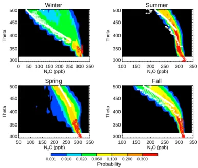
is a source of air for the LMS, thus its composition is relevant. Low N₂O descends to the LMS in winter and spring, while horizontal poleward transport in summer brings higher (tropospheric) mixing ratios. Figure 3 shows seasonal contoured pdfs of model N2O,

the most probable profile from pdfs of MLS N₂O (white lines), and seasonal mean N₂O profiles from ER-2 and SPURT measurements (white and red points, respectively).

25

The contoured pdfs show the most probable values and the range of model variability found. The most probable values in winter represent the vortex mean, while the large variability comes from profiles outside the vortex. (The spring ER-2 data are omitted

(11)

ACPD

7, 1449–1477, 2007

Full Screen / Esc

Printer-friendly Version Interactive Discussion because they are from a year with an unusually late vortex breakup (Coy et al., 1997).)

The only disagreement with the data is found in summer and fall above 450 K, where the model is up to 15% too high. Although the strength of descent and horizontal mixing cannot be judged independently, the excellent model agreement throughout most of the year at levels as low as 320 K suggests a very good balance of vertical and horizontal

5

transport in the polar lower stratosphere. The SPURT measurements are higher than the model in the LMS in winter, but this could be due to weaker descent in the warm Arctic winters in the years of the SPURT campaign (2002 and 2003). The model Arctic temperatures are near or below the real climatological mean.

Variability is an indicator of the presence or absence of transport processes. In

win-10

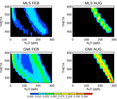
ter, large tracer gradients across the vortex edge coupled with wave-driven vortex wob-ble create high latitude pdfs with large variability. Strong horizontal mixing in spring causes breakdown of the vortex and homogenization of the extratropics. With very weak wave-driving until mid-fall, the well-mixed extratropics produce pdfs with very low variability in the summer months. Figure 4 demonstrates the realistic seasonal

vari-15

ability of high latitude transport and mixing processes in the GMI model. In February, excellent agreement between MLS and the model most probable profiles inside and outside the vortex, and the variability in both regions, shows that the model vortex is well isolated. The model has more points between the two profiles, indicating slightly more mixing across the vortex edge. In summer, the MLS data and the model both

20

show low variability characteristic of a well-mixed atmosphere with little wave-driving. Close agreement with MLS variability is also seen in the months not shown.

Figures 3 and 4 show that the model lower stratosphere provides realistic input for the LMS in all seasons. To examine transport characteristics and composition in the LMS, we look at SPURT N2O in the dynamical coordinate system of equivalent latitude

25

and potential temperature. The use of equivalent latitude, which maps each measure-ment onto latitude according to its potential vorticity, removes variability caused by reversible wave transport [Butchart and Remsberg, 1986; Nash et al., 1996]. H2004 and Hegglin et al. [2006] used this coordinate system to show that the isopleths of CO,

(12)

ACPD

7, 1449–1477, 2007

Full Screen / Esc

Printer-friendly Version Interactive Discussion N₂O, and O₃follow PV contours rather than those of potential temperature in the LMS

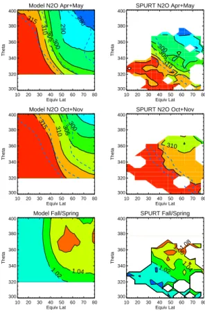
(<360 K) in all seasons. Figure 5 shows the model and SPURT N2O in the spring and

fall; the dashed lines are PV contours (2, 4, and 6 PVU). Note that the PV contours cross isentropes, or equivalently, there are PV gradients on the isentropic surfaces. The PV gradients hinder horizontal transport, allowing time for diabatic cooling in the

5

middleworld to move tracer isopleths downward as they are transported poleward. Be-cause the model N₂O isopleths, like the data, clearly follow the dynamical tropopause and PV contours, this suggests the model has a reasonable balance between horizon-tal transport and diabatic cooling in the LMS. In all seasons except winter, model N2O

mixing ratios are always within 2% of SPURT values. As noted before, SPURT values

10

are probably high in winter due to weak descent in the observation years.

Figure 5 also contrasts the composition differences between spring and fall. In spring, downward advection by the Brewer-Dobson circulation is at a maximum, re-sulting in relatively low N₂O, and in fall, the downward circulation is weak and the influ-ence of horizontal transport from the tropics is greatest (higher N2O), consistent with

15

the Hegglin et al. (2006) analysis of transport using SPURT N2O. The bottom panels

show the ratio of fall to spring mixing ratios. The ratio is proportional to the seasonally changing tropospheric fraction of air in the LMS and is very well represented by the model as a function of both height and latitude.

3.2.2 Ozone

20

Ozone is also an excellent lower stratospheric transport tracer. The availability of global MLS O3 measurements down to 215 hPa allows evaluation of the entire LMS and

the tropical UT (the middleworld). Ozone in the middleworld is controlled largely by transport, although O₃production and loss are sensitive to local NO_x. Figure 6 shows the annual cycle of O3 from the tropics to high latitudes, from 350 K–420 K using MLS

25

data (black). Model O3data are overlaid in red. (ER-2 data are not used here because

they are only available as seasonal means.) Overall, the model shows exceptional agreement with the observed annual cycles and their variability. Model ozone in the

(13)

ACPD

7, 1449–1477, 2007

Full Screen / Esc

Printer-friendly Version Interactive Discussion tropics is ∼50 ppb too low at all levels but shows the right seasonal variation, including

the summer maximum seen in the MLS data. The low model O₃ could indicate an insufficient source of O3 from lightning-produced NOx in the tropical UT, or insufficient

exchange with the midlatitudes, a source of higher O3. This discrepancy is so small

that as a percentage it appears insignificant at higher levels (<10%). The model high

5

latitude O3 shows near perfect agreement in all seasons at all levels shown. Model

midlatitude O3looks good in summer and fall but is low in winter. This cannot easily be

explained by horizontal transport problems. If the vortex were too isolated, this would act to reduce the amount of high O3mixed into the midlatitudes; however, Fig. 4 shows

that the vortex is not overly isolated. And tropical O3 is low, indicating, if anything,

10

too little exchange with midlatitudes. This leaves insufficient midlatitude descent as a possible cause for the low O3 in winter. Overall, the agreement between observed

and model O3 in the middleworld and LS shown in Fig. 6 is quite close when put

in the context of the large range of observed mixing ratios here. Because variability and seasonal composition are controlled by transport, the O3 and N2O diagnostics

15

demonstrate credible model transport throughout the year in the extratropical lower stratosphere from 320 K–500 K.

3.3 Stratosphere-troposphere coupling at the extratropical tropopause

3.3.1 CO and O3

CO and O₃have different source regions and hence different correlations in the

tropo-20

sphere and stratosphere. Near the extratropical tropopause, these opposite correla-tions are connected by lines with CO and O3mixing ratios intermediate between their

tropospheric and stratospheric values (Pan et al., 2004; H2004). H2004 assessed the degree of coupling between the stratosphere and troposphere by measuring the thick-ness of the mixed layer near the tropopause. Using the dynamical tropopause (2 PVU)

25

as a reference, they found that this mixed layer began just below the tropopause and extended to ∼25 K above it, and that the thickness of this layer was the same in all

(14)

ACPD

7, 1449–1477, 2007

Full Screen / Esc

Printer-friendly Version Interactive Discussion sons and latitudes in the extratropics. They also found that the thermal tropopause was

usually slightly above the 2 PVU tropopause. On an absolute scale, the 350 K surface was almost always above the mixed layer during the SPURT campaigns at latitudes 50◦_{N or higher. These results are consistent with the tracer studies of Chen(1995),}

who reported that vigorous exchange between the stratosphere and troposphere

oc-5

curred year-round at 330 K and below due to breaking synoptic scale baroclinic dis-turbances. This is in contrast to their “middle” middleworld results (350 K and above), where seasonal mixing across the subtropical jet was found to be enhanced by the monsoon anticyclones in summer and prohibited by large PV gradients in winter.

We diagnose the model’s strat-trop interaction region by the thickness of its mixed

10

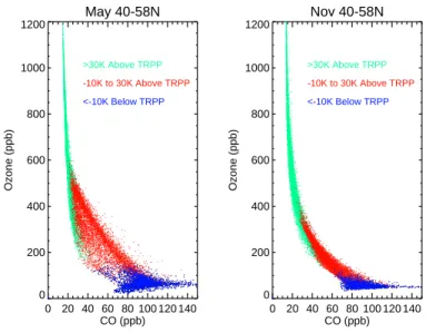
layer and location with respect to the dynamical tropopause. This method was used on aircraft observations by Hoor et al. (2002). Figure 7 shows model CO and O3

where heights with respect to the tropopause are color coded. At >30 K above the tropopause (green), CO is near its minimum (stratospheric) value, while <–10 K below the tropopause (blue), O3 is near its minimum (tropospheric) value. The red points

15

form mixing lines between the two regions and range from –10 K below to 30 K above the tropopause. The mixing lines are broadest in spring due to large variability in the upper tropospheric and lower stratospheric reservoir regions, indicating that different air masses (e.g. vortex and nonvortex) are involved in mixing. The mixing lines are most compact in fall when the reservoir regions are more homogeneous. We find that

20

the thickness of the model mixed layer is nearly constant with latitude and season and the mixed layer extends no more than 30 K above the dynamical tropopause, just as in the SPURT data analysis (H2004). This suggests that the model provides reasonable forcing by synoptic scale disturbances in the UT throughout the year that couple the model’s troposphere with the lowest layers of the stratosphere.

25

3.3.2 CO2

The CO₂seasonal cycle phase and amplitude at the extratropical tropopause not only demonstrate the coupling between troposphere and stratosphere, but can be used to

(15)

ACPD

7, 1449–1477, 2007

Full Screen / Esc

Printer-friendly Version Interactive Discussion diagnose the influence of air arriving via the tropical stratosphere at levels above the

coupling. Figure 8 shows the model CO₂ cycle 40◦_–60◦_{N at several levels above and}

below the 2 PVU tropopause. The observed cycles in the UT and at the tropopause both have a spring maximum and a large amplitude (blue), but above that there are sig-nificant differences in phase and amplitude (Nakazawa et al., 1991; H2004). At +20 K

5

(green) the amplitude is much lower than below and the maximum occurs more than a month later; these features suggest a mixture of influences from above and below, consistent with the mixed region diagnosed by the CO-O₃ scatterplots. At +40 K and above (orange and red), a purely stratospheric cycle appears, with low amplitude and a maximum shifted to late summer. As has been demonstrated by analysis of

obser-10

vations in H2004, B96, and Strahan et al. (1998), this cycle arrives via ascent through the tropical tropopause, followed by meridional poleward transport. The seasonal max-imum that occurs in May in the northern mid-high latitude lower troposphere requires ∼3 months to travel to the midlatitude LS via the tropical tropopause. A key feature of this diagnostic, shown clearly in Fig. 9 of H2004, is the presence of a reversed vertical

15

gradient in late summer, with low CO2 in the UT and high CO2 in the LS (near day

250). In all other seasons CO₂ decreases with height. The timing and magnitude of the model gradient reversal is in good agreement with the H2004 analysis that showed a 2–3 ppm difference between the UT and 40–60 K above the tropopause in August. A model run with convection turned off failed to produce the low CO2 in the UT in

sum-20

mer and the reversed gradient, demonstrating the importance of convection to correctly simulate composition near the tropopause. The GMI model shows a UT amplitude of 5–6 ppm, in excellent agreement with Fig. 9 of H2004.

4 Diagnostics summary and GMI Combo Model Credibility

Table 1 summarizes the suite of transport diagnostics presented in this paper. They

25

have been applied to the GMI GEOS4-GCM Combo CTM to evaluate transport from the tropical upper troposphere to the lower stratosphere, composition of the lowermost

(16)

ACPD

7, 1449–1477, 2007

Full Screen / Esc

Printer-friendly Version Interactive Discussion stratosphere, and coupling between the troposphere and stratosphere. Most

compar-isons with data showed excellent agreement, but a few discrepancies were found in the analysis of tropical transport. Ascent from tropical tropopause to 435 K appeared to be a little too rapid in summer and the CO2cycle amplitude was attenuated too much

as it ascended, suggesting too strong mixing with the midlatitudes. This is consistent

5

with summer polar N2O profiles being too high (too tropospheric). The Brewer-Dobson

circulation in the GEOS4-GCM appears to be too strong at these altitudes in the warm seasons.

The observationally-derived diagnostics indicate two distinct regions within the low-ermost stratosphere. The upper region, ∼350 K–380 K, has seasonally varying

com-10

position, while the lower region, a ∼30 K thick layer above the tropopause, shows uni-form composition (excluding CO2) and thickness year-round. In this lower region, the

bulk of the comparisons demonstrate that the GMI Combo CTM has composition and transport characteristics that mirror the observations. The thickness of the mixed layer separating the troposphere and stratosphere (<350 K) agrees closely year-round with

15

the SPURT data, and the phase and amplitude change of the CO2 cycle across the

tropopause is in agreement with the Nakazawa et al. (1991) and H2004 results. This suggests that the UT wave disturbances involved in creating the mixed layer (Chen, 1995) operate realistically year-round. SPURT data analyses have shown that trans-port of long-lived species (N2O, O3, and CO) follow isopleths of PV rather than

poten-20

tial temperature. Model tracer transport also follows PV isopleths. Downward transport out of the LMS (stratosphere-to-troposphere flux) was not been evaluated here but was been previously estimated for meteorological fields from the same GCM (Olsen et al., 2004). They compared ozone fluxes with empirically derived mass fluxes (Olsen et al., 2003) and found the absolute values and their seasonal variations were reasonable.

25

There is also good agreement in the middle and upper LMS (350–380 K) where there is a clear annual cycle in the composition. The annual cycle arises from the seasonally-varying influence of the stratosphere (strong downward motion in winter) and troposphere (horizontal transport of tropical air via monsoon anticyclones in

(17)

ACPD

7, 1449–1477, 2007

Full Screen / Esc

Printer-friendly Version Interactive Discussion mer). Realistic model transport in this region is supported by O₃seasonal cycles from

the tropics to high latitudes which match extremely well with MLS observations for 2005, and by the ratio of fall/spring N2O, which shows the seasonal influence from the

troposphere and matches the SPURT data very closely. Middleworld composition de-pends on the composition of stratospheric air descending from above, and the close

5

agreement of high latitude N2O profiles with MLS, SPURT, and ER-2 data suggests

realistic input from the overlying lower stratosphere in all seasons.

Model evaluation in the lower stratosphere is essential because a credible lower stratosphere is a prerequisite for a credible middleworld. Realistic transport into and within the lowermost stratosphere depends on Brewer-Dobson circulation in the

mete-10

orological fields used in a CTM. In the analysis of a similar CTM using GEOS4-GCM fields, Strahan and Polansky (2006) found that realistic lower stratospheric transport barriers (e.g., those near the polar vortex and in the subtropics) were essential for ob-taining credible O₃ and CH₄ distributions. Meteorological fields known to have good barriers (e.g., the GEOS4-GCM) still require a CTM horizontal resolution of at least

15

2◦

×2.5◦in order to correctly produce the barriers in the CTM. Observationally-derived transport diagnostics used in Strahan and Polansky (2006) as well as several previous GMI studies are recommended for evaluation of stratospheric transport (Douglass et al., 1999; Strahan and Douglass, 2004).

The realistic seasonal cycle of transport into and within the GMI lowermost

strato-20

sphere shown here demonstrates the utility of this model for studies of the influence of tropospheric composition on the lower stratosphere. The model shows a reason-able transport time from the surface to the tropical upper troposphere, and in summer and fall the model transports tropical UT air into the lowermost stratosphere (∼350 K– 380 K). This demonstrates the feasibility of using this model to study the effects of

tropo-25

spheric pollutants with a life time of even a few months on the composition, chemistry, and radiative properties of the LMS. The seasonally varying O3 composition matches

extremely well with observations, which supports the use of this model in studies involv-ing perturbations to O₃. This model can be credibly used to study problems such as the

(18)

ACPD

7, 1449–1477, 2007

Full Screen / Esc

Printer-friendly Version Interactive Discussion impact of large emissions from fires on the stratosphere and the impact of short-lived

halogenated species on ozone loss in the lowermost stratosphere.

Acknowledgements. This work is supported by the NASA Model Analysis and Prediction

Pro-gram. We thank J. Rodriguez, Project Scientist of the Global Modeling Initiative for scientific support and E. Nielsen for producing the GEOS-4-GCM meteorological fields. We also thank

5

N. Livesey and L. Froidevaux for use of the MLS version 1.5 ozone data.

References

Bey, I., Jacob, D. J.,Yantosca, R. M., et al.: Global modeling of tropospheric chemistry with assimilated meteorology: Model description and evaluation, J. Geophys. Res., 106, 23 073– 23 095, 2001.

10

Bian, H. and Prather, M.J.: Fast-J2: Accurate simulation of stratospheric photolysis in global chemical models, J. Atmos. Chem., 41, 281–296, 2002.

Bloom, S. C., da Silva, A. M., Dee, D. P., et al.: The Goddard Earth Observation System Data Assimilation System, GEOS DAS Version 4.0.3: Documentation and Validation, NASA TM-2005-104606 V26, 2005.

15

Boering, K. A., Wofsy, S. C., Daube, B. C., Schneider, J. R., Loewenstein, M., Podolske, J. R., and Conway,T. J.: Stratospheric mean ages and transport rates from observations of CO₂ and N₂O, Science, 274, 1340–1343, 1996.

Butchart N. and Remsberg, E. E.: The area of the stratospheric polar vortex as a diagnostic of tracer transport on an isentropic surface, J. Atmos. Sci., 43, 1319–1339, 1986.

20

Chen, P.: Isentropic cross-tropopause mass exchange in the extratropics, J. Geophys. Res., 100, 16 661–16 674, 1995.

Conway, T. J., Tans, P. P., Waterman, L. S., and Thoning, K. W.: Evidence for interannual variability of the carbon-cycle from the National Oceanic and Atmospheric Administration Climate Monitoring and Diagnostics Laboratory Global Air Sampling Network, J. Geophys.

25

Res., 99, 22 831–22 855, 1994.

Coy, L., Nash, E. R., and Newman, P. A.: Meteorology of the polar vortex: Spring 1997, Geo-phys. Res. Lett., 24, 2693–2696, 1997.

Douglass, A. R., Prather, M. J., Hall, T. M., Strahan, S. E., Rasch, P. J., Sparling, L. C., Coy,

(19)

ACPD

7, 1449–1477, 2007

Full Screen / Esc

L., and Rodriguez, J. M.: Choosing meteorological input for the global modeling initiative assessment of high-speed aircraft, J. Geophys. Res., 104, 27 545–27 564, 1999.

Douglass, A. R., Stolarski, R. S., Strahan, S. E., and Connell, P. S.: Radicals and reservoirs in the GMI chemistry and transport model: Comparison to measurements, J. Geophys. Res., D16303, doi:10.1029/2004JD004632, 2004.

5

Dunkerton, T. J.: Evidence of meridional motion in the summer lower stratosphere adjacent to monsoon regions, J. Geophys. Res., 100, 16 675–16 688, 1995.

Engel, A., Boenisch, H., Brunner, D., et al.: Highly resolved observations of trace gases in the lowermost stratosphere and upper troposphere from the SPURT project: an overview, Atmos. Chem. Phys., 6, 283–301, 2006,

10

http://www.atmos-chem-phys.net/6/283/2006/.

Hegglin, M. I., Brunner, D., Peter, T., et al.: Measurements of NO, NOy, N2O, and O3

dur-ing SPURT: implications for transport and chemistry in the lowermost stratosphere, Atmos. Chem. Phys., 6, 1331–1350, 2006,

15

Holton, J. R., Haynes, P. H., McIntyre, M. E., Douglass, A. R., Rood, R. B., and Pfister, L.: Stratosphere-troposphere exchange, Rev. Geophys., 33, 403–439, 1995.

Hoor, P., Fischer, H., Lange, L., and Lelieveld, J.: Seasonal variations of a mixing layer in the lowermost stratosphere as identified by the CO-O₃correlation from in situ measurements, J. Geophys. Res., 107, D4044, doi:10.1029/2000JD000289, 2002.

20

Hoor, P., Gurk, C., Brunner, D., Hegglin, M. I., Wernli, H., and Fischer, H.: Seasonality and extent of extratropical TST derived from in-situ CO measurements during SPURT, Atmos. Chem. Phys., 4, 1427–1442, 2004,

Hoskins, B. J.: Toward a PV-theta view of the general circulation, Tellus, Ser. A, 43, 27–35,

25

1991.

Kinnison, D. E., Connell, P. S., Rodriguez, J. M., et al.: The Global Modeling Initiative Assess-ment Model: Application to High-Speed Civil Transport Perturbation, J. Geophys. Res., 106, 1693–1712, 2001.

Ko, M. K. W., Sze, N. D., Scott, C.J., and Weisenstein, D. K.: On the relation between

strato-30

spheric chlorine/bromine loading and short-lived tropospheric source gases, J. Geophys. Res., 102, 25 507–25 517, 1997.

Lin, S.-J.: A vertically Lagrangian finite-volume dynamical core for global models, Mon Wea.

(20)

ACPD

7, 1449–1477, 2007

Full Screen / Esc

Rev., 132, 2293–2307, 2004.

Lin, S.-J., and Rood, R. B.: Multidimensional flux-form semi-Lagrangian transport schemes, Mon. Wea. Rev., 124, 2046–2070, 1996.

Livesey, N., Read, W. G., Filipiak, M. J, et al.: Earth Observing System (EOS) Microwave Limb Sounder (MLS) Version 1.5 Level 2 data quality and description document, JPL D-32381,

5

2005.

Nakazawa, T., Miyashita, K., Aoki, S., and Tanaka, M.: Temporal and spatial variations of upper tropospheric and lower stratospheric carbon dioxide, Tellus, Ser. B, 43, 106–117, 1991. Nash, E. R., Newman, P. A., Rosenfield, J. E., and Schoeberl, M. R.: An objective determination

of the polar vortex using Ertel’s potential vorticity, J. Geophys. Res., 101, 9471–9478, 1996.

10

Olsen, M. A., Douglass, A. R., and Schoeberl, M. R.: Estimating downward cross-tropopause ozone flux using column ozone and potential vorticity, J. Geophys. Res., 107, D4636, doi:10.1029/2001JD002041, 2002.

Olsen, M. A., Douglass, A. R., and Schoeberl, M. R.: A comparison of Northern and Southern Hemisphere cross-tropopause ozone flux, Geophys. Res. Lett, 30, 1412,

15

doi:10.1029/2002GL016538, 2003.

Pan, L. L., Randel, W. J., Gary, B. L., Mahoney, M. J., and Hintsa, E. J.: Definitions and sharpness of the extratropical tropopause: A trace gas perspective, J. Geophys. Res., 109, D23103, doi:10.1029/2004JD004982, 2004.

Ray, E. A., Moore, F. L., Elkins, J. W., Dutton, G. S., Fahey, D. W., Vomel, H., Oltmans, S. J., and

20

Rosenlof, K. H.: Transport into the Northern Hemisphere lowermost stratosphere revealed by in situ tracer measurements, J. Geophys. Res., 104, 26 565–26 580, 1999.

Rotman, D. A., Tannahill, J. R., Kinnison, D. E., et al.: Global Modeling Initiative assessment model: Model description, integration, and testing of the transport shell, J. Geophys. Res., 106, 1669–1691, 2001.

25

Salawitch, R. S., Weisenstein, D. K., Kovalenko, L. J., Sioris, C. E., Wennberg, P. O., Chance, K., Ko, M. K. W., and McLinden, C.A.: Sensitivity of ozone to bromine in the lower strato-sphere, Geophys. Res. Lett., 32, L05811, doi:10.1029/2004GL021504, 2005.

Schoeberl, M. R., Duncan, B. N., Douglass, A. R., Waters, J., Livesey, N., Read, W., and Filipiak, M.: The carbon monoxide tape recorder, Geophys. Res. Lett., 33, L12811,

30

doi:10.1029/2006GL026178, 2006.

Strahan, S. E., Douglass, A. R., Nielsen, J. E., and Boering, K. A.: The CO₂seasonal cycle as a tracer of transport, J. Geophys. Res., 103, 13 729–13 742, 1998.

(21)

ACPD

7, 1449–1477, 2007

Full Screen / Esc

Strahan, S. E., Loewenstein, M., and Podolske, J. R.: Climatology and small-scale structure of lower stratospheric N₂O based on in situ observations, J. Geophys. Res., 104, 2195–2208, 1999.

Strahan, S.E.: Climatologies of lower stratospheric NO_y and O₃ and correlations with N₂O based on in situ observations, J. Geophys. Res., 104, 30 463–30 480, 1999.

5

Strahan, S. E. and Polansky, B. C.: Meteorological implementation issues in chemistry and transport models, Atmos. Chem. Phys., 6, 2895–2910, 2006,

Waters, J., Froidevaux, L., Harwood, R. S., et al.: The Earth Observing System Microwave Limb Sounder (EOS MLS) on the Aura satellite, IEEE Trans. Geosci. Remote Sensing, 44,

10

1075–1092, 2006.

Wild, O., Zhu, X., and Prather, M.: Fast-J: Accurate simulation of in- and below-cloud photolysis in tropospheric chemical models, J. Atmos. Chem., 37, 245–282, 2000.

World Meteorological Organization (WMO), Scientific assessment of ozone depletion: 2002, WMO 47, Geneva, Switzerland, 2002.

15

(22)

ACPD

7, 1449–1477, 2007

Full Screen / Esc

Table 1. Transport diagnostics for the upper troposphere and lowermost stratosphere.

Region Feature Reference Surface to UT CO₂ cycle phase and amplitude at

tropical stratospheric entry (∼380 K)

Boering et al. (1996) Troposphere to

Stratosphere (vertical)

CO₂ cycle phase and amplitude at 435 K in tropics

Boering et al. (1996)

Troposphere to Stratosphere (isentropic)

CO₂ cycle phase and amplitude at ∼380 K, 40◦N

Boering et al. (1996)

O₃ seasonal cycle amplitude and variability, tropics to high latitudes, 350 K–420 K This study. Composition and Coupling in the LMS, Transport within the LMS N₂O Seasonal Profiles, 70◦_–88◦_N, 320–500 K This study. Ratio of Fall/Spring N₂O, 320–380 K (change in tropospheric fraction of LMS air)

This study.

CO, O₃, and/or N₂O isopleths follow-ing the tropopause

Hoor et al. (2004) Consistent thickness of mixed layer

at the extratropical tropopause

Hoor et al. (2004) Change in CO₂cycle amplitude from

the UT to the LS

Nakazawa et al. (1991), Hoor et al. (2004)

(23)

ACPD

7, 1449–1477, 2007

Full Screen / Esc

Printer-friendly Version Interactive Discussion -50 0 50 LATITUDE 1000 100 PRESSURE January 190 210 210 210 230 230 230 250 250 270 270 290 290 290 320 320 350 350 380 380 440 440 500 500 560 560 620

1

2

3

4 LMS

UT

LS

Fig. 1. Schematic diagram of the lowermost stratosphere derived from zonal monthly mean

GEOS-4 meteorological analyses from January, 2005. Temperature contours are black (dashed), potential temperature contours are blue (solid), and the lowermost stratosphere, de-fined by the 380 K potential temperature surface and the 2 PVU surface, is outlined in red. Transport between the numbered regions is discussed in the text.

(24)

ACPD

7, 1449–1477, 2007

Full Screen / Esc

Surface to Tropopause

0 200 400 600

Days from Jan 1 350 352 354 356 358 Detrended CO 2 (ppm)

Mauna Loa + Samoa (Surface Avg) Strat Entry (380K) 2-Month Lag A Tropopause to 435K 0 200 400 600

Days from Jan 1 351 352 353 354 355 356 357 Detrended CO 2 (ppm) Strat Entry (380K) 435 K 2.5-Month Lag B Tropics to Midlatitudes (390K) 0 200 400 600

Days from Jan 1 353 354 355 356 357 358 359 CO 2 (ppm) Strat Entry 36-40N C

Fig. 2. CO₂ seasonal cycles from two years of the GMI Combo CTM. (a) The black line is the average of Mauna Loa and Samoa boundary conditions (derived from the NOAA Global Monitoring Division Flask Sampling Network), the dashed blue line is that cycle lagged by 2 months, and the red line is the model tropical 380 K cycle, considered to be the stratospheric boundary condition for CO₂. (b) The stratospheric boundary condition at 380 K (red) and the tropical cycle at 435K (solid blue); there is a 2.5 month lag between them. The dashed blue line approximates how the model cycle would look if attenuation and lag followed the aircraft results from B96. (c) The stratospheric boundary condition at 380 K (red) and the CO₂cycle in the midlatitudes, 380–400 K, having N₂O in the range of 305–310 ppb.

(25)

ACPD

7, 1449–1477, 2007

Full Screen / Esc

Printer-friendly Version Interactive Discussion Winter 0 50 100 150 200 250 300 350 N2O (ppb) 300 350 400 450 500 Theta Spring 50 100 150 200 250 300 350 N2O (ppb) 300 350 400 450 500 Theta Summer 100 150 200 250 300 350 N2O (ppb) 300 350 400 450 500 Theta Fall 100 150 200 250 300 350 N2O (ppb) 300 350 400 450 500 Theta 0.001 0.010 0.020 0.060 0.100 0.200 0.300 Probability

Fig. 3. Comparison of GMI N₂O profiles (70–88◦_{N) in four seasons with MLS, SPURT, and}

ER-2 data. Contoured pdfs are averages over the same seasonal sampling periods of the SPURT data (all months of the year sampled except March, June, September, and December). Yellows and reds indicate sharply peaked distributions. MLS data are shown as most probable seasonal values (solid white line). ER-2 data are seasonal means (white points) and SPURT data are seasonal averages (red points).

(26)

ACPD

7, 1449–1477, 2007

Full Screen / Esc

Printer-friendly Version Interactive Discussion MLS FEB 0 100 200 300 N2O (ppb) 450 500 550 600 THETA GMI FEB 0 100 200 300 N2O (ppb) 450 500 550 600 THETA MLS AUG 0 100 200 300 N2O (ppb) 450 500 550 600 THETA GMI AUG 0 100 200 300 N2O (ppb) 450 500 550 600 THETA 0.005 0.010 0.025 0.050 0.075 0.100 0.150 0.200 Probability

Fig. 4. Comparison of GMI and MLS N₂O profile variability (66◦_–82◦_{N). MLS data is shown for}

2005 and 2006. GMI variability is averaged over 2 consecutive model years.

(27)

ACPD

7, 1449–1477, 2007

Full Screen / Esc

Model N2O Apr+May

10 20 30 40 50 60 70 80 Equiv Lat 300 320 340 360 380 400 Theta 280 290 300 305 310 315

SPURT N2O Apr+May

10 20 30 40 50 60 70 80 Equiv Lat 300 320 340 360 380 400 Theta 300 305 310

Model N2O Oct+Nov

10 20 30 40 50 60 70 80 Equiv Lat 300 320 340 360 380 400 Theta 300 305 310 315

SPURT N2O Oct+Nov

10 20 30 40 50 60 70 80 Equiv Lat 300 320 340 360 380 400 Theta 310 Model Fall/Spring 10 20 30 40 50 60 70 80 Equiv Lat 300 320 340 360 380 400 Theta 1.02 _1.04 SPURT Fall/Spring 10 20 30 40 50 60 70 80 Equiv Lat 300 320 340 360 380 400 Theta 1.02 1.04 1.061.08

Fig. 5. N₂O from GMI and SPURT in spring and fall in the dynamical coordinate of potential temperature and equivalent latitude. Potential vorticity contours (2, 4, and 6 PVU) are overlaid with dashed blue lines. Bottom panels show the fall/spring ratio.

(28)

ACPD

7, 1449–1477, 2007

Full Screen / Esc

Printer-friendly Version Interactive Discussion 420K 6-20N 0 100 200 300 DAYS of 2005 0 200 400 600 800 O3 420K 36-50N 0 100 200 300 DAYS of 2005 0 200 400 600 800 1000 1200 1400 O3 420K 60-80N 0 100 200 300 DAYS of 2005 0 500 1000 1500 2000 2500 3000 O3 380K 6-20N 0 100 200 300 DAYS of 2005 0 100 200 300 400 O3 380K 36-50N 0 100 200 300 DAYS of 2005 0 200 400 600 800 1000 O3 380K 60-80N 0 100 200 300 DAYS of 2005 0 200 400 600 800 1000 1200 1400 O3 350K 6-20N 0 100 200 300 DAYS of 2005 0 50 100 150 200 250 300 O3 350K 36-50N 0 100 200 300 DAYS of 2005 0 200 400 600 800 O3 350K 60-80N 0 100 200 300 DAYS of 2005 0 200 400 600 800 1000 O3

Fig. 6. Comparison of GMI (red) and MLS (black) O₃seasonal cycles for three latitude bands and 3 levels in the UT/LS.

(29)

ACPD

7, 1449–1477, 2007

Full Screen / Esc

Printer-friendly Version Interactive Discussion May 40-58N 0 20 40 60 80 100 120 140 CO (ppb) 0 200 400 600 800 1000 1200 Ozone (ppb) >30K Above TRPP -10K to 30K Above TRPP <-10K Below TRPP Nov 40-58N 0 20 40 60 80 100 120 140 CO (ppb) 0 200 400 600 800 1000 1200 Ozone (ppb) >30K Above TRPP -10K to 30K Above TRPP <-10K Below TRPP

Fig. 7. Scatterplot of GMI CO and O₃in the UT/LMS, spring and fall. Points are color-coded by their location with respect to the dynamical tropopause (2 PVU). Blue points are more than 10 K below the tropopause. Green points are more than 30 K above the tropopause. Red points, which are just below and up to 30 K above the tropopause, represent the mixed region near the tropopause.

(30)

ACPD

7, 1449–1477, 2007

Full Screen / Esc

Printer-friendly Version Interactive Discussion Model CO2, 40-60N 0 100 200 300 Days 352 354 356 358 360 CO 2 (ppb) Upper Trop Tropopause +20K +40K +60K

Fig. 8. GMI CO₂ cycles just below, at, and above the midlatitude tropopause. The trend in CO₂ has been removed to clarify the differences in cycle phase and amplitude across the tropopause.