HAL Id: hal-02470609
https://hal.uca.fr/hal-02470609
Submitted on 7 Feb 2020
HAL is a multi-disciplinary open access
archive for the deposit and dissemination of
sci-entific research documents, whether they are
pub-lished or not. The documents may come from
L’archive ouverte pluridisciplinaire HAL, est
destinée au dépôt et à la diffusion de documents
scientifiques de niveau recherche, publiés ou non,
émanant des établissements d’enseignement et de
Technical Report : 3D mesh Segmentation Application
to glasses
Coralie Bernay-Angeletti, Jean-Marie Favreau
To cite this version:
Coralie Bernay-Angeletti, Jean-Marie Favreau. Technical Report : 3D mesh Segmentation Application
to glasses. [Technical Report] LIMOS (UMR CNRS 6158), université Clermont Auvergne, France.
2017. �hal-02470609�
Technical Report : 3D mesh Segmentation
Application to glasses
C. Bernay-Angeletti, J-M Favreau
LIMOS UMR 6158 UBP/ CNRS,
Campus des Cézeaux
63177 AUBIERE Cedex, FRANCE
October 16, 2017
Abstract
Object segmentation in meaningfull parts is an important research topic as these have become a part of many mesh and object manipula-tion algorithms in computer graphics, geometric modelling and computer aided design. In particular, tasks that were before realized by experts are more and more assumed by people without particular formation in geometric or computer graphic problems. So there is a need to have some ergonomic tools that have expert know-how while user keep control on specific constraints to its particular application. Here, we present how for segmentation purpose we model expert know-how and two algorithms that can be used to make segmentation task. One is generic and the other is specialized for glasses segmentations.
1
Introduction
In reason of 3D printers democratisation and easy access to 3D scanners, there is more and more 3D meshes available on internet. So use of 3D mesh becomes commonplace, increasing needs in automatic processings and in interfaces for
computer-aided manipulations. In particular, tasks that were before realized by experts are more and more assumed by people without particular formation in geometric or computer graphic problems. So there is a need to have some ergonomic tools that have expert know-how while user keep control on specific constraints to its particular application. Mesh segmentation has become a key point in many computer graphics tasks and applications and also in geometric modelling. Segmentation can help for parametrization, mesh editing or anima-tion and many other tasks [4, 5]. So segmentaanima-tion is a crucial point when we want to offer tools for automatic processing.
Mesh segmentation partitions the surface into a set of clusters under some criteria often depending of the final application. Comparative survey on seg-mentation technics [1, 16, 24] classify them in two categories: geometric segmen-tation and semantic segmensegmen-tation. We are only interesting in the second one: our aim is to extract meaningful parts (having experts knowledge about what that mean) of an object in reasonable time, as it will ba a pretreatment in a more complete application. Different parts should be well identify because different treatment will be allowed depending on their nature. Automatically identify meaningful parts of a 3D mesh is challenging. A common practice is to build some specific features by extracting some geometric or volumetric properties like approximate convexity anlysis [8], concavity-aware field [2], spectral clus-tering [12], K-means [18], core-extraction [9], graph-cuts and randomized cuts [6], randomwalk [11] and then use it for segmentation purpose. Part boundaries or frontiers are faces which have at least one neighbor with a different label (that is which belongs to another part than theirs). Inducing part boundaries along negative curvature minima is often used even for semantic segmentation because they often offer natural separation between parts like legs and torso. Volumetric considerations can also be used and are more related to skeletal shape representation like shape diameter function [17].
Rathers than trying to segment a single object some recent researches are done on co-segmentation [7, 13, 19, 20, 25]: the aim is to segment in the same time a family of objects (for example different glasses) because more semantic knowledge can be extracted by simultaneously analyzing a set of shapes instead of a single shape. But their final objective is shlightly different of ours as they only guarantee consistent segmentation over the set whereas we want to use expert knowledge about what is for a given problem a good segmentation. In-deed, often saying what is meaningful parts or good segmentation is not a so easy task. Good exemples of that can be found in [5] where users are asked to seg-ment different objects. We can see that different persons segseg-ments same object differently (see figure 1). Why one should be consider better than another?
That why, we consider that we have at least an exemple of good segmentation in the sense that it has be done by an expert and so it can be considered well-suited for its specific problem. In consequence, here, expert knowledge will be represent by at least one shape and its good segmentation and our aim will be : given another shape of the same family, how can we segment it so that extracted meaningful parts are coherent with example shape.
Figure 1: An exemple of segmentations of the same objet, here glasses, from different persons. Segmentations can be found in http://segeval.cs. princeton.edu/, details of segmentations process are described in [5].
2
Strategy
2.1
Context
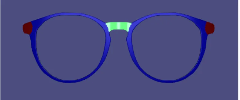
Our project implies at the same time a local company Polymagine and a research laboratory LIMOS. Company needs directed areas of research so that proposed solutions can be used in industry in the long run. In particular, we will take care about time computations and will try to have few constraints for meshes (we will not fixe number of vertices or faces for example). Polymagine is specialized in personnalisation of objects. Polymagine is interesting in segmentation as a pre-processus before personnalisation step : deformation and transformation cannot be apply in the same way on all the object. They represent the expert knowledge and provide us some segmentations examples for glasses (see figure 2). So, glasses are for us composed of tenon (in red) on which will come to hang on the legs of glasses, circles (in blue) which hold glasses and finally bridge (in green) which connects both circles. We assume that we have at least one labelled example of glasses but not a lot.
Figure 2: Good segmentation of glasses. Tenons are in red, circles in blue and bridge in green.
2.2
Learning with (deep) neural network
Deep learning is widely used in image segmentation process. AlexNet [10] is one of the more known deep neural network. It is one of the pioneer in deep CNN. Visual Geometry Group (VGG) [21] and GoogLeNet [23] are two others very well known deep neural network for image segmentation. They give good results. Even if CNN (Convolutionnal Neural Network) cannot be used for mesh segmentation because of the complexity of 3D geometry (a vertice don’t have all the time the same number of neigboor whereas in an image the number of pixels surrounded one pixel is fixed), it seems to us that neural network can be interesting in our case, as we want to transfer knowledge from given examples to new examples of same family.
2.3
Features
When using neural network, what are entries is one of first question to answer. As previously stated, vertices (or faces) of meshes are not good candidates because they can vary in number and it is difficult to order them : what can be consider as first vertice and how we traversed the others ? So we make the choice to work as in more classical mesh segmentation technics with particular features.
We find that the work of [25] is interesting. Their aim is not exactly the same as they want to make co-segmentation and so do not have a model to respect in segmentation. They compute presegmentations (rough segmentations) of a family of meshes using K-means in space of eigenfunctions of Laplace-Beltrami [3, 14]. Then they use these presegmentation and properties of Laplace-Beltrami operator to compute Functional Maps [15] and to make correspondance between parts of differents objects. Then, they are able to make segmentation of their family of meshes. Results on differents family of shapes are impressive.
We make some preliminary tests using the code for Functional Maps provided on http://www.lix.polytechnique.fr/~maks/fmaps_course/publications. html. To use this code, we need to have a pre-segmentation of meshes, that is a segmentation in some coarse regions and we need meshes with the same number of vertices. This two conditions are for us only for tests, because we want to be able to treat meshes from our industrial partner that will not respond to this criteria (meshes tend to have the same order of vertices but not exactly the same number).
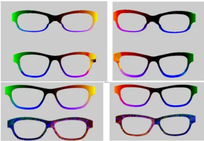
On figure 3, tree pre-segmentations are showns. On figure 4, results of Func-tionals Maps given the previous pre-segmentation are shown. Colors indicates similar regions. On the first sub image, the second glasses (the upper one) has been created by deformation of the first glasses (on bottom). Matching between the two shapes is not perfect in particular near the bridge but it seem to be promising. At contrary, on second subimage, the two shapes have independant meshes and matching is really bad.
Functional Maps not seem to be well-suited for our problematic were meshes are not near isometric deformation one from another. Nevertheless, we keep
Figure 3: Pre-segmentations for tree differents glasses : glasses a), glasses b) and glasses c).
Figure 4: Functional Maps used on our glasses. First column shows front of glasses and second columns the back. Fisrt rows is between glasses b) and a). Second rows is between glasses a) and c). Same colors should indicate correspondant regions.
Figure 5: On first row : 1st, 2nd eigenfunctions of Laplace-Betrami. On second rpw : 3rd and 4th eigenfunctions of Laplace-Beltrami.
being interesting in the Beltrami Operator as features. Indeed Laplace-Beltrami is a local descriptor where different feature information are represented by different feature functions. Since eigenfunctions of Laplace-Beltrami are or-der from low-frequencies to high-frequencies. Yet low-frequencies contain more information than high-frequencies functions. So a few of Laplace-Beltrami eigen-functions can be used as features descriptors. Advantage of Laplace-Beltrami eigenfunction are that they are independant from shape spacial localisation and that it describe well shape geometry. In figure 5, the 4 first eigenfunctions of Laplace-Beltrami are shown.
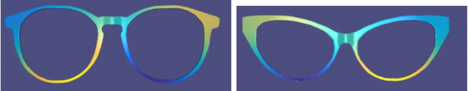
On experiments, there can be some problems of flips in Laplace-Beltrami eigenfunctions : sometimes sign of similar regions are inverted. An exemple is given on figure 6. On the first glasses, high value (in yellow) are on bottom-left circle and upper-right circle whereas on the second glasses it is on bottom-right circle and upper-left circle. To overcome this problem of flip signs, we simply consider the absolute value of the Laplace-Beltrami eigenfunctions. We will also normalize eigenfunction to be between 0 and 1 :
φ∗i = |φi| − minj|φi(xj)| maxj|φi(xj)| − minj|φi(xj)|
(1) where :
• φ∗
i : is the ith feature used. It is the ith eigenfunction of Laplace-Beltrami
in absolute value and normalized.
• φi is the ith eigenfunction of Laplace-Beltrami.
• xj is a vertice of the mesh
• | − | represents the absolute value.
In fact, we are more interested in having one label per face than having one label per vertice so we convert this vertice features in face features. To make
Figure 6: the 4rd eigenfunction of Laplace-Beltrami for two differents glasses. We can observed change in sign.
that, for a face f , we consider the 3 vertices which compose it (as we work on triangulated mesh) and we say that the feature face value is the mean of the 3 features vertices. φ∗i(fk) = 1 3 3 X j=1 φ∗i(vkj) (2) where : • φ∗
i(fk) is feature vector computed for face fk and we will refer to it by
absolute-normalized eigenfunctions of Laplace-Beltrami for face fk.
• φ∗
i(vkj) is the absolute-normalized eigenfunctions of Laplace-Beltrami for
a vertice vkj that is one of the 3 vertice of the face fk.
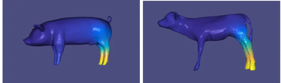
By default, when we will refer to this face feature, we will named these absolute normalized eigenfunctions of Laplace-Beltrami (and we will ommitted for face). Another problem with the Laplace-Beltrami eigenfunction is an ordering problem : even if all regions can be well characterized by these functions, some-times it is not the same function that represent correspondant regions. Whereas sign flip can be easily removed by taking the absolute value of eigenfunction, there is no solution for this ordering problem. Or order has big importance when we want to use neural network. A node should always represent the same com-ponent. Or if there is change in order, it will not be possible. An exemple of this problem is illustrate in figure 7. For illustration purpose, we have change ob-jects and show images on animals but problem is the same on glasses. Here, leg regions are represented one time by the 3rd eigenfunction of Laplace-Beltrami and on other on the 4th eigenfunction.
2.4
Construction of our neural network
To construct our neural network, we have to take into account to the previous remarks and to industrial time constraint : we want that segmentation process can be used in some application so that should not take to much time. As we are only developping some prototype, a time of few minutes (5 minutes should be the maximum and if possible less than one minute) is the goal fixed by Polymagine, considering this computation time could be improved if technics give good results.
Figure 7: eigenfunction of Laplace-Beltrami that highlights the back legs of the two animals. For the pig, it is the 4th eigenfunction whereas for the veal it is the 3rd.
Another important constraint is that we want to treat any mesh given so number of vertices or faces cannot be fixed and our neural network must be able to work with. Often, when size of example if not fixed, RNN (Recurrant Neural Network) are used, in particular for text recognition. But, we think it was not suitable for us, as a sequence has natural order : place of words in sentence (or place of letters in words) are important : verb is after subject and so on. In meshes, ordering is difficult, there is no natural beginning or end of meshes. That why, we decide to take in entry only feature for one face. Doing this, all size of meshes can be treated, if a mesh has n faces, we simply need to use n times our neural network only changing entries. As we give only one face after another, we cannot ensure topological consistence from neural network but we think that absolute-normalized eigenfunctions of Laplace-Beltrami contain enough information about face neighbourhood to ensure coherent segmentation. The main problem that remains is an ordering problem. As discussed previ-ously, absolute-normalized eigenfunctions of Laplace-Beltrami can have different order in different meshes. So we cannot make training on some glasses and then used trained neural network on new glasses. Our main idea, that is really differ-ent from usual use of neural network, was that we do not need to learn on a lot of faces and that only few faces can be used to make training. Idea is to have for one particular mesh few labelled faces per class that are well positionned and to transfert this face (like some initial source seeds) to another glasses. Once, we have for new glasses, some labelled faces we can make training with our features faces for new glasses on this few labelled faces (on new glasses) and then we only need to used the trained neural network on all faces of new glasses. As training is on features from new glasses, there is no problem of order (in one mesh, order is always consistent).
With this idea, we choose to construct a neural network with only one hidden layer considering that as we want to train with few data, we will not have enough data to learn a lot of weighs in a lot of hidden layers. The other good point, in having a small neural network is that training step will be fast (as testing step). We have a fully connected neural network with 50 entries (the 50 first absolute normalized eigenfunctions of Laplace-Beltrami) , 3 outputs (one per class) and
250 nodes on hidden layer. Activation functions from entries to hidden layer are sigmoïds and activation functions from hidden layer to output are softmax functions.
3
Method 1 : Seed Transfert
In this section, we will present in more details our method using the previous idea.
3.1
First Tests
During the analysis phase, we made hypothesis and thus first step is to verify them. We begin by trying to learn segmentation on mesh when we manually select the seeds. Good selection of seeds imply :
• every class should have the same number of seeds. Seeds must be balanced in number.
• in every class, seeds must be spacially distributed. Seeds should be as far away from other seeds of same class as possible.
• in every class, some seeds must be near boundaries : if we segment every face in mesh, some seed must be near a face of different label (this face is not necessary a seed even for the other class).
We compute for all face of meshes, absolute-noramlized eigenfunctions of Laplace-Beltrami. We use 10 seeds per class (for a total of 30 seeds) to train our neural network and after we use the trained neural network for testing segmentation on all faces. Figure 8 shows results for one glasses. Segmentation is coherent with what we want and so it seems that our idea can work.
3.2
Seeds Transfer
To have an automatic process, we want to have an algorithm that is able to tranfer seeds from source mesh (we know source seeds labels) to target mesh.
We want to label the same number of faces in target mesh than in source mesh. Labelled faces in taget mesh will become seeds for target mesh.
3.2.1 Distance Transfer
Firstly, we consider we have aligned glasses. Under this hypothesis, tranferring seeds can be seen as a research of k-nearest neighbour where k = 1, tree is constructed using target mesh face (the center of face is taken as 3D point) , query points are center of seeds in source mesh. The target face that is selected become a seed for target mesh with same label as source seed.
3.2.2 Distance Transfer + eigenfunctions
As glasses have not all exactly the same shape, distance transfer can be improved by taking into account more topological information. For every seeds in source mesh, we will find the k-nearest neighbour where k = 250. This ensure a spacial coherence. But after to select the final target face, we compute distance between the 3 first eigenfunctions of Laplace-Beltrami, the face with the lower distance is kept as target seed. The idea is that eigenfunction of Laplace-Beltrami will probably be more similar on place that have similar function in glasses.
Results of the two transfer can be seen in 5.1.
4
Method 2 : Training
We are also interesting to see if we can use our neural network to make some more usual training as the context change a little bit and more labelled glasses are available. Like we previously discuss, using absolute-normalized eigenfunction of Laplace-Beltrami is not suitable for this purpose so we have to change our features.
We choose to use HKS (Heat Kernel Signature) [22]. As previously, we will take it in absolute value, normalize it and compute a mean to have features for face. So we will named it absolute-normalized HKS. We believe theses features will be less sensitive to the ordering problem. We choose to take 50 features.
We used k glasses to make training. On every glasses we randomly select n faces for every class. So we have kn examples in training set. We train our neural network (the one described in 2.4) only one time with these examples (training can be long). After, we compute for every new glasses, its absolute-normalized HKS features and use the trained neural network on every face by changing entries. Results are shown in 5.2.
5
Results
In this section, we will present some results obtained from the two methods. To implement our algorithmes, we use Matlab to compute generealized eigenvectors and values, Tensorflow in Python to construct, train and use neural network and
C++ to compute features on mesh and make file readable by Matlab or Python. For a mesh with near 23914 vertices and 47832 faces, we need to :
• compute mass matrix and cotangent matrix : 1.4 s • compute generalized eigenvectors and eigenvalues : 21.6 s
• select seeds 4.9s using distance only or 7.6 s using distance + eigenfunc-tions
• compute normalized-absolute eigenfunctions of Laplace-Beltrami using pre-vious steps and writing file test : 12s
• train our neural network : 3.4s
• use trained neural network on all faces : 6.5s
5.1
Result for the first method
Conditions : on one glasses, 10 faces (seeds) per class are well selected. Se-lected face are well balanced in every class region and somme of them are near boudaries. All meshes are aligned. As describes in section 3.2, we use two methods for transfert. The first one take into account only euclidean distance between faces, the second one select for each source face, the 100 nearest target faces and among this 100 target faces, the one with the most similar 3 first eigenfunction is chosen.
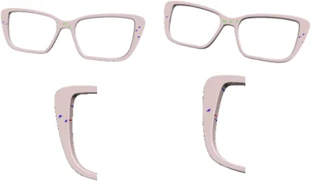
Figure 9 shows one case of mislabelling in transfert in both methods. On the left, it is the distance transfert and on the right it is the distance + eigenfunction transfert.. We can see error in labelling in left tenon, more visible in the second line.
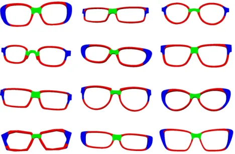
In figure 10, we compare the results on both transfert on 12 glasses. First column reprensents results using transfert with distance only (and after training with seeds and testing) and second column represents results using transfert with distance and eigenfunction (and after training with seeds and testing). Results with distance and eigenfunction give a little bit better results. But two are not perfect segmentation and some glasses are bad segmented. The problem comes from error in labelling as first cause, and position of labelled seeds : they are not as well balanced as in source mesh (they can be less distant or it can lack of seed near boundaries).
Figure 9: Example of transfert labelling. In light grey it is not labelled face, in blue, it is tenon faces, in green bridge faces and in red circle faces. First line show labelled faces on full mesh and second line is a zoom on the left tenon to show error in labelling process. Fisrt column is labelling using transfert with only distance. Second colum is labelling using transfert with distance and eigenfunctions.
Figure 10: First column represents results after transfert with distance only, training and testing. Second columns represent results after transfert with dis-tance and eigenfunction, training and testing.
5.2
Result for the second method
Conditions : we use one glasses as training glasses. We consider we have a good segmentation for all the faces of the mesh. Among this faces, we randomly select 750 in every class, no particular care is done about the repartition of selected faces. Absolute-normalized HKS is computed for each face of all the meshes we want to test. Computing it take 72.3 s. Neural network is the one described in 2.4. Training take 196 s.
In figure 11, the result on the training glasses is shown. Mesh has near 25000 faces. Note that, segmentation is good even if we have train with only 2250 faces.
In figure 12, results on 12 others glasses are shown. Even if segmentation are not perfect, they are interesting and should be improved by modification on training : we can use more than one glasses and we also can select faces in a better way, maybe trying to have a good repartition on class as in the first method.
Figure 11: Result of segmentation on training glasses for the second method (general training + HKS).
Figure 12: Results of second method (general train and HKS on different meshes of glasses
6
Conclusions
In this report, we presented two algorithms for mesh segmentation using Laplace-Beltrami Operator to compute interesting features and neural network to learn from examples.
6.1
First Method : Seed Transfert
The first method transfers few seeds (a dozen per class is enough) from a source glasses to a target glasses. Seeds must be distributed among faces of similar class and some must be close to faces of others class (so near border of semantic region). Two methods of transfert are proposed. Both consider that glasses are aligned. The first use only euclidean distance between source face and target faces to affect a label. The other assume that there is no problem of order between the three first eigenfunction of Laplace-Beltrami. The 100 nearest facesin target mesh of a source face are selected and in these pre selected face, the one that has the most similar eigenfunctions is chosen.
Once seeds have been transferred, a neural network is trained. In entries, we used the 50 first absolute-normalized eigenfunctions of Laplace-Beltrami, and we have 3 outputs (one per class) that are used to affect label. There is only one hidden layer as we train we very few data (only 10 examples per class). Once the neural network is trained, for each face, we compute tthe absolute-normalized eigenfunctions of Laplace-Beltrami and use the neural network with this entry.
Si if a mesh have n faces, the neural network will be used n times. All this process take near one minute and computed time can be optimized. So it can be used for industrial purpose.
Having good initial seeds give good segmentation. For the moment, results are promising but need to be improved. The limitation step is in the process of transferring seeds. For industrial application, it is possible to imagine to have some graphical interface and let the user select seeds. The main advantage of this manual selection is that the quality of the seed should be better and so will lead to better segmentations. Another advantage is thatwith this manual selection no more alignment will be requirred. The main inconvenient is that ask more work from users.
6.2
Second Method : Big Train then Test
The second method use absolute-normalized HKS as features. The neural net-work is the same as previously but it is trained only one time with more examples (we have tests with 750 examples per class chosen on only one glasses but taking more examples and more glasses should improve results). The training step can be long but it is done only one time at the early beginning. After the train-ing step, all we need is to compute absolute-normalized HKS for each face and use the neural network with these features in entry. We obtain segmentation for others glasses. The process (without training) take less than two minutes and computed time can also be improved. So this method can also be used for industrial purpose.
For glasses, it seems to be very promising but there is some restrictions to keep in mind. The first is that HKS is sensitive to size of meshes because of the use of eigenvalues, so object should be at the same order of size. The second restriction is the application to others objects : using HKS decrease order problem in eigenfunction of Laplace-Beltrami but do not solve all the problems. So, this method will not necessary give results for other shapes.
6.3
Conclusion and future works
We have developped two methods that can make segmentation using expert knwoledge in particular case of glasses segmentation. Both methods can be used for industrial purpose as the time they need is low and can be improved. Both methods are promising but results are not exploitable for the moment and need more developpments. One method should be generalized to other shape if we can improve the seed transfert. The other method will maybe give better results with less research but is probably suitable only for particular case.
7
Aknowledgement
This work has been sponsored by the Auvergne-Rhône Alpes region and by the European Union through the program regional FEDER 2014-2020.
References
[1] Marco Attene, Sagi Katz, Michela Mortara, Giuseppe Patané, Michela Spagnuolo, and Ayellet Tal. Mesh segmentation-a comparative study. In IEEE International Conference on Shape Modeling and Applications 2006 (SMI’06), pages 7–7. IEEE, 2006.
[2] Oscar Kin-Chung Au, Youyi Zheng, Menglin Chen, Pengfei Xu, and Chiew-Lan Tai. Mesh segmentation with concavity-aware fields. IEEE Transac-tions on Visualization and Computer Graphics, 18(7):1125–1134, 2012. [3] Mikhail Belkin, Jian Sun, and Yusu Wang. Discrete laplace operator on
meshed surfaces. In Proceedings of the twenty-fourth annual symposium on Computational geometry, pages 278–287. ACM, 2008.
[4] Siddhartha Chaudhuri, Evangelos Kalogerakis, Leonidas Guibas, and Vladlen Koltun. Probabilistic reasoning for assembly-based 3d modeling. ACM Trans. Graph., 30(4):35:1–35:10, July 2011.
[5] Xiaobai Chen, Aleksey Golovinskiy, and Thomas Funkhouser. A Bench-mark for 3d Mesh Segmentation. ACM Transactions on Graphics (Proc. SIGGRAPH), 28(3), 2009.
[6] Aleksey Golovinskiy and Thomas Funkhouser. Randomized cuts for 3d mesh analysis. In ACM transactions on graphics (TOG), volume 27, page 145. ACM, 2008.
[7] Ruizhen Hu, Lubin Fan, and Ligang Liu. Co-Segmentation of 3d Shapes via Subspace Clustering. Computer Graphics Forum, 31(5):1703–1713, August 2012.
[8] Oliver Van Kaick, Noa Fish, Yanir Kleiman, Shmuel Asafi, and Daniel Cohen-Or. Shape segmentation by approximate convexity analysis. ACM Transactions on Graphics (TOG), 34(1):4, 2014.
[9] Sagi Katz, George Leifman, and Ayellet Tal. Mesh segmentation using feature point and core extraction. The Visual Computer, 21(8-10):649–658, September 2005.
[10] Alex Krizhevsky, Ilya Sutskever, and Geoffrey E. Hinton. Imagenet clas-sification with deep convolutional neural networks. In Advances in neural information processing systems, pages 1097–1105, 2012.
[11] Yu-Kun Lai, Shi-Min Hu, Ralph R. Martin, and Paul L. Rosin. Fast mesh segmentation using random walks. In Proceedings of the 2008 ACM sym-posium on Solid and physical modeling, pages 183–191. ACM, 2008. [12] Rong Liu and Hao Zhang. Segmentation of 3d meshes through spectral
clustering. In Computer Graphics and Applications, 2004. PG 2004. Pro-ceedings. 12th Pacific Conference on, pages 298–305. IEEE, 2004.
[13] Min Meng, Jiazhi Xia, Jun Luo, and Ying He. Unsupervised co-segmentation for 3d shapes using iterative multi-label optimization. Computer-Aided Design, 45(2):312–320, February 2013.
[14] Mark Meyer, Mathieu Desbrun, Peter Schröder, and Alan H. Barr. Discrete differential-geometry operators for triangulated 2-manifolds. In Visualiza-tion and mathematics III, pages 35–57. Springer, 2003.
[15] Maks Ovsjanikov, Mirela Ben-Chen, Justin Solomon, Adrian Butscher, and Leonidas Guibas. Functional maps: a flexible representation of maps be-tween shapes. ACM Transactions on Graphics (TOG), 31(4):30, 2012. [16] Ariel Shamir. A survey on Mesh Segmentation Techniques. Computer
Graphics Forum, 27(6):1539–1556, September 2008.
[17] Lior Shapira, Ariel Shamir, and Daniel Cohen-Or. Consistent mesh parti-tioning and skeletonisation using the shape diameter function. The Visual Computer, 24(4):249–259, 2008.
[18] Shymon Shlafman, Ayellet Tal, and Sagi Katz. Metamorphosis of polyhe-dral surfaces using decomposition. In Computer graphics forum, volume 21, pages 219–228. Wiley Online Library, 2002.
[19] Zhenyu Shu, Chengwu Qi, Shiqing Xin, Chao Hu, Li Wang, Yu Zhang, and Ligang Liu. Unsupervised 3d shape segmentation and co-segmentation via deep learning. Computer Aided Geometric Design, 43:39–52, March 2016. [20] Oana Sidi, Oliver van Kaick, Yanir Kleiman, Hao Zhang, and Daniel
Cohen-Or. Unsupervised co-segmentation of a set of shapes via descriptor-space spectral clustering, volume 30. ACM, 2011.
[21] Karen Simonyan and Andrew Zisserman. Very deep convolutional networks for large-scale image recognition. arXiv preprint arXiv:1409.1556, 2014. [22] Jian Sun, Maks Ovsjanikov, and Leonidas Guibas. A Concise and Provably
Informative Multi-Scale Signature Based on Heat Diffusion. In Computer graphics forum, volume 28, pages 1383–1392. Wiley Online Library, 2009. [23] Christian Szegedy, Wei Liu, Yangqing Jia, Pierre Sermanet, Scott Reed,
Dragomir Anguelov, Dumitru Erhan, Vincent Vanhoucke, and Andrew Ra-binovich. Going deeper with convolutions. In Proceedings of the IEEE conference on computer vision and pattern recognition, pages 1–9, 2015. [24] Panagiotis Theologou, Ioannis Pratikakis, and Theoharis Theoharis. A
comprehensive overview of methodologies and performance evaluation frameworks in 3d mesh segmentation. Computer Vision and Image Un-derstanding, 135:49–82, June 2015.
[25] Jun Yang and Zhenhua Tian. Unsupervised Co-segmentation of 3d Shapes via Functional Maps. arXiv preprint arXiv:1609.08313, 2016.