Data-driven modeling of the airport runway configuration selection process using maximum likelihood discrete-choice models

Data-Driven Modeling of the Airport Runway

Configuration Selection Process Using Maximum

Likelihood Discrete-Choice Models

Jacob Bryan Avery

B.S., University of Illinois at Urbana Champaign (2013) Submitted to the Department of Aeronautics and Astronautics

in partial fulfillment of the requirements for the degree of Master of Science in Aeronautics and Astronautics

at the

MASSACHUSETTS INSTITUTE OF TECHNOLOGY

February 2016

@

Signature redacted

edfAeronautics--- arr autics

January 15th, 2016

Signature redacted

Hamsa Balakrishnan

Associate Professor of Aeronautics and Astronautics

Thesis Supervisor

Signature redacted

--

_--

1

Associate

MAR 182016

Paulo C. Lozano

Professor of Aeronautics and Astronautics

1

Chair, Graduate Program Committee

Data-Driven Modeling of the Airport Runway Configuration

Selection Process Using Maximum Likelihood

Discrete-Choice Models

by

Jacob Bryan Avery

Submitted to the Department of Aeronautics and Astronautics on January 15th, 2016, in partial fulfillment of the

requirements for the degree of

Master of Science in Aeronautics and Astronautics

Abstract

The runway configuration is a key driver of airport capacity at any time. Several factors, such as wind speed, wind direction, visibility, traffic demand, air traffic con-troller workload, and the coordination of flows with neighboring airports influence the selection of the runway configuration.

This paper identifies a discrete-choice model of the configuration selection process from empirical data. The model reflects the importance of various factors in terms of a utility function. Given the weather, traffic demand and the current runway configu-ration, the model provides a probabilistic forecast of the runway configuration at the next 15-minute interval. This prediction is then extended to obtain the probabilistic forecast of runway configuration on time horizons up to 6 hours.

Case studies for Newark (EWR), John F. Kennedy (JFK), LaGuardia (LGA), and San-Francisco (SFO) airports are completed with this approach, first by assum-ing perfect knowledge of future weather and demand, and then usassum-ing the Terminal Aerodrome Forecasts (TAFs). The results show that given the actual traffic demand and weather conditions 3 hours in advance, the models predict the correct runway configuration at EWR, JFK, LGA, and SFO with accuracies 79.5%, 63.8%, 81.3% and 82.8% respectively. Given the forecast weather and scheduled demand 3 hours in advance, the models predict the correct runway configuration at EWR, LGA, and

SFO with accuracies 78.9%, 78.9% and 80.8% respectively. Finally, the discrete-choice

method is applied to the entire New York Metroplex using two different methodolo-gies and is shown to predict the Metroplex configuration with accuracies of 69.0% on a 3 hour prediction horizon.

Thesis Supervisor: Hamsa Balakrishnan

#

Acknowledgments

First and foremost, I would like to thank my advisor, Professor Hamsa Balakrish-nan, for her support and direction while completing this research and my graduate degree. I feel incredibly fortunate to have worked with an advisor who encouraged me to question my thoughts, motivated me to test new hypotheses, inspired me think creatively about a problem, and pointed me in the right direction when I faltered. Hamsa's leadership instilled in me the ability to think about challenging problems as a true engineer, and for that I am eternally grateful.

Additionally, I would like to thank my fellow ICAT students and friends, Yashovard-han Chati, Sandeep Badrinath, Karthik Gopalakrishnan, Zebulon Hanley, Michael Kasperski, Patrick McFarlane, and Daniel Schonfeld, not only for listening to my ramblings on everything from Star Wars to Neural Networks, but for helping me sort through some of my most difficult research challenges.

I also benefited greatly from conversations with Monica Alcabin (Boeing), Dan

Bueno (FAA), Richard DeLaura (MIT Lincoln Labs), Larry Goldstein (TRB), Belinda Hargrove (TransSolutions), Renee Hendrics (FAA), Richard Jordan (MIT Lincoln Labs), Leo Prusak (FAA), and Varun Ramanujam (MIT) during the course of this research. Their insight, suggestions, and guidance was invaluable when developing the proposed models. I would also like to acknowledge the assistance of Mr. Andrea Pergola in providing archived TAF data, and Graham Davis (MIT) in the processing of the TAF data.

I would like to thank my family for their words of encouragement, financial

sup-port, and unwavering belief in me. Finally, and most importantly, I would like to thank my fianc6 and best friend for her patience, love, and constant support over the past several years. She kept me sane during the long nights and the hard times. Without her, none of this would have been possible.

Contents

1 Introduction 15

1.1 Related Work . . . . 16

1.1.1 Prescriptive Models . . . . 16

1.1.2 Descriptive Models . . . . 17

1.1.3 Extension of Previous Work . . . . 19

1.2 Airports Considered . . . . 20

1.2.1 EW R . . . . 20

1.2.2 JFK . . . . 21

1.2.3 LGA . . . . 21

1.2.4 SFO . . . . 22

1.2.5 New York Metroplex . . . . 23

1.3 Notation . . . . 27

2 Methodology 29 2.1 Discrete-Choice Modeling Framework . . . . 29

2.2 Maximum-Likelihood Estimation of Model Parameters . . . . 32

2.3 Statistical Tests . . . . 32

3 Pre-processing The Data 33 3.1 Training and Testing Data . . . . 33

3.2 Attribute Selection . . . . 33

3.2.1 Inertia . . . . 34

3.2.3 D em and . . . . 39

3.2.4 Noise Abatement Procedures . . . . 41

3.2.5 Cloud Ceiling and Visibility . . . . 41

3.2.6 Coordination With Surrounding Airports . . . . 42

3.2.7 Switch Proximity . . . . 43

3.2.8 New York Metroplex Model Data Processing . . . . 43

3.3 Runway Configuration Filtering . . . . 44

4 Estimated Discrete-Choice Utility Functions 45 4.1 E W R . . . . 45

4.2 JF K . . . . 46

4.3 L G A . . . . 53

4.4 SFO . . . .. . . .. . . . . 55

4.4.1 SFO Model Using Raw ASPM Data . . . . 55

4.4.2 SFO Proof-of-Concept Study Using Airport AARs to Separate Sideby and Staggered Configurations . . . . 59

5 Discrete-Choice Prediction Models 65 5.1 3-Hour Forecast Using Actual Weather and Demand . . . . 65

5.1.1 E W R . . . . 66

5.1.2 JF K . . . . 70

5.1.3 L G A . . . . 73

5.1.4 SF O . . . . 77

5.2 3-Hour Forecast Using Weather and Demand Forecast Data . . . . . 80

5.2.1 Data Pre-Processing . . . . 80

5.2.2 EWR TAF Results . . . . 81

5.2.3 LGA TAF Results . . . . 81

5.2.4 SFO TAF Results . . . . 83

6 Modeling the New York Metroplex 85 6.1 Introducing the New York Metroplex Models . . . . 85

6.2 New York Metroplex Configuration Model . . . . 86

6.2.1 Utility Function Estimation . . . . 86

6.2.2 Prediction . . . ... 88

6.3 New York Metroplex Stacked Model . . . . 91

6.3.1 Prediction . . . . 91

7 Conclusions 99 7.1 Limitations of Approach . . . . 101

List of Figures

1.2.1 Layout of EWR airport. . . . . 20

1.2.2 Layout of JFK airport. . . . . 21

1.2.3 Layout of LGA airport. . . . . 22

1.2.4 Layout of SFO airport. . . . . 23

1.2.5 Layout of EWR, JFK, and LGA in the New York Metroplex. . . . . . 25

1.3.1 Example of runway configuration notation. . . . . 28

2.1.1 Example of a MNL model structure. . . . . 30

2.1.2 Example of a NL model structure. . . . . 31

3.2.1 Determination of the headwind and crosswind components. . . . . 35

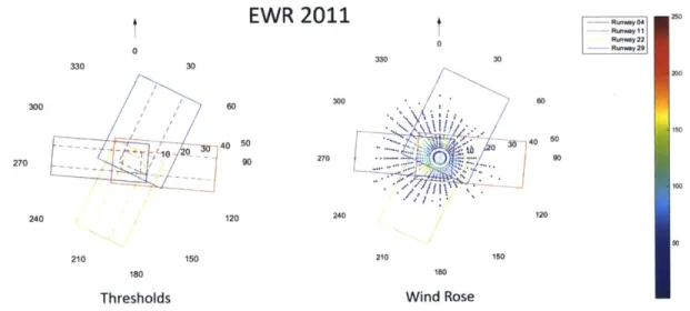
3.2.2 Wind speed, wind direction, and wind thresholds learned from year 2011 EW R data. . . . . 36

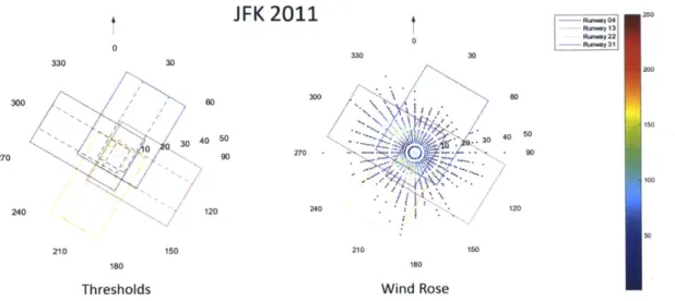
3.2.3 Wind speed, wind direction, and wind thresholds learned from year 2011 JFK data. . . . . 37

3.2.4 Wind speed, wind direction, and wind thresholds learned from year 2011 LG A data. . . . . 37

3.2.5 Wind speed, wind direction, and wind thresholds learned from year 2011 SFO data. . . . . 38

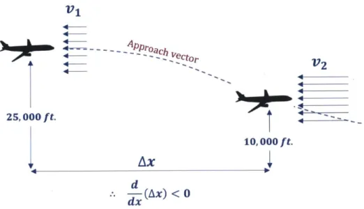
3.2.6 Diagram explaining aircraft compression upon arrival. . . . . 39 3.2.7 Temporal active arrival demand profile at EWR airport for year 2011. 40

3.2.8 Temporal active arrival demand profile at JFK airport for year 2011. 40

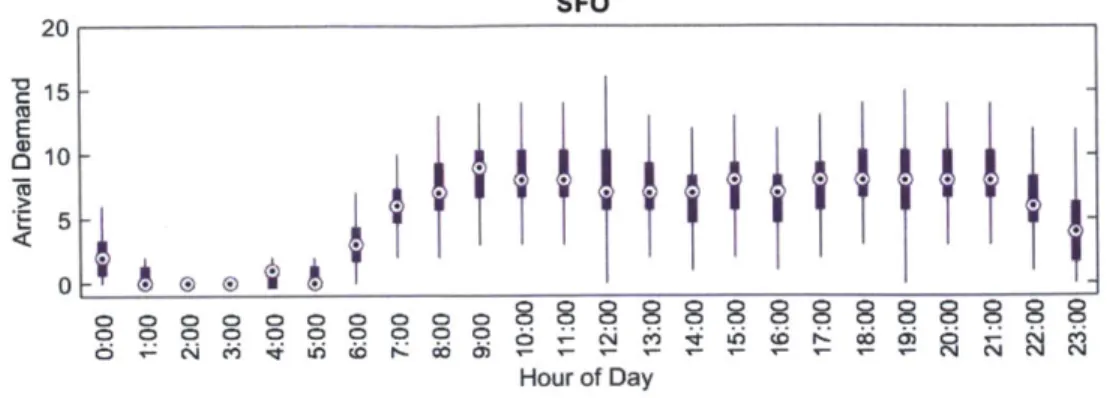
3.2.9 Temporal active arrival demand profile at LGA airport for year 2011. 40 3.2.10I'emporal active arrival demand profile at SFO airport for year 2011. 41

4.1.1 EWR model specification. . . . . 45

4.2.1 JFK model specification. . . . . 48

4.2.2 JFK Combined Configuration Model specification. . . . . 53

4.3.1 LGA model specification. . . . . 53

4.4.1 SFO model specification. . . . . 58

4.4.2 SFO AARs under VMC and IMC in 2011. . . . . 61

5.1.1 EWR classification confusion matrix for 3 hour time horizon (ASPM d ata ). . . . . 68

5.1.2 Comparison with baseline heuristic for EWR in 2012. . . . . 70

5.1.3 JFK classification confusion matrix for 3 hour time horizon (ASPM d ata). . . . . 72

5.1.4 Comparison with baseline heursitic for JFK in 2012. . . . . 73

5.1.5 LGA classification confusion matrix for 3 hour time horizon (ASPM data). ... ... 75

5.1.6 Comparison with baseline heuristic for LGA in 2012. . . . . 76

5.1.7 SFO classification confusion matrix for 3 hour time horizon (ASPM d ata ). . . . . 79

5.1.8 Comparison with baseline heuristic for SFO in 2012. . . . . 80

6.2.1 New York Metroplex Configuration Model specification. . . . . 86

6.2.2 NY Metro. Configuration classification confusion matrix for 3 hour time horizon (ASPM data). . . . . 90

6.3.1 NY Metro. Stacked Model classification confusion matrix for 3 hour time horizon (ASPM data). . . . . 93

6.3.2 Comparison between NY Metro. Configuration Model and NY Metro. Stacked Model when Configuration Model model predictions are correct. 96 6.3.3 Comparison between NY Metro. Config Model and NY Metro. Stacked Model when Stacked Model predictions are correct. . . . . 97

List of Tables

1.2.1 Frequent configurations observed at EWR, JFK, LGA, and SFO in year 2011. ...

1.2.2 Frequent New York Metroplex configurations in year 2011. . . . .

1.2.3 Combined NY Metro. configurations. . . . .

3.2.1 Runway angles at EWR, JFK, LGA, and SFO with respect to true

north and magnetic north. . . . .

3.2.2 Occurrences of 28R,28LI1R,1L and 28R/LI1R,1L at SFO in 2011. . .

4.1.1 Estimated utility function weights for EWR. . . . . 4.2.1 Estimated utility function weights for JFK - Part I. 4.2.2 Estimated utility function weights for JFK - Part II. 4.2.3 Estimated utility function weights for JFK - Part III. 4.2.4 Combined JFK configurations. . . . . 4.2.5 Estimated utility function weights for JFK's Combined M odel. . . . . 4.3.1 Estimated utility function weights for LGA - Part I. 4.3.2 Estimated utility function weights for LGA - Part II. 4.4.1 Estimated utility function weights for SFO . . . . .

Configuration

4.4.2 Estimated utility function weights for SFO utilities designating side-by and staggered. . . . .

5.1.1 Prediction accuracy (using actual weather and demand) for EWR in

2012.. .... ... . . ... . . . . 24 26 27 35 42 47 49 50 51 52 54 56 57 59 63 67

5.1.2 Prediction accuracy (using actual weather and demand) for JFK in 2012. 71 5.1.3 Prediction accuracy (using actual weather and demand) for LGA in

2012... ... 74

5.1.4 Prediction accuracy (using actual weather and demand) for SFO in 2012. 78

5.2.1 Prediction accuracy (using forecast weather and scheduled demand

data) for EW R in 2012. . . . . 82 5.2.2 Prediction accuracy (using forecast weather and scheduled demand

data) for LGA in 2012. . . . . 83 5.2.3 Prediction accuracy (using forecast weather and scheduled demand

data) for SFO in 2012. . . . . 84

6.2.1 Estimated utility function weights for New York Metroplex

Configura-tion M odel - Part I. . . . . 88 6.2.2 Prediction accuracy (using actual weather and demand) for NY Metro.

Configuration Model in 2012. . . . . 89 6.3.1 Prediction accuracy (using actual weather and demand) for NY Metro.

Stacked M odel in 2012.. . . . .. .. . .. . ... . . . . 92 6.3.2 Comparison between NY Metro. Configuration Model and NY Metro.

Stacked M odel predictions. . . . . 94

6.3.3 New York Metroplex Stacked Model statistics. . . . . 95

6.3.4 Confusion table comparing overall NY Metro. Configuration Model and NY Metro. Stacked Model. . . . . 96

Chapter 1

Introduction

Airport congestion leads to significant flight delays at the busiest airports around the world. Fundamentally, congestion is caused by an imbalance between demand (air-port operations) and supply (air(air-port capacity) within the air trans(air-portation system. Airport expansion projects can increase the runway capacity at an airport, but are expensive and take many years to complete; by contrast, the better utilization of ex-isting airport capacity is a less expensive approach to mitigating airport congestion. The key driver of airport capacity at a given time is the active runway configura-tion [1], which is the combinaconfigura-tion of runways being used to handle the arrival and departure flows at the airport under consideration.

When selecting a runway configuration, air traffic control personnel must con-sider meteorological and operational factors such as wind speed, wind direction, ar-rival demand, departure demand, noise mitigation, and inter-airport coordination.

A comprehensive understanding of the runway configuration selection process by air

traffic personnel is necessary for the future development of decision support tools under SESAR and NextGen initiatives. A keen understanding of this process has the potential to increase the operational efficiency of airport capacity utilization and provides a key step toward airport capacity prediction. Airport capacity predictions are important inputs needed for air traffic flow management [2, 3], airport surface operations scheduling [4], and system-wide simulations [5]. Since the capacity of an airport depends heavily on the runway configuration being used, the forecast of the

runway configuration is a key step toward predicting the capacity of an airport. This paper develops a data-driven model of the runway configuration selection pro-cess using a discrete-choice modeling framework for Newark (EWR), John F. Kennedy

(JFK), LaGuardia (LGA), and San-Francisco (SFO) airports. It also extends this

dis-crete choice approach to model the configurations of the entire New York Metroplex which includes EWR, LGA, and John F. Kennedy (JFK) airports. The models in-fer the utility functions that best explain (that is, maximize the likelihood of) the observed decisions. The utility functions give insight on the relative importance of the different decision factors to air-traffic control personnel when selecting a runway configuration. The resultant model yields a probabilistic prediction of the runway configuration at any time, given a forecast of the influencing factors.

1.1

Related Work

1.1.1

Prescriptive Models

Two types of models have previously been developed for the runway configuration selection problem: prescriptive and descriptive models. Prescriptive models account for the weather and other operational constraints to recommend an optimal runway configuration. An early example of a prescriptive model is the Enhanced Preferential Runway Advisory System (ENPRAS) that was developed for Boston Logan Interna-tional Airport (BOS) [6]. The ENPRAS was created to mitigate noise impacts from aircraft arrivals and departures at BOS and provide noise relief to nearby commu-nities by selecting optimal runway configurations (usually over water). The optimal configuration was determined considering weather, demand, and runway conditions. Both long-term aggregate noise pollution impacts and short-term impacts to nearby communities were considered when developing the system. So far, the ENPRAS has successfully helped operators at BOS lower the noise levels to surrounding communi-ties, and future implementations will help airport operators plan for optimal runway use over their entire shift period.

Also motivated by aircraft noise considerations, runway allocation systems were designed for Sydney and Brisbane airports [7]. These systems allowed for a more robust method for detecting aircraft noise profiles by using time-stamped aircraft movement composite-year data sets instead of the conventionally used day-average movement data sets. These new composite-year data sets were then tested within runway allocation models and was shown to predict the runway allocation at a higher level of confidence than previously used methods.

More recently, several authors have considered the problem of optimally schedul-ing runway configurations, takschedul-ing into account different models of weather forecasts and the loss of capacity during configuration switches [8, 9, 10, 11, 12]. Airports are assumed to operate under capacity envelopes that govern the amount of arrivals and departures that an be handled at an airport. These capacity envelopes directly depend on the runway configuration being used. High-level approaches using these concepts have attempted to describe the benefits to the entire National Airspace Sys-tem (NAS) when operating in a certain runway configuration. More recent approaches drill deeper and examine airports individually, focusing on their unique complexities and attributes to predict future runway configuration changes [12]. Additionally, models were also developed to determine the optimal relative sequencing of runway configurations by applying mixed integer programming models. These models were developed to reach an optimal balance of arriving aircraft and departing aircraft at an airport over time [11]. Other models dealt with capacity loss at an airport dur-ing a runway configuration switch, assigndur-ing transition penalties to mimic real-world operating conditions during a runway configuration switch [10].

1.1.2

Descriptive Models

Descriptive models use data-mining approaches to predict the runway configuration selection based on historical data. These models describe the decision selection pro-cesses of decision makers and use those propro-cesses to make predictions rather than simply recommending an optimal runway configuration. Descriptive models have re-ceived less attention than prescriptive models, but recently research in this field has

grown significantly. An example of a descriptive modeling approach uses data-mining methods to forecast Airport Arrival Rates (AARs) using Terminal Aerodrome Fore-cast (TAF) data. The TAF data is used to develop capacity profiles for airports using different stochastic approaches such as k-means clustering and dynamic time warping. A design of experiments methodology was taken by assigning the cost of delay to an objective function. The stochastic capacity profiles forecast AARs by minimizing the cost of delay objective function using the real-time data available to airport operators when making decisions. This methodology also makes the approach beneficial for Ground Delay Program (GDP) planning [14].

A 24-hour forecast of runway configuration was developed for Amsterdam Schiphol

airport using a probabilistic weather forecast [15]. The method used modified two-dimensional Gaussian distribution with wind speed and wind direction as degrees of freedom to develop probabilities of selecting a runway configuration. The intent of this model is to provide airport operators with decision support tools based on future weather forecasts. The model can also keep nearby civilians who live close to the airport informed of the likely impacts that weather will have on airport operations

- and in turn the noise over their communities. In some cases, these models achieve accuracies of up to 70%.

A logistic regression based approach was used to develop a descriptive model of

runway configuration selection at LGA and JFK, although this was not a predictive model [16]. These models have been shown to have accuracies of up to 75%, however, a difficult task has been modeling the observed resistance to configuration changes from air traffic control personnel. Recent research using discrete-choice models of the runway configuration selection process for year 2006 at EWR and LGA airports have taken this observation into account with similar accuracies [17, 18]. The model parameters in these discrete-choice models were set using standard operating proce-dures at EWR and LGA, which are subject to change and can sometimes disagree with the data.

1.1.3

Extension of Previous Work

This paper will extend the aforementioned discrete-choice models at EWR and LGA for years 2011-2012 with a more data-driven approach. The methodology will also be applied to SFO and JFK for years 2011-2012. Finally, the discrete-choice approach will be applied to the entire New York Metroplex for years 2011-2012. A key novelty in this paper is that the constraints pertaining to the maximum allowable tailwinds and crosswinds are learned from the actual data rather than the FAA operating manuals.

The utility functions within the discrete-choice framework capture the impor-tance of wind speed and direction, air traffic demand, noise abatement procedures,

and the coordination of flows with neighboring airports. An advantage of the discrete-choice approach is its ability to account for the resistance to configuration switches

by air-traffic control, called operational "inertia" in this paper. Switching a

run-way configuration requires increased coordination among airport stakeholders which lowers airport throughput, and consequently makes air traffic control personnel to resist frequent configuration changes. While the influence of inertia is arguably less important on long forecast horizons (when the key factors are likely to be wind con-ditions, visibility, and demand), the resistance to configuration changes play a much more prominent role on short forecast horizons (such as 3-hours ahead). Without accounting for inertia, tools that suggest possible choices for the optimal runway con-figuration recommend significantly more frequent changes than were seen in actual operations [12]. The discrete-choice modeling framework helps to accommodate the effect of inertia, in addition to the other influencing factors.

This paper illustrates the proposed approach using case studies for EWR, JFK,

LGA, SFO, and the New York Metroplex, first assuming a knowledge of the actual

weather conditions and the traffic demand 3 hours ahead, and then using the most recent Terminal Aerodrome Forecast (TAF) available 3 hours in advance.

1.2

Airports Considered

1.2.1

EWR

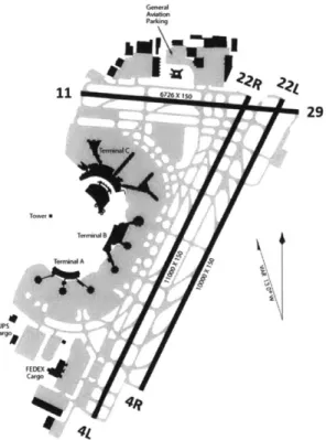
Newark Liberty Internal Airport is one of three major airports in the New York Metroplex. EWR handles approximately 35 million passengers a year on three run-ways: 4L/22R, 4R/22L, and 11/29 [19]. EWR serves as a hub for United Airlines, which handles approximately 70% of its passenger traffic [19].

An airport layout of EWR is shown in Figure 1.2.1. Typically, runway 4L/22R is used for departures and 4R/22L is used to handle arrivals. Runway 11/29 is not usually preferred because it is not capable of instrument landing approaches, however during very strong crosswinds runway 11/29 may be used to handle either arrivals or departures. 25 different runway configurations at EWR were reported in year 2011. Table 1.2.1 shows the frequencies with which the most commonly-used configurations at EWR were observed.

Aviation Purking 29 F fpI FEDEX

1.2.2

JFK

John F. Kennedy International Airport is another of the three major airports in the New York Metroplex. JFK handles approximately 55 million passengers a year and is operationally the largest international airport in the United States [20]. The airport serves as a hub for American Airlines, Delta Airlines, and JetBlue.

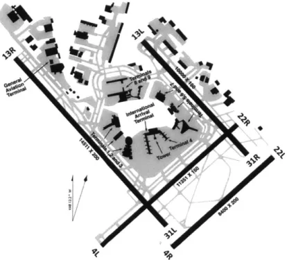
JFK has four runways: 13R/31L, 4R/22L, 4L/22R, and 13L/31R [21]. An airport

layout of JFK is shown in Figure 1.2.2. Commonly, arrivals are handled using runways 31L/13R or 4L/22R depending on the specific conditions, and departures are typically handled with 13R/31L. 43 different runway configurations at JFK were reported in 2011. Table 1.2.1 shows the frequencies with which the most commonly-used configurations at JFK were observed.

Ir

Figure 1.2.2: Layout of JFK airport.

1.2.3

LGA

LaGuardia Airport is the final major airport in the New York Metroplex. LGA handles approximately 25 million passengers a year on two runways: 4/22 and 13/31

[22]. LaGuardia acts as a hub for Delta Airlines.

An airport layout of LGA is shown in Figure 1.2.3. The active runways for arrivals and departures depends on the weather conditions, but typically, arrivals at LGA are handled on runway 4/22 and departures are handled on runway 13/31. 27 different runway configurations at LGA were reported in 2011. Table 1.2.1 shows the frequen-cies with which the most commonly-used configurations at LGA were observed.

Aviation

Figure 1.2.3: Layout of LGA airport.

1.2.4

SFO

San Francisco International Airport is the major airport in the San Francisco Bay Area, handling approximately 47 million passengers annually [23]. SFO acts as a hub for United Airlines and Virgin America.

As shown in Figure 1.2.4, SFO has four runways: 1OL/28R, 1OR/28L, O1L/19R, and O1R/19L [24]. Handling arrivals and departures at SFO is uniquely challenging for air traffic control because the centerlines of runways 10L/28R, and 1OR/28L are only separated by 750 feet. According to FAA regulations parallel approaches cannot be allowed during poor weather conditions at such a small separation. This effec-tively lowers the capacity of the airport during overcast weather, and will be shown

to present a significant modeling challenge in this paper. 24 different runway config-urations at SFO were reported in 2011. Table 1.2.1 shows the frequencies with which the most commonly-used configurations at SFO were observed.

Figure 1.2.4: Layout of SFO airport.

1.2.5

New York Metroplex

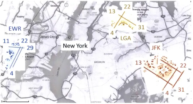
The New York Metroplex is comprised of three major airports within a relatively close proximity to another - EWR, JFK, and LGA. A map layout of the New York Metroplex is shown in Figure 1.2.5 In come cases, the large general airport TEB is included, but it will be left out for the purposes of this research. The New York Metroplex is a very large bottleneck on the NAS because it has the largest number

of arrival and departure operations in the United States [35, 36]. Consequently, it

is the most congested airspace in the NAS [34]. Delays that occur in the New York Metroplex propagate throughout the rest of the system and can have a heavy impact on the overall delay state of the NAS.

Prior research has suggested that the New York Metroplex is beginning to reach its maximum airspace capacity given the current operational landscape and physical

Table 1.2.1: Frequent configurations observed at EWR, 2011.

JFK, LGA, and SFO in year

Airport Configuration Frequency % Frequency

21L,11122R 4,214 13% 22LI22R 16,559 50% EWR 22LI22R,29 353 1% 4L,4R4L 528 2% 4R,1114L 1,576 5% 4R14L 10,221 31% 13L,22L113R 2,174 6% 13LI13R 1,395 4% 22L,22RI22R 2,579 7% 22L,22R122R,31L 1,785 5% 22LI22R 3,528 10% JFK 22L122R,31L 4,085 12% 31L,31RI31L 7,064 20% 31R131L 3,233 9% 4L,4RJ4L 1,927 5% 4L,4R14L,31L 1,987 6% 4R14L 2,592 7% 4R14L,31L 1,835 5% 22113 6,846 24% 22131 5,556 19% 22,31131 852 3% LGA 31131 2,676 9% 3114 7,608 26% 4113 4,113 14% 1 1 414 1,372 5% 19R,19LI10R,1OL 957 3% 28R,28L01R,01L 24,871 74% SFO 28R,28L128R,28L 3,000 9% 28R01R,01L 467 1% 28L101R,O1L 4,244 13%

layout of EWR, JFK, and LGA [32]. Because of the large expected increase in air travel demand over the next few decades, a major component of NextGen research has been devoted to examining possible capacity enhancements for the New York Metroplex. This paper will also model the New York Metroplex using a discrete choice approach. The utility functions learned from these models could help future models with capacity predictions or defining objective functions for decision support

29

Ne YorkJFK

222

_13OKY

₁₃

I

Figure 1.2.5: Layout of EWR, JFK, and LGA in the New York Metroplex.

tools.

Just as the previously mentioned airports were shown to have runway

configu-rations, the New York Metroplex is considered to have certain "configurations" as well. The New York Metroplex runway configurations are simply the combined run-way configurations of EWR, JFK, and LGA at any given time. By the nature of this definition, the New York Metroplex configurations switch much more often and have a lower number of occurrences compared to the configurations at each individual airport. Table 1.2.2 shows the most frequent

(filtered

As shown, in Table 1.2.2, many configurations seem similar to others and typically

occur less frequently than most of the individual airport configurations. For these reasons the New York Metroplex configurations are difficult to model. To help manage these difficulties, prior research used the configurations at each individual airport to develop overarching configurations for the New York Metroplex

[34].

Table 1.2.2: Frequent New York Metroplex configurations in year 2011.

NY Metro Config. ID EWR Config. JFK Config. LGA Config. Freq. % Freq.

1 11,22L122R 13L,22L113R 22113 565 1.6% 2 11,22L122R 22L122R,31L 22113 358 2.6% 3 22LI22R 13LI13R 22113 442 3.2% 4 22LI22R 22L,22R22R 22113 884 6.3% 5 22LI22R 22L,22RI22R,31L 22131 628 4.5% 6 22LI22R 22LI22R 22113 1,149 8.2% 7 22L|22R 22LI22R 22131 516 3.7% 8 22LI22R 22LI22R,31L 13,22113 368 2.6% 9 22LI22R 22L122R,31L 22113 1,061 7.6% 10 22L122R 22L122R,31L 22131 739 5.3% 11 22LI22R 31L,31RI31L 22131 1,060 7.6% 12 22LI22R 31L,31R31L 31131 392 2.8% 13 22LI22R 31L,31RI31L 3114 416 3.0% 14 22L|22R 31R131L 22131 356 2.5% 15 4R,1114L 31L,31RI31L 3114 518 3.7% 16 4R14L 31L,31RI31L 3114 1,273 9.1% 17 4R14L 31RI31L 3114 580 4.2% 18 4R14L 4L,4R14L 4113 750 5.4% 19 4R14L 4R14L 3114 425 3.0% 20 4R14L 4R14L 4113 623 4.5% 21 4R14L 4R14L,31L 3114 487 3.5% 22 4R14L 4R14L,31L 4113 371 2.7%

Southern aircraft flow under Southern aircraft flow under I

Southern aircraft flow under

Mixed southern and northern Mixed southern and northern Northern aircraft flow under Northern aircraft flow under I Northern aircraft flow under

VMC MC. VMC flow flow VTMC MC. VfMC

with an arrival priority.

with a departure priority.

with an emphasis on northern flow.

with an emphasis on southern flow.

with an arrival priority.

with a departure priority.

The overarching New York Metroplex configurations and their components are shown in Table 1.2.3. 1. 2. 3. 4. 5. 6. 7. 8.

Table 1.2.3: Combined NY Metro. configurations.

NY Metro Config. ID EWR Config. JFK Config. LGA Config. Freq. % Freq.

1 11,22LI22R 13L,22L113R 22113 565 1.6%

3 22LI22R 13LI13R 22113 442 3.2%

South Flow - VMC - Arrival Priority (S-VMC-AP) 2,794 20%

2 11,22L122R 22L122R,31L 22113 358 2.6%

4 22LI22R 22L,22R122R 22113 884 6.3%

6 22L122R 22LI22R 22113 1,149 8.2%

8 22LI22R 22L122R,31L 13,22113 368 2.6%

9 22LI22R 22L122R,31L 22113 1,061 7.6%

South Flow -IMC (S-IMC) 1 2,033 14.6%

5 22LI22R 22L,22R122R,31L 22131 628 4.5%

7 22LI22R 22L1,22R. 22131 516 3.7%

10 22LI22R 22L122R,31L 22131 739 5.3%

South Flow - VMC - Departure Priority (S-VMC-DP) 1,883 13.5%

11 22LI22R 31L,31R31L 22131 1,060 7.6%

14 22LI22R 31RI31L 22131 356 2.5%

Mixed North and South Flow with South Emphasis (Mixed S to N) 1,416 10.1%

12 22LI22R 31L,31R31L 31131 392 2.8%

13 22LI22R 31L,31R31L 3114 416 3.0%

Mixed North and South Flow with North Emphasis (Mixed N to S) 808 5.8%

15 4R,1114L 31L,31RI31L 3114 518 3.7%

16 4R14L 31L,31R31L 3114 1,273 9.1%

17 4R14L 31R131L 3114 580 4.2%

North Flow - VMC -Arrival Priority (N-VMC-AP) 2,371 17.0%

18 4R14L 4L,4R14L 4113 750 5.4%

20 4R14L 4R14L 4113 623 4.5%

22 4R14L 4R14L,31L 4113 371 2.7%

North Flow - IMC (N-IMC) 1,744 12.5%

19 4R14L] 4R14L 3114 425 3.0%

21 4R14L 4R14L,31L 3114 487 3.5%

North Flow - VMC - Departure Priority (N-VMC-DP) 912 6.5%

1.3

Notation

Runway configurations are typically designated in the form of 'Al,A2 I D1, D2' where

Al and A2 are the arrival runways, and Dl and D2 are the departure runways. The

numbers for each active runway are reported based on their bearing from magnetic north (in degrees) divided by 10. Pairs of parallel runways are differentiated by 'R' and 'L'. For instance, if Newark, shown in Figure 1.3.1, is operating in runway

configuration 22LI22R, aircraft arrivals are handled on runway 22L which faces 220 degrees from magnetic north and departures are handled on parallel runway 22R which also faces 220 degrees from magnetic north.

Theoretically, an airport with N runways has O(6N) possible configurations, since each runway can be used for arrivals, departures or both, and in either direction. Throughout a year, many different runway configurations are seen, however, typically

5-10 runway configurations are used the majority of the time. In addition, due to the

additional coordination required during switches, runway configurations only change

1-3 times per day on average.

29

41

22L|22R

Chapter 2

Methodology

2.1

Discrete-Choice Modeling Framework

Discrete-choice models are behavioral models that describe the choice selection of a decision maker, or the nominal decision selection among an exhaustive set of possible alternative options, called the choice set

[26].

The utility function is modeled as stochastic random variable, with an observed (deterministic) component, V, and a stochastic error component, 6. For the nth

selection, given a set of feasible alternatives Cs, the utility of choice ci

E

represented as

Un,i = Vn,i + 6ri. (2.1.1) The decision maker selects the alternative with maximum utility, that is, cj E Cn such that

j

i:ciECn

The observable component of the utility function is defined as a linear function of the observed vector of attributes, Xn,,. The attributes include the different factors

include alternative specific constants, an,,, as follows:

Vn' i = an'i + [On,3 - Xn,i]. (2.1.3)

The random error component of the utility function reflects all measurement er-rors, including unobserved attributes, variations between different decision-makers, proxy variable effects, and reporting errors. The error term is assumed to be dis-tributed according to a Type I Extreme Value (or Gumbel) distribution with a

loca-tion parameter of zero, that is:

f(x)

function are independent from one another, as shown in Figure 2.1.1.

Decision

Alt.

1

Alt. 2

Alt. 3

Alt. 41

Alt. 5

Figure 2.1.1: Example of a MNL model structure.

Under the assumptions of the MNL model, the probability that choice i is chosen during the rIth selection is given by

P"' .= (2.1.5)

Pnci E~ CCn 'C

The independence among the error terms of each utility function in the MNL model assumes that all correlation among alternatives has been captured by the attributes included in the utility function [26]. The Nested Logit (NL) model relaxes

this assumption by grouping alternatives into subsets, or nests (denoted Bk), which have correlation between their error terms (Figure 2.1.2).

Decision

Nest I

Nest 1

AAtA.

4

A

Figure 2.1.2: Example of a NL model structure.

The NL model splits the observable part of the utility function into a component that is common among the alternatives within a nest, and a component that varies between the different alternatives in a nest. The NL model can then be treated as nested MNL models using conditional probabilities. The probability that a specific alternative is chosen is given by the probability that its nest is chosen, multiplied by the probability that the specific alternative is chosen from among the alternatives in that nest. In other words

Pn (ci) =Pn(cilBk)Pn(Bk), (2.1.6)

where Pn(Bk) = (2.1.7)

ZEjBk fexp(PkVn,j)]

In,k Iln(Z exp([ukVn,i)). (2.1.9)

I-k _j(EBk

Equation (2.1.7) has an additional term in the numerator called the inclusive value, that acts as a bridge between the "lower level MNL structures" within each

2.2

Maximum-Likelihood Estimation of Model

Pa-rameters

Maximum-likelihood estimates of the linear weighting parameters, alternative specific constants, and scale parameters are estimated from the training data. The maximum-likelihood function is defined as the joint probability that the vector of sample data will occur, given a vector of parameters 0 =< a, /, p.> as follows,

L(O) = P(X; 0). (2.2.1)

The estimated parameters are those that maximize the likelihood of the observa-tions:

(a, 3,

/l)

The resulting nonlinear optimization problem is solved computationally using an open-source software package called BIOGEME [27].

2.3

Statistical Tests

The discrete-choice models for EWR, JFK, LGA, SFO, and the New York Metroplex were realized iteratively, adding or removing variables based on their statistical signif-icance as determined by the Students t-test. The signifsignif-icance of each attribute to the overall model was tested using likelihood ratio testing. Different nested logit model tree structures were also evaluated for statistical significance using likelihood-ratio testing [26].

Chapter 3

Pre-processing The Data

3.1

Training and Testing Data

The training and test datasets for each airport were taken from the FAA's Avia-tion System Performance Metrics (ASPM) database [28]. The data is reported in 15-minute intervals and includes the active runway configuration, the arrival and departure demand, cloud ceiling, visibility conditions, wind speed, and wind direc-tion. Training data for SFO, LGA, and EWR was taken from year 2011 and the test datasets were taken from year 2012. Results from the prediction models that use

ASPM test data assume perfect knowledge of the wind, visibility, and demand for

the subsequent three hour interval. Test data sets will also be created using Terminal Aerodrome Forecast (TAF) data and schedule demand data which does not assume precise knowledge of the weather and demand over the next three hours. Predic-tion results using the TAF and schedule demand data effectively simulate predicPredic-tions using data that air traffic control personnel would have in real time.

3.2

Attribute Selection

The utility function is assumed to be a linear function of the observed vector of at-tributes, or factors, that influence the decision. For the runway configuration selection

3.2.1

Inertia

During a runway configuration switch it is necessary to have increased coordination among all stakeholders (airlines, air traffic control, ground operations,etc.), which reduces the airport throughput [111. Operational "inertia" is a term used to describe the preference of air traffic control to resist runway configuration changes, due to the high operational effort required during the switch. Tools designed to suggest an optimal runway configuration have been shown to recommend significantly more frequent runway configuration switches than is actually observed in practice. An inertia variable was added as an attribute in the models to reflect the preference of air traffic controllers to resist configuration changes. The inertia variable adds a positive contribution to the utility function of the incumbent configuration.

3.2.2

Wind Speed and Wind Direction

Wind speed and direction are key factors that influence the choice of runway configura-tion. High tailwinds and crosswinds are operationally unsafe in many circumstances, and as a result, render certain runways unusable. The Federal Aviation Administra-tion (FAA) has specified the maximum allowable tailwind and crosswind thresholds for the safe operation of a runway in standard operating procedures (SOPs). Prior work on runway configuration selection based runway availability on SOPs in the model. In this paper, the threshold values of runway tailwinds and crosswinds are directly backed out of the ASPM year 2011 training data sets for each airport.

The ASPM dataset gives both the wind direction with respect to true north, 0 and wind speed, v, for each 15-minute interval. Figure 3.2.1 illustrates that the headwind

and crosswind components are given by,

Headwind = v cos( o - 0) (3.2.1)

Crosswind = v sin(o - 6) (3.2.2)

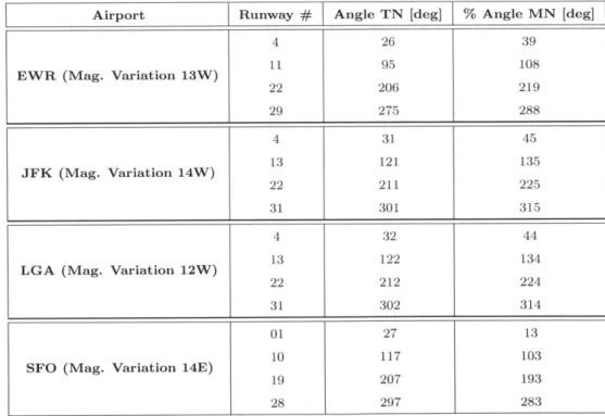
that p does not correspond to the angle implied by the runway number, which is given with respect to magnetic north. The runway angle relative to true north is calculated

by adding an offset that depends on the geographic location of the airport, shown in

Table 3.2.1. Tailwinds occur when the headwind function takes a negative value.

Figure 3.2.1: Determination of the headwind and crosswind components.

Table 3.2.1: Runway angles at EWR, JFK, LGA, and SFO with respect to true north and magnetic north.

Airport Runway # Angle TN [deg] % Angle MN [deg]

4 26 39

11 95 108

EWR (Mag. Variation 13W)

22 206 219 29 275 288 4 31 45 13 121 135 JFK (Mag. Variation 14W) 22 211 225 31 301 315 4 32 44 13 122 134

LGA (Mag. Variation 12W)

22 212 224

31 302 314

01 27 13

10 117 103

SFO (Mag. Variation 14E)

19 207 193

28 297 283

Figures 3.2.2, 3.2.3, 3.2.4, 3.2.5 show the identified and wind direction for each runway at EWR, JFK,

ranges of feasible wind speed

LGA, and SFO respectively.

year 2011 at these airports. The identified ranges of tailwind and crosswind values for runway feasibility were learned directly from the 2011 ASPM data and are also shown on the plot. Note that air traffic controllers prefer headwinds to tailwinds and crosswinds, and while there is no headwind threshold for runway feasibility, headwind thresholds were plotted at 40 knots in the diagrams for better illustration. The tailwind and crosswind limits were taken on a "per-runway" basis, and were calculated via the following procedure.

1. Aggregate all tailwind and crosswind values for each runway at EWR, JFK, LGA, and SFO.

2. For each runway list, remove tailwind and crosswind combinations from time periods when the active configurations did not include any operations on the runway.

3. Take tailwind thresholds at 90th percentile and crosswind thresholds at the

95th percentile to remove possible reporting errors. In the plots, the solid line corresponds to the aforementioned thresholds for each runway, and the dashed lines correspond to the 75th percentile.

EWR 2011 _unw..0. 2 0 ~~-Runwey22 0 0 Runm0291 330 30 330 130 306 0 300 60 270 0 jj~~iII j -j100 240 120 240 120 so 210 150 210 150 180 180

Thresholds Wind Rose

Figure 3.2.2: Wind speed, wind direction, and wind thresholds learned from year 2011 EWR data.

JFK 2011 0 330 30 300 80 2 30 40 g0 270 - ~ 90 240 210 150 180 Thresholds

Figure 3.2.3: Wind speed, 2011 JFK data. 120

t

wind direction, and wind thresholds learned from year

4 330

LGA 2011

t

Figure 3.2.4: Wind speed, wind direction, and wind thresholds learned from year 2011 LGA data. R-,we04 - Runay 31 60 40 So 90 120 210 50 200 150 100 0 210 150 180 Wind Rose

SFO 2011 0 Runoey 19 30 0 - Rummy2 3 330 30 330 30 505 3 3 40 50 30 400 270 90 270 90 240 120 240 1120 100 210 150 210 150 so 180 10

Thresholds Wind Rose

Figure 3.2.5: Wind speed, wind direction, and wind thresholds learned from year 2011 SFO data.

The available choice set during a given selection period can change in a discrete choice framework. Even with the maximum tailwind and crosswind limitations, sev-eral runway configurations may be feasible at any time. Runway feasibility was used to directly govern the available subset of runway configurations in the discrete choice model during each time interval. If the wind speed and wind direction combination fell outside any of the thresholds for a runway, all configurations using that runway were removed from the available choice set during the given decision selection period. Figures 3.2.2, 3.2.3, 3.2.4, and 3.2.5 show that the majority of points correspond to conditions in which all the runway configurations are considered feasible.

Headwinds are expected to add a positive contribution to the utility functions and tailwinds are expected to add a negative contribution. Significantly high headwinds, however, could potentially have an adverse effect on airport operations by decreasing the space between aircraft arrivals during landing - a phenomenon known as com-pression [29]. Shown in Figure 3.2.6, comcom-pression occurs when there are significantly higher headwinds near the ground than at cruise altitude during the arrival approach.

If the ground headwinds are high enough, the relative spacing between consecutive

arrivals will begin to decrease as the flights begin their descent toward the airport, which can cause safety problems and congestion.

V1 )h~I~uum~ _Approach6 ! ctor 25, 000 ft. 4-

Ax

Figure 3.2.6: Diagram explaining aircraft compression upon arrival.

To account for the effects of compression, headwinds above the 85th percentile were treated as "high headwinds". Variables for "normal headwinds" (below the

85th percentile) and "tailwinds" were added to each model as well.

3.2.3

Demand

Airport arrival and departure demand play a significant role when selecting the run-way configuration. Specifically, in high demand situations, high capacity configura-tions are preferred. These typically include an extra arrival or departure runway.

Figures 3.2.7, 3.2.8, 3.2.9, and 3.2.10 show the active arrival demand variation throughout the time of day at EWR, JFK, LGA and SFO airports during year 2011. Demand typically peaks around 9:00 - 11:00 AM because it is the most convenient time

to arrive for business travel. Because of the time-dependence of arrival demand at each airport, adding demand into the utility functions of the runway configurations also brings time-of-day effects into the model. One would assume that if demand typically peaks at an airport during a certain time of day, the high capacity configurations are more likely to be used during that time of day.

EWR

ii it4 4* 44 * 4H 4 4y

Hour of Day

Figure 3.2.7: Temporal active arrival demand profile at EWR airport for year 2011.

JFK 88 0 0 0 0 0 0 0 0 0 0 0 0 0 0 0 0 0 0 0 0 O N C'~~ ~* It~ CO t- COO~ Hour of Day

Figure 3.2.8: Temporal active arrival demand profile at JFK airport for year 2011.

20 15 E o10 5 0 LGA -M 4 *k Da 8(b i6 d -v -, V - 00000000 8o8 8 Hour of Day

Figure 3.2.9: Temporal active arrival demand profile at LGA airport for year 2011.

20 15 E 0 10 .~5 0 20 15 E o 10 .~5 0

SFO 20 15 E o10

>.

_5f

Figure 3.2.10: Temporal active arrival demand profile at SFO airport for year 2011.

3.2.4

Noise Abatement Procedures

Noise abatement procedures are used at many major airports to reduce the impacts

of noise on communities in the vicinity of the airport, especially during early morning

and nighttime hours. At EWR, JFK, and LGA, configurations with flight paths

over the city and away from populated areas are preferred during the nighttime. At

SFO, runway configurations that arrive and depart over the water are preferred to configurations that fly over populated areas. Variables were included in each model

to account for these effects.

3.2.5

Cloud Ceiling and Visibility

Meteorological conditions, as represented by the cloud ceiling and visibility, are

im-portant considerations for air traffic control personnel when selecting the runway

con-figuration. Visual Meteorological Conditions (VMC) refer to times when the visibility

is sufficient for pilots to maintain visual separation from the ground and other aircraft.

Instrument Meteorological Conditions (IMC) refer to times when pilots are required

to use their flight instruments. IMC is defined by a visibility less than 3 miles and a ceiling less than 1,000 feet [30]. The runway configuration selection could depend on whether VMC or IMC is implemented. The EWR and LGA models incorporates

variables for each utility function corresponding to visual and instrument conditions.

In this manner, these variables will capture any preferences for one configuration over

The optimal capacity configuration at SFO is 28R,2811R,1L. The runways used in this operation are closely-spaced at 750 feet apart. As per FAA regulations, si-multaneous arrivals are not allowed under IMC [30]. Therefore, one would expect that the 28R11R,1L or 28L11R,1L configurations (which involve using only one of the two runways for arrivals) would be favored under IMC. Table 3.2.2 shows the relative use of each of these configurations under VMC and IMC. As shown, even though the single arrival runway configurations are used a greater fraction of the time in IMC than in VMC, the runway configuration 28R,28L11R,1L is still used a majority of the time in IMC. During IMC, simultaneous "side-by" landings are not possible, and the airport operates as if it would be in a single arrival runway configuration using a "staggered" arrival approach. Operationally, the staggered 28R,281,1R,1L configura-tion under IMC may have a small capacity benefit over the 28RI1R,1L and 28LI1R,1L configurations. In order to evaluate these effects, new variables that combine the ef-fects of visibility and demand were used in the SFO model. Four categorical variables were defined for periods of:

1. IMC + low demand,

2. IMC + high demand,

3. VMC + low demand,

4. VMC + high demand,

where a low demand period was defined as less than 5 arrivals per 15-minute period and high demand was defined as greater than 8 arrivals per 15-minute interval.

Table 3.2.2: Occurrences of 28R,28L11R,1L and 28R/L11R,1L at SFO in 2011.

Configuration VMC IMC 28R,28LI1R,1L 19,832 (82.7%) 4,161 (17.3%)

28R/LI1R,1L 3,466 (65.3%) 1,844 (34.7%)

3.2.6

Coordination With Surrounding Airports

The four airports in the New York Metroplex - Newark (EWR), John F. Kennedy International Airport (JFK), LaGuardia (LGA), and Teterboro (TEB) - are all in

a very close proximity to one another. Air traffic controllers at each airport must therefore coordinate their aircraft arrival and departure flows with the other neigh-boring airports. In the EWR and LGA individual airport models, the impacts of TEB are ignored and categorical variables were added to account for operations at

JFK. JFK was chosen because of its large volume of operations, which was expected

to have a significant impact on the runway configurations at EWR and LGA. The

JFK discrete-choice model includes coordination variables for both EWR and LGA,

but also ignores the impacts from TEB.

3.2.7

Switch Proximity

If the airport conditions necessitate a runway configuration switch, certain

configu-ration switches require more coordination from airport stakeholders than others. For instance, the addition of an extra arrival runway may be easier to implement than a complete reversal in the direction of operations. To account for these effects, variables were added to weight each utility function differently depending on the previous con-figuration. The switch proximity variables are fundamentally the same as the inertia variables, but are applied only to the utility functions of the runway configurations that were not seen in the previous time interval instead of the incumbent configura-tion. In this sense, they do not account for the low likelihood of switching between two runway configurations that require a high amount of operational effort once the decision to switch the configuration has been made.

3.2.8

New York Metroplex Model Data Processing

The New York Metroplex model uses slightly different definitions than the attributes mentioned above. Since each overarching New York Metroplex configuration consisted of several different runway configurations at multiple airports, runway availability plays a much smaller role than it does in the individual airport models. The wind parameters were processed to align with the primary flow of arrivals and departures (i.e. North or South flow). Arrival and departure demand variables were taken as

the total arrival or departure demand from EWR, JFK, and LGA. Additionally, the VMC/IMC classifiers from EWR, JFK, and LGA were all averaged to create an overall New York Metroplex VMC/IMC classifier. The averaging allows the utility bonus or penalty to be reduced for a New York Metroplex configuration if EWR,

JFK, and LGA are not all in VMC or IMC.

3.3

_{Runway Configuration Filtering}

Runway configurations that were seen less than 1% of the time throughout the year were removed at EWR, JFK, and SFO to reduce possible reporting errors or cases of special operations that would make it difficult to reliably estimate the weights and predict with the models. For LGA, the filter was set to 2% for the individual airport model to further help reduce reporting errors that occurred during nighttime hours. Similarly, the New York Metroplex configuration model uses a 1% cutoff.

Chapter 4

Estimated Discrete-Choice Utility

Functions

4.1

EWR

EWR

22L,1122 2222R2R 22L 12211,29 Arrival on 4

4R,4LI4L 4R,114L 4Rj4L

Figure 4.1.1: EWR model specification.

In the EWR model, configurations were removed if they were not seen at least

1% of the decision selection periods throughout the year. Many model structures

were tested, and the final final model was chosen as a nested logit structure with nest containing all alternatives using runway 4 for arrivals with a scale parameter of

PAr,4 = 1.22, shown in Figure 4.1.1.

The estimated weighting parameters for the utility function for the EWR model are shown along with their standard errors and t-statistics in Table 4.1.1. Any