HAL Id: hal-02989509
https://hal.inria.fr/hal-02989509
Submitted on 7 Nov 2020
HAL is a multi-disciplinary open access
archive for the deposit and dissemination of
sci-entific research documents, whether they are
pub-lished or not. The documents may come from
teaching and research institutions in France or
abroad, or from public or private research centers.
L’archive ouverte pluridisciplinaire HAL, est
destinée au dépôt et à la diffusion de documents
scientifiques de niveau recherche, publiés ou non,
émanant des établissements d’enseignement et de
recherche français ou étrangers, des laboratoires
publics ou privés.
Ant collective cognition allows for efficient navigation
through disordered environments
Aviram Gelblum, Ehud Fonio, Yoav Rodeh, Amos Korman, Ofer Feinerman
To cite this version:
Aviram Gelblum, Ehud Fonio, Yoav Rodeh, Amos Korman, Ofer Feinerman. Ant collective cognition
allows for efficient navigation through disordered environments. eLife, eLife Sciences Publication,
2020, 9, �10.7554/eLife.55195�. �hal-02989509�
Ant collective cognition allows for efficient navigation through
1
disordered environments
2
Aviram Gelblum, Ehud Fonio, Yoav Rodeh, Amos Korman*, Ofer Feinerman*
3
November 7, 2020
4
* Co-Corresponding authors: Ofer Feinerman and Amos Korman
5
6
The cognitive abilities of biological organisms only make sense in the context of their
en-7
vironment. Here, we study longhorn crazy ant collective navigation skills within the context
8
of a semi-natural, randomized environment. Mapping this biological setting into the
‘Ant-in-a-9
Labyrinth’ framework which studies physical transport through disordered media allows us to
10
formulate precise links between the statistics of environmental challenges and the ants’ collective
11
navigation abilities. We show that, in this environment, the ants use their numbers to collectively
12
extend their sensing range. Although this extension is moderate, it nevertheless allows for
ex-13
tremely fast traversal times that overshadow known physical solutions to the ‘Ant-in-a-Labyrinth’
14
problem. To explain this large payoff, we use percolation theory and prove that whenever the
15
labyrinth is solvable, a logarithmically small sensing range suffices for extreme speedup.
Over-16
all, our work demonstrates the potential advantages of group living and collective cognition in
17
increasing a species’ habitable range.
18
19
Movement and navigation are key ingredients in the ecology of any animal species [1]. Within its
envi-20
ronment an animal may encounter diverse and unpredictable navigational challenges. In some cases, such as
21
chemotaxis, a simple biased random walk strategy suffices for efficient navigation [2]. However, when challenges
22
are complex [3], the animal may need to exploit cognitive tools [4] such as active sensing of the environment
23
[5], processing of gathered information [3], and memory formation [6]. Indeed, an animal’s navigation strategies
24
reflect both the structure and statistics of its environment [7] and its cognitive capacities [8], [9].
25
Cooperation is a common means by which animals may increase their cognitive capacity [10]. Group living
26
animals may improve their navigational choices through social learning [11], collective decision making [12],
27
[13], and leadership [14]. Whether these forms of collective cognition enable a species to broaden the range of
28
navigational challenges it can overcome [10] is an intriguing question.
29
We approach this question within the context of cooperative transport [15] by longhorn crazy ants
(Para-30
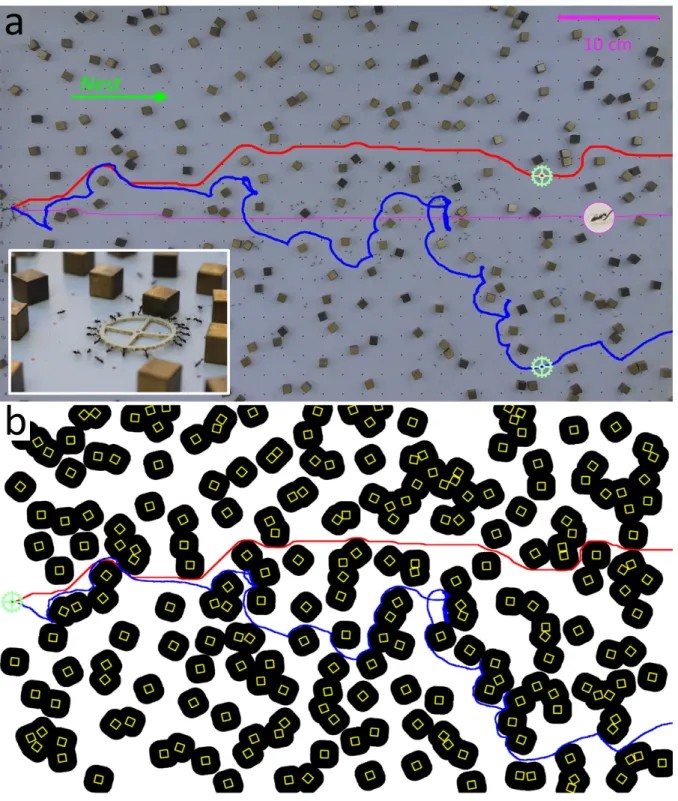
Figure 1: Motion within a maze. (a) Setup for cube maze experiments. Overlaid are the load trajectory (blue), shortest path for the load (red) and shortest path for ants (magenta). Inset shows a close-up image of the ring-shaped load as it is carried by ants through the cube maze. (b) Cube coverage of the maze shown in (a). Black regions are areas that are inaccessible to the load’s center, taking into account its radius. Cube coverage is defined as the fraction of inaccessible areas (Appendix 1.1, figure 1 supplement 1a). The load is marked in pale green and shown at its initial location. Shortest available path for the load is plotted in red and the ants’ actual trajectory is drawn in blue, as in (a).
trechina longicornis) [16]. To capture the structure and diversity of natural environmental conditions we track
31
groups of ants as they cooperatively transport large objects through semi-natural environments which mimic
32
random stone-riddled terrains. The inherent randomness of this setting produces a wide distribution of
nav-33
igational challenges that facilitates a study of the connections between individual capabilities, environmental
34
statistics, and emergent collective cognition [17].
35
An additional advantage of considering disordered environments is that motion through such environments
36
has been extensively studied from a physics and mathematical perspective [18]. Namely, percolation theory
37
studies the structure of porous or disordered media by modelling them as discrete or continuous [19] randomly
38
connected networks [20]. The percolation threshold of a network specifies the degree of connectivity at which
39
it undergoes a phase transition. Below the threshold, connections are few and the system breaks into small
40
disconnected clusters. Above the threshold, there are enough connections to form a single giant component
41
which spans the entire system. The ’Ant-in-a-Labyrinth’ framework [19]–[27] studies physical flows through
42
porous media by considering the motion of a biased random walker across percolation networks. Importantly,
43
while in these physical settings the dynamics are memoryless and governed by purely local forces, biological
44
systems are not necessarily limited by these constraints; animal navigation employs memory [28] and may
45
include non-local strategies such as collective sensing [29] or pheromone trails [30]. The ‘Ant-in-a-Labyrinth’
46
framework therefore allows for an interesting comparison between the performances of passive physical systems
47
and cognitive biological systems.
48
Results
49
Ants-in-a-Labyrinth
50
Semi-natural labyrinths were created by randomly spreading uniform sized cubes (0.8 by 0.8 cm2) across
51
a planar arena (70 by 50 cm2) bounded from 3 directions and open towards the nest (see figure 1). The ants
52
were initially recruited into the maze arena using cat food morsels, until a clear trail was established to the
53
initial load location near the center of the board’s edge that is furthest from the entrance (see figure 1b). The
54
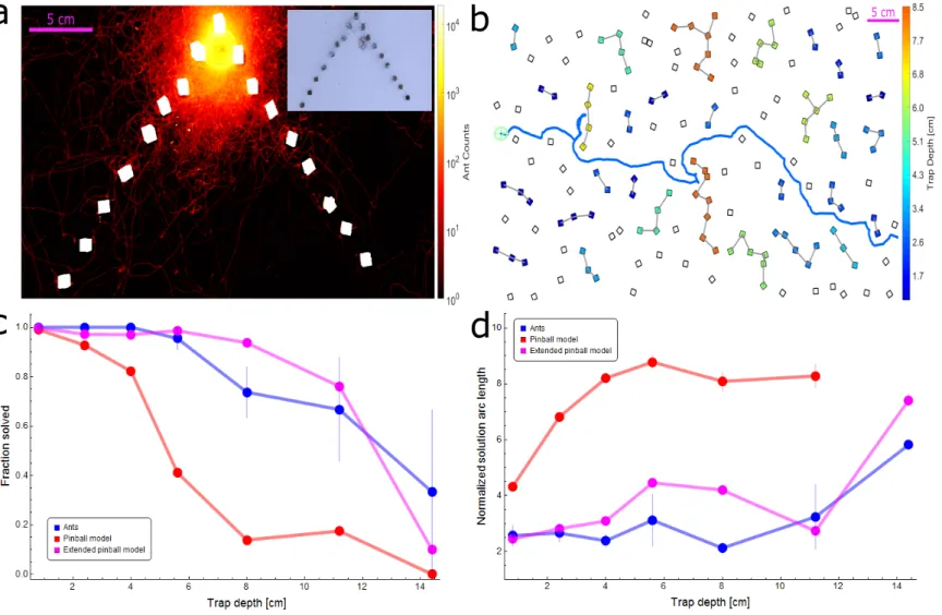
cat food morsels were then removed and instead a large food-like item (1 cm radius silicon ring) was placed on
55
the edge of the arena furthest from the entrance to the ants’ nest (See materials and Methods). This artificial
56
load was made attractive to the ants by storing overnight in a closed bag of cat food [14]. The ants were then
57
allowed to carry the food without any external intervention. Each maze configuration was tested once, before
58
repeating the process of maze creation, recruitment, and carrying.
59
In order to deliver the load to the nest, the ants had to cooperatively transport it amid cubes which often
60
interconnect into composite obstacles (see Movie 1). These obstacles generally interfere with the motion of
61
the large load but are effectively transparent to individual ants that can easily pass in the small gaps between
62
adjacent cubes [31] (figure 1a). This discrepancy makes escaping local traps and consequently finding a winding
63
trajectory that crosses the labyrinth highly non-trivial (figure 1).
64
The entire carrying process was filmed and the coordinates of the load, ants, and cubes extracted using
65
image processing (See Materials and Methods, Source data 1-2).
66
A labyrinth was declared to be solved if the load reached the edge of the arena closest to the nest within
67
an 8 minute time frame. By comparison, in the absence of cubes, the load traverses the same distance in a
68
mean time of less than 1.5 minutes. In the language of percolation theory, higher cube coverage (see figure
69
1b, Appendix 1.1, figure 1 supplement 1a) corresponds to reduced connectivity between the regions that are
70
available to the load’s motion. Low and intermediate cube densities that correspond to a connectivity level
71
above the percolation threshold yield soluble mazes. As cube density grows, the intricacy of the maze rises; this
72
manifests in a reduction in connectivity of the allowed regions, as the percolation threshold is approached. At
73
a certain high enough cube coverage, the labyrinth falls below its percolation threshold. This is accompanied
74
by the formation of large composite obstacles that break the labyrinth into disconnected islands which render it
75
insoluble. We find that the performance of the ants decreases with the number of cubes comprising the maze:
76
sparse mazes were more likely to be solved, were crossed faster, and with a shorter trajectory arc length (figure
77
2b-c, Appendix 2-figure 2b). The ants were able to solve mazes up to cube coverage of 55% (300 cubes). This
78
number is not far from the percolation threshold of this system, which occurs at 60% coverage, and beyond
79
which there is a sharp decrease in the number of solvable mazes (see Appendix 1.2, figure 1 supplement 1b).
80
Ants outperform biased random walks
81
To evaluate the ants’ performance under the percolation threshold we compared it to simpler, non-biological
82
models of motion in which the ants’ attraction to the nest is mapped to a directional bias. Specifically, we
83
introduce the pinball model as a continuous version of the discrete biased random walk. This model describes
84
the viscous motion of a ring that falls through an array of square pegs [32] in the presence of Brownian noise
85
(see Materials and Methods). Notably, the pinball model significantly outperforms the discrete biased random
86
walk (see Materials and Methods, Appendix 2-figure 2c). This improved performance stems from the fact that,
87
unlike the biased random walk which can stall at any obstacle, the falling ring quickly bypasses isolated pegs
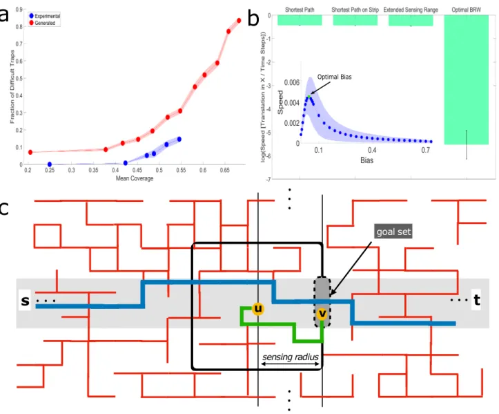
88
by rolling over them. Similar rolling behavior is also evident in the ants’ collective motion (Appendix 1.3 and
89
Appendix 1-figure 1) [33].
90
The free parameters of the pinball model were fit so that its simulated trajectories (see [34]) reproduce
91
major features of the ants’ collective motion in the absence of cubes (see Materials and Methods). Fixing
92
these parameters, the simulation was then run over all cube configurations as extracted from the experimental
93
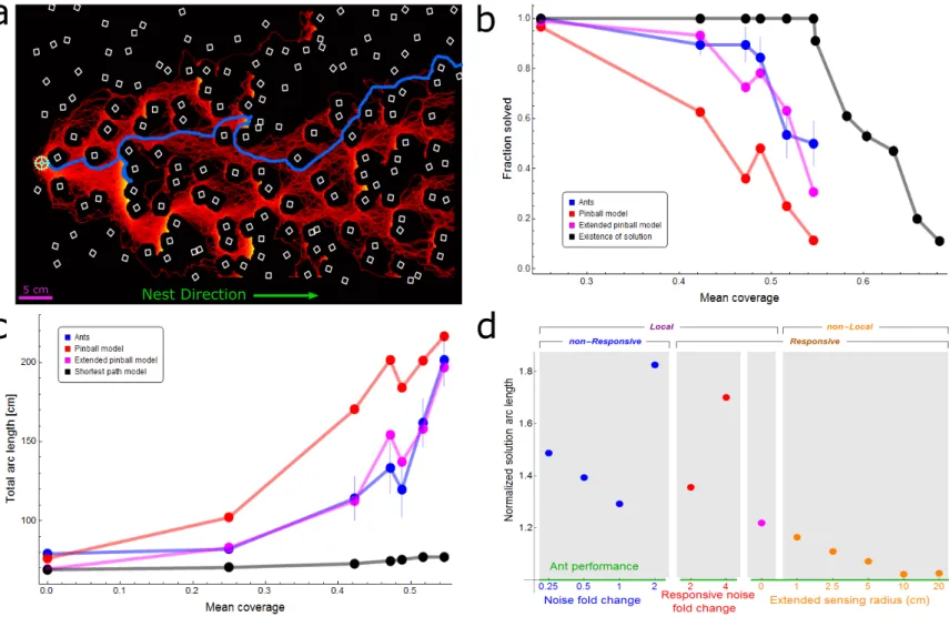
footage (200 instantiations per cube configuration, see trajectory heat map example in figure 2a). As expected,
94
increased cube coverage renders the simulation less effective in terms of success probability, solution times and
95
total trajectory arc length (figure 2b-c, Appendix 2-figure 2b).
96
We go on to compare the performance of the pinball model to that exhibited by the ants (figure 2b-d). By
97
construction, in the absence of cubes the pinball model performs similarly to the ants. This similarity carries
98
over to low density mazes, which were mostly composed of isolated cubes, since both the ants and the pinball
99
simulation quickly roll across these small obstacles. At intermediate cube densities, where composite obstacles
100
are present, the ants outperform the physical model by a gap that widens with increasing cube number. Finally,
101
both algorithms are similarly ineffective at solving very dense mazes. The ants’ performance surpasses not
102
only that of the pinball model but also variants of this model with other noise statistics (see figure 2d - blue
103
points/axis, Appendix 2.1,2.2 and Appendix 2-figures 1,2). Figure 2d summarizes the comparisons between
104
empirical ant performances and those of different numerical simulations and is referred to below as further
105
models are introduced.
106
Collective extension of sensing range
107
Percolation mazes can be viewed as a collection of disjoint traps [24] (figure 3b). Therefore, to identify
108
the crucial ingredients which help the ants outperform local physical models we focused on motion within such
109
traps. Much like local maxima in optimization problems, traps are areas in which motion towards the global
110
solution is blocked. Escape from a trap must therefore be facilitated by secondary forces that are not aligned
111
with the general bias. Similar to common optimization heuristics [35], in the pinball model these forces are the
112
result of random noise. The ants, however, exhibit more elaborate motion. We find that when the carrying
113
group enters a trap, its characteristics of motion change; specifically, they spend a higher percentage of the time
114
walking against the bias (Appendix 1.4, Appendix 1-figure 2).
115
It was previously shown for ants [36], [37] (and other animal groups [38], [39]) that physical interaction with
116
a trap can induce change in the collective characteristics of motion. This responsiveness does not require any
117
individual to be explicitly aware of the trap and can therefore be perceived as implicit, emergent trap detection.
118
However, our simulations show that mere responsiveness to local information does not suffice in explaining the
119
ants’ enhanced performance (see local responsive algorithms in figure 2d, Appendix 2.2,2.3, Appendix 2-figures
120
2c,3).
121
Beyond the effect of local mechanical collisions, the collective motion of P. longicornis is known to be
122
guided by information that is brought in by newly attached transient leader ants [14], [37]. Once attached,
123
these ants steer the entire group and determine the collective direction of motion. Leader ants come from the
124
non-carrying population which surrounds the load [14], [31]. Their attachment therefore allows carrying ants to
125
use information that is beyond the load’s immediate locality and could enable the group to collectively extended
126
their sensing range [29]. Next, we estimate the distance at which information is gathered and assess the impact
127
of this form of non-locality on global performances.
128
To approximate the sensing radius, we focused on the spatial distribution of non-carrying ants around a
129
trapped load (figure 3a, Materials and Methods). We find that when the load is delayed within a trap,
non-130
carrying ants spread across a circular region whose outer radius, rantssense, is on the order of 10cm (figure 3a, figure
131
3 supplement 2) . Although a relatively small fraction of the ants reach areas that are rants
sense centimeters away
132
from the load, this is the relevant length scale to consider; this is since even a single leader ant suffices to steer
133
the entire group and guide it as far as 10cm [14]. Hence, when the load is delayed within an obstacle, leader
134
ants constantly present the carrying group with potential crossing routes up to a 10cm radius. Collectively,
135
this implies that a number of potential routes are presented in parallel to the carrying group. In turn, the
136
coordinated motion allows the group to explore the suggested traversal routes [37] until, eventually, they find
137
d
a
Nest Direction 5 cmc
b
Figure 2: Ant vs. simulation performances. (a) Heat map of trajectories of 200 simulation iterations over an example maze (brighter colors signify more visits, cubes are drawn in white). Actual ant trajectory for this maze is overlaid in blue. Initial location for all trajectories is marked by a green cogwheel. (b) Probabilities to solve the maze as a function of mean coverage, for ants (blue), pinball model (red), and extended pinball model (magenta) simulations. The percent of solvable mazes is depicted in black (up to 0.55 coverage - experimental mazes, 0.55 coverage and above - computer generated mazes). Sample sizes (from small coverage to large): Ants - 15,57,19,19,28,30, Pinball Model - 200 iterations each over 10,14,10,8,15,11 distinct mazes, Extended Pinball Model - 500 iterations each over 10,14,10,8,15,11 distinct mazes. Existence of Solution - (experimental - up to 0.55 coverage): 10, 14, 10, 8, 15, 11 (generated- 0.55 coverage and beyond): 100 for each coverage. (c) Comparison of average total arc length of ants’ and different types of simulations’ trajectories (color scheme as in (b)). The geodesic shortest path traversing the maze is shown in black. We take into account the different success rates of the simulation and ants as shown in panel (b) by adding a penalty to each iteration/experiment which was not successful. The added penalty equals average speed multiplied by the time stuck before termination of experiment/iteration. Error margins in (b,c) are standard errors of the mean. Wherever no error is visible, the error is small enough to fit within the filled circle marker. Sample sizes (from small coverage to large): Ants - 31,10,14,10,8,15,11, Simulations - as in (b) except the first point is 200/500 iterations in the no cubes case, Shortest Path - 10,14,10,8,15,11, first point is simply the width of the board. (d) The performance of different simulated models normalized by empirical ant performance. We use a single inverse measure for the performance of the simulations: Lsim
Lants, where L is the solution arc length (calculated as in panel (c)) averaged over all cube densities. Models are categorized by their locality and responsiveness, and separated into three differently colored x-axes; each corresponding to a different kind of simulation, wherein the numeric value is the main parameter we change in that simulation. Local non-responsive models are versions of the pinball model where noise levels were varied (Blue dots over blue axis, a noise value of 1 is the fitted value in original model. Appendix 2.1 and Appendix 2-figure 1). Local responsive models are versions of the pinball model in which noise is temporarily altered in response to the load being stuck in a trap (Red dots over red axis, Appendix 2.3 and Appendix 2-figure 3) or a new random bias direction is temporarily selected (Magenta dot over orange axis, Appendix 2.2 and Appendix 2-figure 2). The non-local responsive models are versions of the extended pinball model with different sensing radii (Orange dots over orange axis, Materials and Methods, Appendix 2.4, Appendix 2-figure 4). For
an escape route that bypasses the obstacle [31]. Indeed, we find that preventing ants from entering the trap
138
from detour routes significantly reduced the extent of the ants’ collective exploration (see Appendix 1.7 and
139
Appendix 1-figure 4).
140
Extended sensing facilitates efficient trap and labyrinth traversal
141
To assess the contribution of the extended sensing to trap negotiation, we considered an extended-pinball
142
model with an enlarged sensing range, rsense(see Materials and Methods). This is a responsive model in which
143
obstacle sensing induces temporary change in the direction of the bias. Unlike the responsive local models
144
described above (figure 2d), in the extended pinball model the choice of the temporary directional bias is
145
affected by non-local environmental structure. Specifically, the direction of this temporary bias was chosen to
146
lead towards a point along the obstacle’s boundary that is conducive to bypassing the obstacle, entails minimal
147
directional changes ([14], [40]), and is no further than a distance of rsensefrom the load’s center (for more details
148
see Materials and Methods). We ran computer simulations of this model over the experimentally acquired cube
149
maze configurations - 500 instantiations per cube configuration.
150
Next, we compared the effectiveness of trap escape by the ants, the pinball model and the extended pinball
151
model. To do so, we defined the depth of a trap as the length of the geodesic required to escape it (Appendix 1.5
152
and Appendix 1-figure 3). We then quantified how well the ants and the simulations perform when facing traps
153
of a given depth independent of the overall complexity of the maze. This was done by assessing the average
154
distance travelled to escape the trap, normalized by trap depth. In the basic pinball model, this ratio increases
155
with trap size as would be expected from a random walker that relies on rare large fluctuations to escape. The
156
ants do much better: up to trap depths that roughly coincide with the measured upper bound on their sensation
157
range, namely rants
sense, the ants’ escape route is highly efficient, i.e. it scales linearly with trap depth (see [31]).
158
For traps that are deeper than rants
sense the ratio quickly rises. The extended pinball model highlights the role
159
that sensing range plays in trap escape. To efficiently bypass a trap of a given size the sensing range must be at
160
least as large (see Appendix 2-figure 4c). Specifically, setting this sensing range to its experimentally measured
161
upper bound rsense= rantssense yields trap solution performance similar to that of the ants (figure 3c-d).
162
We now turn to check how non-local information and the resulting improvement in negotiating
medium-163
sized traps (i.e. up to rants
sense) reflect on overall performance. We find that the extended pinball model simulations
164
with rsense = rantssense performed significantly better than the original pinball model and almost matched that
165
of the ants (see figure 2b-c). In addition, we found that simulating the extended pinball model with values of
166
rsense that are smaller than rsenseants diminished performance. Conversely, increasing the value of rsense beyond
167
rants
sense had no effect on overall performance (see figure 2d - orange points/axis, Appendix 2.4 and Appendix
168
2-figure 4a,b).
169
We note that while the performances of the extended pinball model with a sensing radius of rants sense are
170
comparable to those of the ants, they are still slightly inferior (figure 2b-c). This may be expected due to the
171
relative simplicity of this model which does not aim to precisely replicate the distributed nature and navigational
172
capabilities of ants. Rather, this model is intended to capture the ants’ extended sensing range and demonstrate
173
d
c
a
5 cmb
5 cmFigure 3: Simulation and ant performance near traps. (a) Logarithmic heat map showing the spread of ants while the load is located near the top of a deep triangular trap (extracted from 23 minutes of footage). Color intensity represents the total number of ant counts within each 2D bin over the aforementioned experimental duration. A rants
sense ∼= 10 cm
radius area centered on the load contains ∼99% of ant traffic in the vicinity of the load (see figure 3 supplement 2).
Inset shows an example image from the video footage of the experiment. (b) Illustration of traps on a sample maze. Each group of cubes comprising a trap are connected by gray lines and colored according to the trap depth in cm (as defined in Appendix 1.5) corresponding to the color bar. The empirical ant trajectory for this particular realization is plotted in blue (initial location marked using a pale green cogwheel). (c) Probability of trap solution as a function of trap depth for ants (blue), pinball model (red), and extended pinball model (magenta). Sample sizes (from shallow trap to deep): Ants - 73,70,35,22,19,6,3, Pinball Model - 2645,2886,1646,1289,982,343,105, Extended Pinball Model - 8979,8203,4637,3395,2042,815,403. (d) Average normalized arc length of the trajectory taken to solve a trap as a function of trap depth for ants and simulations (color scheme as in (c)). Trajectory lengths are normalized by trap depth (see Appendix 1.5, Materials and Methods) Ant performance is approximately constant up to D = 12 cm which is on the scale of rants
sense(see panel (a)). Sample sizes: Ants - 73,70,35,21,14,4,1, Pinball Model - 2620,2675,1352,530,136,60,0,
Extended Pinball Model - 8952,7969,4497,3347,1913,620,302. Error margins in (c,d) are standard errors of the mean. Wherever no error is visible, the error is small enough to fit within the filled circle marker.
the navigational importance of collecting information beyond the physical boundaries of the load.
174
The relation between the ability to escape a single disjoint trap and overall performance in crossing the
175
entire terrain relies on the statistics of trap sizes in the environment. Indeed, we find that below the ants’ solution
176
threshold of 55% coverage, close to the system’s actual percolation threshold, the vast majority (93.6%) of the
177
traps are smaller than rantssense (figure 4a, Appendix 1.6, figure 3 supplement 1). The ants’ efficient performance
178
at the global level can therefore be traced to their ability to quickly overcome traps up to this size. Moreover,
179
the rarity of large traps renders larger sensing ranges unnecessary. Next, we present theoretical analysis to make
180
these intuitive points more precise.
181
Logarithmic sensing radius suffices to approximate the shortest path
182
Percolation theory deals with statistics of cluster sizes on random graphs while the Ant-in-a-Labyrinth
183
literature examines motion over such graphs. These fields of study could therefore provide firm theoretical
184
grounds for studying the relations between environmental statistics and collective navigation as found in our
185
experiments.
186
A main result of the ant-in-a-labyrinth literature is that a pure random walker would cross the percolation
187
maze in a time that scales quadratically with the size of the system [26]. Moreover, adding a small bias to the
188
random walk results in much faster passage times that are linear in system size [24], [41]. Further increasing
189
the bias does not necessarily increase speed since the walker tends to get trapped. This implies the existence
190
of an intermediate bias in which traversal speed is maximized [42]–[44] - we verified this theoretical result by
191
simulation (figure 4b). In all these cases, the sensing range of the walker is, by definition, zero. It is therefore
192
interesting to compare these performances to those of an ant-inspired random walker with an extended sensing
193
range.
194
Our main theoretical result concerns the impact of moderately extending the sensing range [45] to be
195
logarithmic in system size. We first used simulations to show that such a modest extension can lead to a huge
196
(over 200-fold) speed up in traversal times when compared to classical ant-in-a-labyrinth solutions (figure 4b,
197
Appendix 3.2). Then, to better understand the origin of this result, we combined mathematical analysis and
198
simulation (figure 4c) to show that a walker whose sensing range is logarithmic in system size can cross the
199
labyrinth along a path that approximates the shortest possible path to extremely high precision (Appendix
200
3.1,3.2, Materials and Methods, Appendix 3-figure 4a).
201
We next present an outline of the formal arguments laid in detail in Appendix 3. Our analysis can be
202
broken into three parts: First,we prove that two distant points on a percolation grid above the percolation
203
threshold (p=0.5) can be connected along a path that is fully confined to a narrow strip (figure 4c). Second,
204
we use numerical calculations to show that the length of this confined path is extremely close to the length of
205
the shortest possible path between these two points. Finally, we provide an algorithm for a mobile agent with a
206
logarithmic sensing range which allows the agent to proceed along a path that is extremely close to the confined
207
path and, therefore, to the shortest possible path between the two points.
208
More specifically, we considered a percolated grid above the percolation threshold, and two points s and t
209
that belong to the infinite connected component. For the first aforementioned part, we aim to prove that with
210
high probability there exists a path that connects these two points and is completely contained in a strip S of
211
logarithmic width around the aerial line that connects the two points (colored gray in figure 4c). Essentially, this
212
result follows from a result by Aizenman and Newman [46] which states that, above the percolation threshold,
213
the probability of obtaining an obstacle decreases exponentially with its size. This implies that if the aerial
214
distance between the points is d, then with high probability, there will not be an obstacle larger than W = c log d,
215
for some constant c > 0, which blocks the aerial line between them. Taking the width of the strip S to be
216
slightly larger than W , ensures that, with high probability, there is a path which is contained in S and bypasses
217
these obstacles. Having established the existence of such a path, we denote the length of the shortest of all such
218
paths by ˜D.
219
Next, we numerically demonstrated that ˜D is extremely close to D, the unrestricted shortest path between
220
s and t (figure 4b). This was done by first generating random lattices slightly above the percolation threshold
221
(p=0.55). We then define a narrow strip within it and calculate the shortest path, where the path is either
222
unconstrained and can include any vertex on the entire lattice (D) or constrained to stay on the strip ( ˜D).
223
These shortest paths were calculated by finding the regional minimum of the summation of two geodesic distance
224
transforms over image representations of the random lattice, with the two edges of the strips acting as seed
225
locations. To get the shortest path constrained to the strip, we simply ran the same calculation on the subset
226
of the maze which only contains the strip. We find that the average percent of increase to the length of the
227
shortest path when constrained to the aforementioned strip is merely∼0.46% (for d = 70000).
228
Finding a path whose length approximates ˜D may not be a trivial task for an agent with a small
vision-229
radius. As our main theoretical result, we prove that a logarithmic field of view, r = b log d, suffices to yield
230
paths that closely approximate the length of ˜D. In fact, by appropriately choosing the constant b we can
231
guarantee that the length of the resulting path will approximate ˜D to any desired approximation. To achieve
232
this, the agent executes a series of short bouts where each allows it to reduce its aerial distance to t by roughly
233
log d (figure 4c). At the beginning of a bout the agent assesses all paths that start at its current location (node
234
u in figure 4c), are contained within its sensing range, r (black square in figure 4c), and lead to some point v, in
235
the strip S (colored gray in figure 4c) which is roughly log d closer to the destination (node v in the “goal set”
236
in figure 4c). It then advances along the shortest of these paths (which exists with high probability). Since the
237
bout starts and ends in S, any deviation from S stays within the radius r, and is hence small (figure 4c). Since
238
the sensing radius, r, is larger than the width of the strip, the trajectory chosen by the agent can be shown
239
to be extremely close to the shortest path that is fully contained in the strip and advances the same distance.
240
Stringing these bouts allows the agent to cross the maze on a path whose length is extremely close to ˜D and,
241
in turn, to the shortest possible distance D.
242
Relating theoretical results and empirical findings
243
The theorem outlined above shows that a small logarithmic sensing range suffices for fast traversal of a
244
percolation maze. The theoretical results further indicate that a route that is confined within a narrow strip
245
s
t
sensing radiusu
goal setv
a
b
c
Optimal BiasFigure 4: Efficiency of logarithmic range extended sensing. (a) The fraction of cubes which belong to dif-ficult traps, out of the total number of cubes in the system, as a function of mean coverage of the cube maze. Difficult traps are those defined by D > rants
sense. Note the sharp increasing trend above 0.55% coverage. Error
margins are standard errors of the mean. Sample Sizes (from small coverage to large): Experimental (number of cubes in the calculation) - 1017,2511,2033,1631,3380,2798, Generated - 50 different mazes for each cube number: 100,200,225,250,275,300,325,350,400,425,450. (b) Simulated performances of percolation lattice solution algorithms just above the percolation threshold (p = 0.55). The biased random walk model whose bias, B = 0.045, is optimized [24] to increase drift speed (see inset) performs significantly worse than a simulated logarithmic extended sensing algorithm. The extended sensing algorithm is only slightly worse than the overall shortest path and the shortest path that is constrained within a logarithmic width strip crossing the maze. Error bars in the main panel and shaded regions in the inset signify standard deviation. Sample sizes: Main figure - calculation for the first 3 bars is one number per maze. The last bar is a simulation with 200 iterations over each maze. Since we used 50 different lattice configurations, the sample size is 50,50,50,10000. Inset - 200 iterations over 50 different lattices; thus, 10000 samples per point. (c) Schematic illustration of the theoretical extended-sensing algorithm on a 2D percolation grid (see Materials and Methods, Appendix 3.1,3.2). Red lines are the open edges of the infinite cluster across which the walker moves from an initial point s to a final point t. The walker moves by executing a series of short bouts. Depicted in the image is a single bout wherein the agent, currently positioned at point u, accesses information within its sensing range (black square, of logarithmic radius) and advances along the green geodesic (fully contained within the sensing range) to some point v on the next goal set line. Such bouts allow the agent to cross the maze on a path whose distance is extremely close to that of the shortest path (blue line) between the initial point s and the final point t, that is contained within a strip of logarithmic width (colored
around the aerial line connecting the start and end points can well-approximate the shortest path possible. In
246
other words, the proof and accompanying simulations suggest that efficient labyrinth crossings do not require
247
significant deviations from the aerial line. In line with this suggestion, we find that the empirical load trajectories
248
are typically confined to relatively narrow strips, even at high cube densities (figure 4 supplement 1).
249
To further interpret our experimental results in light of our theory, we must first return to their underlying
250
assumptions. While in our experiments we vary the density of open edges p, in our theoretical results we
251
assume a fixed value p0 which is above the percolation threshold. To reconcile these analyses, we note that for
252
a sufficiently large system size, N , the dominant factor in the sensing range required to solve the maze would
253
be log N . This logarithmic sensing range then suffices for the entire range of mazes with p ≥ p0, i.e., mazes of
254
the same size whose coverage is lower.
255
Our theoretical analysis thus predicts a logarithmic relation between system size and sensing range. An
256
algorithm implementing this sensing range can efficiently navigate most solvable mazes of the corresponding
257
size. We next turn to apply this result to quantitatively relate two empirical length scales: the size of the ants’
258
foraging range which, in the case of this species, is on the order of 10 meters [47], and the scale of extended
259
sensing which is on the order of 10 cm. To make this relation, we must specify a third length scale - the
260
spacing of the abstract grid used in our proofs. We note that grid spacing coincides with the length of a cube’s
261
edge which is 1 centimeter. Indeed, the addition of a single cube translates to the removal of an edge in the
262
percolation grid. We further note that both cube size and experimental load radius are not arbitrary. They
263
were both chosen to coincide with the typical size of the loads cooperatively transported by longhorn crazy
264
ants [14], [16]. Smaller obstacles will not stall the carrying group. Larger, extended obstacles can no longer be
265
approximated by a percolation network.
266
With these numbers in hand we can now verify whether the ants’ natural sensing range is congruent with
267
our theoretical results. Given the 1 centimeter grid spacing, a foraging range of 10 meters coincides with a
268
system size of N = 1000. According to our theoretical results, the expected sensing range at this system size
269
is on the order of log(1000) ≈ 10. Translating the answer back into centimeters, we find that the ants’ sensing
270
range is expected to be on the order of 10 centimeters. This length scale coincides with our empirical findings
271
regarding both the ants’ sensing range and the strip width to which their collective solutions are confined (figure
272
4 supplement 1).
273
We wish to stress that these measures are not meant to be precise. First, our experimental system’s length
274
is 70 centimeters, which is substantially smaller than the ants’ maximal foraging range. This is not a major
275
concern since optimal sensing ranges are robust across system sizes due to their logarithmic nature. The optimal
276
sensing range for a 70 centimeter system is only log(1000)/ log(70) = 1.6 times smaller than the sensing range
277
that corresponds to a 10 meter foraging range, and is still on the order of 10 centimeters. Second, there is no
278
reason to believe that the ants are optimally tuned for the environments studied in this paper or for a specific
279
system size. We merely claim that the sensing range we measured is extremely efficient for traversing disordered
280
systems of varied sizes and densities. It is this kind of generality one might expect from natural navigational
281
systems that must deal with a large number of unexpected challenges.
282
Discussion
283
An organism’s survival depends on its ability to overcome challenges towards reward. The evolution of
284
such abilities can be affected by various factors including the difficulty of the challenge, its prevalence [48], the
285
reward it entails [49] and the energetic cost of maintaining cognitive and physical capabilities required to tackle
286
it [50]. Accommodating these possibly conflicting considerations can lead to evolutionary trade-offs in problem
287
solving abilities [51]–[54]. The navigation behavior we describe may be the result of such a trade-off: the ants
288
use their distributed nature to probe the surroundings non-locally but only moderately extend their sensing
289
range. The extreme navigational efficiency induced by this moderate increase in sensing range stems from the
290
fact that it matches the statistics of trap sizes in percolation networks. Indeed, percolative environments, either
291
below or above the percolation threshold, hardly exhibit any traps of intermediate size [20] and navigational
292
strategies to tackle such traps are thus useless.
293
The ants use remote, active, collective sensing to probe their surroundings. Remote sensing is extremely
294
common in the biological world [55]. Primary examples are the use of sight, olfaction, hearing, and vibration
295
[56], [57]. Animal remote sensing also extends to the use of more active tactics such as echolocation [58] and
296
active electrolocation [59]. Most ant species are known to use eyesight to assist their navigation [60]. However,
297
since ants are physically small in comparison to the smoothness of the surfaces they inhabit, their lines of
298
sight along these surfaces are inevitably short. Thus, sight does not suffice to bypass local obstacles during
299
cooperative transport. Instead, the ants use their numbers to actively extend their sensing range by sending
300
out scouts in all directions. Indeed, evolutionary trade-offs as discussed above can be expected to be prevalent
301
in cases of active sensing [61].
302
This brings us to the second aspect of the ants’ extended sensing; namely, the fact that it is collective.
303
It is not uncommon that animal groups engage in collective sensing. For example, the “many eyes principle”
304
describes the ability of a group of prey animals to share surveillance efforts, such that the first to spot an
305
approaching predator can warn the rest [62]. Another striking example comes from fish shoals; golden shiners
306
use collective sensing to track environmental features that are unavailable to individuals and only make sense
307
on the scale of the group [29]. This collective effect is reminiscent of the ants’ collaborative navigation scheme
308
studied here. Indeed, as a group, the ants manage to find navigational solutions to large obstacles that are
309
imperceptible to any single individual [31].
310
The ‘ant-in-a-labyrinth’ problem was originally suggested by Pierre De-Gennes as a means of investigating
311
diffusion through disordered media [21]. It applies, for example, to the motion of an electron in a metal-insulator
312
alloys under an electric field and at some finite temperature [63]–[65]. The electron can be modeled as a random
313
walker on a percolation network where the effect of the electric field is captured by a drift term and the effect of
314
temperature by an additional random component. This biased random walk framework underlies most
ant-in-315
a-labyrinth literature [19]–[27]. Inspired by the ants’ behavior, we took a more algorithmic perspective to this
316
problem. Instead of studying the properties of a walker with a given set of local rules fixed by the laws of physics,
317
we explored the impact of extending the sensing range on navigational performances. Such studies regarding the
318
effects of locality on performances are, in fact, a common theme in theoretical computer science [66]. In general,
319
local algorithms are often preferred for their simplicity. However, it is known that they can fall short under
320
different circumstances [66]–[70]. Indeed, we have seen that in our system the performance of physics-based
321
local algorithms is substantially inferior to the ants’ performance. Conversely, extending the sensing range to
322
be logarithmic in the size of the grid can have a significant impact on navigation time, overshadowing purely
323
local solutions [31], [35], [71].
324
Finally, the wide applicability of percolation theory leads us to hypothesize that similar relations between
325
environmental structure and perception range may carry over to other biological systems. These include
popu-326
lations that occupy an extended area in either physical [29], [72], [73] or abstract [74] space. Spreading allows
327
the population as a whole to sample the space in a non-local manner. As an example, robustness and neutral
328
mutations allow an evolving population to spread over areas in fitness space. This non-locality enables
paral-329
lel sampling of the fitness landscape and increases the ability of the population to incorporate advantageous
330
mutations [74].
331
Supplement captions (figures, movie, and data sets)
332
1. Figure supplement to figure 1 (1) caption: Fraction of forbidden space and dense maze solving
333
probabilities. (a) The fraction of space blocked by obstacles (mean coverage), as a function of number of
334
cubes for computer-generated mazes (red) and experimental configurations (blue). Namely, the space the
335
center of the R = 1 cm ring-shaped load cannot reach. Mazes of the maximum density the ants were able
336
to solve (300 cubes) are already at an impressive 55% coverage. Shaded regions correspond to standard
337
error of the mean. Wherever no error is visible, the error is small enough to fit within the filled circle
338
marker. (b) The fraction of solvable computer-generated dense cube mazes as a function of mean cube
339
coverage is monotonically decreasing, as expected. Mazes with coverage greater than 0.62 (corresponds
340
to 400 cubes roughly) are unsolvable more often than not, with the greatest density mazes being solvable
341
only∼10% of the time.
342
2. Figure supplement to figure 3 (1) caption: Trap depth distributions. Bee swarm plot displaying
343
distributions of trap sizes as a function of mean coverage. Medians and means are represented by green
344
rectangles and red pluses, respectively. The data is taken from experiments for coverage <= 0.55 (blue),
345
and from computer generated mazes for coverage >= 0.55 (orange). Solid black horizontal line represents
346
the ants’ sensing radius rantssense= 10. Dashed black vertical line represents the maximal maze coverage the
347
ants solved. Dashed gray line represents the percolation threshold of the system. Note that unsolvable
348
traps were not included in the plot. For this reason there is less data displayed for the very high coverage
349
distributions.
350
3. Figure supplement to figure 3 (2) caption: Cumulative ant spread. Cumulative percentage of recognized
351
ant counts as a function of distance from the center of the load (when it is located at the apex of the trap)
352
in centimeters. The distribution reaches 99% at a distance of ∼14.1 cm (red dashed line), which is on the
353
order of 10 cm.
354
4. Figure supplement to figure 4 (1) caption: Carried loads stay within a confined strip. 90thpercentile
355
of perpendicular distance from mean direction of motion of the cooperatively carried load as a function
356
of mean coverage, for all obtained load trajectories. We see that the ant group stays within a distance of
357
∼4-6 cm from the mean direction of motion. As expected, this distance grows slightly with mean coverage,
358
since the path naturally must be more winding. Shaded area is the standard deviation.
359
5. Movie 1 caption: An example of cooperative transport of a 1 cm radius ring-shaped load across a 260
360
cubes maze. The nest is located to the right. The video is sped up X8 of real-life speed.
361
6. Source data 1 - cube locations data set caption: Coordinates of vertices of cube bases, specified in cm,
362
relative to a known (0,0) point marked on the experimental board. Each row in every file corresponds to
363
the four vertices of a single cube, ordered as follows: X1, Y1, X2, Y2, X3, Y3, Y4.
364
7. Source data 2 - load trajectory data set caption: Experimental load trajectories, specified in cm, relative
365
to a known (0,0) point marked on the experimental board. Format is X,Y coordinates as a function of
366
time. Time interval between samples is 0.04 seconds, except for videos 1440005 and 1440011, where the
367
time interval is 0.02 seconds.
368
Materials and Methods
369
Experimental setup: percolation experiment
370
Data was collected from 2 nests of Paratrechina longicornis in the Weizmann Institute of Science area,
371
Rehovot, Israel. Tests were carried out during the summer when these ants display collective transport behavior
372
[75]. Experiments were conducted on a 70x50 cm board on which ants were allowed to cooperatively carry heavy
373
loads. In each nest site, the testing board was positioned according to the availability of appropriate filming
374
conditions (flat floor and a sufficiently large area with uniform illumination). As P. longicornis are a polydomous
375
species, a 3-sided plastic frame was place around the board, with the opening directed towards the largest nest
376
entrance. This was done to make sure the bias the ants exhibit is directed towards the same nest direction, i.e.
377
there are no conflicting biases.
378
Before each experiment, a specific amount of cubes were randomly spread over the board. Ants were then
379
recruited using Royal CaninTM cat food. The cat food morsels were gently picked up and moved backwards
380
several times until a clear trail was established to the initial load location near (x, y) = (0, 25) on the board.
381
The cat food morsels were then removed and instead the ants were given an artificial ring-shaped 1.5 mm thick,
382
1 cm radius silicon load. The artificial objects were stored in advance overnight in a closed bag of cat food from
383
the same brand, to make them attractive to the ants. The board and load were marked with different colors to
384
facilitate image analysis and tracking.
385
After recruitment and positioning of the load at the initial location, the carrying process through the cube
386
maze was allowed to unfold without intervention. The entire process was recorded using a Panasonic HC-VX870
387
camcorder at a 4k resolution with a frame rate of 25 frames per second in most cases (a small fraction of the
388
experiments were recorded at HD resolution with a frame rate of 50 frames per second).
389
Experiments were declared to be over if one of three conditions was fulfilled:
390
1. The ants were able to solve the maze; i.e., the load exited the board through the edge close to the nest.
391
2. After a minimum of 8 minutes of experiment, if the ants were not able to solve the maze.
392
3. The ants were able to overcome the cubes by climbing over them with the load. As this behavior was
393
displayed only when the load was very much stuck, these experiments were considered as unsuccessful
394
trials (i.e. - the ants were considered unable to solve the maze).
395
Each maze was tested once, before repeating the process of maze creation, recruitment and carrying.
396
Experimental setup: wedge experiment
397
Unsolvable wedge-trap experiments were performed to assess the spatial distribution of non-carrying ants
398
around the load while it is trapped. These experiments were conducted on a single colony within the Weizmann
399
Institute of Science, Rehovot, Israel. Here, the board was a blank A3 page which was put within a dedicated
400
elevated perspex arena open on one side, with a paper ramp connected to it. The open side was directed towards
401
the nest entrance. Two different set-ups were tested: a wedge-shaped unsolvable trap was created either by
402
manually setting cubes∼1.5-2 cm apart (a composite trap), or by appropriately positioning two perspex plates
403
(a single entrance trap). Only the entrance in the latter set of experiments was also composed of cubes, to
404
produce the same difficulty in the front of the trap. The ants were recruited using a procedure similar to the
405
one used for the percolation experiment (see above section), and then allowed to carry the load for extended
406
periods of time (i.e. hours). These experiments were recorded using a Panasonic HC-VX870 camcorder at HD
407
resolution with a frame rate of 50 frames per second.
408
Image processing
409
Videos were analyzed using custom code built in MATLAB. One program was dedicated to tracking the
410
motion of the center as well as the orientation of the load, based on iterative HSV thresholding of the image
411
to recognize the colored markings on the load. Ants carrying the load were also recognized by transforming
412
the image into grayscale and performing homomorphic filtering before applying a threshold. Ant blobs were
413
distinguished from other blobs based on features such as circularity and eccentricity.
414
Cube locations were recognized by another specialized program, through a combination of HSV and RGB
415
thresholding. Cube blobs were automatically recognized and subsequently manually corrected using a GUI.
416
Cube base locations were then extrapolated from the obtained cube blobs.
417
The original video had a small effect of pincushion distortion which was accounted for using a spatial
418
distortion fixing transform. Load trajectories and cube locations were corrected.
419
Calculation of trajectory arc length of single trap solutions
420
In figure 3d we show the mean arc length obtained for crossing single traps of different depths. To calculate
421
this value, we considered the relevant trajectory section to begin when the ant team/simulation reaches a point
422
1 cm away from a trap, and ends when it advances 3.2 cm ahead in the nest direction (positive x direction),
423
thus assuring the trap is solved. This distance is in line with the distance used for trap definition (Appendix
424
1.5). The extra 3.2 cm is then deducted from the arc length. The arc length is then normalized by the trap
425 size, D. 426
Simulations
427 Physical Simulations 428All physical simulations were written based on CapSim[34], a MATLAB based physics engine aimed at
429
simulating multiple 2D rigid body mechanics. Based on our experimentally extracted cube locations, we used
430
CapSim to define the cubes and the edges of the board as collidable immovable objects. The load was defined
431
to be a disk of radius R = 1.1 cm, based on the experimental load size (R = 1 cm). The addition of 0.1 cm
432
is a result of evaluating simulation results allowing the load to pass through gaps the ants could not. This
433
correction compensates for inaccuracies in cube recognition due to image processing errors and difficulty in
434
assessing manually the cubes’ exact location due to their angle relative to the camera. At R = 1.1 cm there
435
was a strong correspondence between the ants’ and the simulated load’s ability to pass through gaps.
436
CapSim allows manipulating gravity g (analogous to the bias towards the nest), drag µ, and object mass m.
437
We also defined a random noise force term ν which is recalculated every time step and added to the gravity term.
438
The force direction is sampled from a uniform distribution, and its size is sampled from a normal distribution
439
with mean 0 and standard deviation σF. This parameter is important to simulate the inherent noise of the
440
biological system in question.
441
After fitting model parameters (see relevant section below), the simulation was run over all experimentally
442
implemented mazes (200/500 iterations each), allowing the dynamics to unfold up to a maximum time of Tmax.
443
Discrete biased random walk over continuous cube mazes
444
This simulation implements discrete biased random walk of a disc of radius R = 1.1 cm, moving across
445
the continuous cube mazes extracted from the experimental footage. The simulation was written in MATLAB.
446
The walker moves over the continuous board with a discrete step of size S = 0.1 cm. The direction of motion is
447
randomly assigned in every time step, where the probability of going towards the nest (to the right) is biased
448
such that pright= 0.25 + B and the other three directions are equally likely plef t = pup = pdown = 0.25 −B3,
449
where B is the bias parameter. At every time step, the simulation checks if the load’s suggested motion direction
450
leads to overlap with any of the cubes. If so, the direction is re-selected randomly; otherwise, the step is taken
451
in the selected direction. The edges of the board are treated as impassable walls.
452
After fitting model parameters (see relevant section below), the simulation was run over all experimentally
453
implemented mazes (100 iterations each), up to a maximum duration given by Tmax .
454
Simulations on discrete lattices
455
This set of simulations was developed to complement our mathematical proof regarding the efficiency of
456
the vision algorithm compared to biased random walk, on a dense percolation maze. To do so, we created
457
random percolation lattices poised just above the percolation threshold (which is 0.5 for bond percolation on
458
the Z2 lattice), p = 0.55. In line with the theoretical proof (Appendix 3.1), in these simulations, p is the
459
probability of an edge to be open or accessible. In all the simulations described in this section, the walker
460
moves over the giant component induced by the open edges of the lattice. 50 random lattices of dimensions
461
N Xδ log2(N ) = 70000X120 log2(70000) were generated. Following the theoretical considerations described in
462
Appendix 3.1, a concentric strip of width α log2(N ) = 20 log2(70000) (16 of the width of the lattice) was defined
463
as the ”internal strip”.
464
All simulations start at a node which is included in the giant component, closest to the center of the leftmost
465
column of the aforementioned internal strip. The goal of the simulations is to traverse the maze over the giant
466
component from this initial point to any point on the rightmost column of the internal strip.
467
As described in the main text, we ran two types of simulations. First, a simple biased random walker
468
simulation was run over all random lattice instances (50 iterations each), for different bias B values, where the
469
bias is defined as in the previous biased random walk simulations (see above). The second is an extended vision
470
algorithm. In this algorithm, the walker has a vision radius of γ log2(N ) = 20 log2(70000). Note that the vision
471
radius is equal to the width of the internal strip. At every time step of the simulation, the walker goes along the
472
shortest path within a square of edge size 2γ log2(N ), centered around its current location, ending at any point
473
which is both included in the giant component and contained within the column of the internal strip which is
474
located γ log2(N ) further in the positive x direction, measured from the current location (see Appendix 3-figure
475
3).
476
We also calculated for each lattice the overall shortest path (denoted D) and the shortest path fully
477
contained within the internal strip (denoted ˜D), from the leftmost column of the internal strip to its rightmost
478
column.
479
Fitting model parameters
480
Physical Simulations
481
Our system only has three free parameters since the drag term can be simply set to a constant and
482
incorporated into the other parameters of the system. We therefore set µ to a constant.
483
The other three free parameters were fit to global features of freely moving collective transport (i.e., no
484
obstacles) - mean trajectory arc length, mean velocity and two parameters describing the velocity-velocity cosine
485
correlation function. The parameter space was searched by running 30 iterations of the simulation without cubes
486
using 10 different values for each free parameter, totaling in 30000 iterations. The global features yielded by
487
the simulation were then subtracted from the experimental values and normalized to account for the different
488
scales of the parameter values. The parameters of the simulation yielding minimum error were then recognized.
489
This process was repeated 3 times, shrinking the searched parameter space to the distance between two points
490
of the prior computation.
491
The fitted values for the original simulation parameters are: µ = 10, g = −5.05, σF= 1277.8, m = 14.8571.
492
The simulation time step is ∆t = 0.04 seconds.
493
The low persistent noise variation of the simulation uses the following parameter values instead: σF= 250,
494
∆t = 0.4 seconds.
495
The simulation maximum duration Tmax = 8 minutes is equal to the experimental maximum allowed
496
duration.
497
Discrete biased random walk over continuous cube mazes
498
This simulation has two relevant parameters. The first - step size S, was taken to be 0.1 cm. The value of
499
the step size needed to be small enough to allow motion within traps and be compatible with the scale of the
500
cubes and the entire board. It also needs to be large enough to make the simulations fast enough, and allow
501
the simulation some chance to escape complex traps in reasonable time. We therefore took S = 0.1 cm to be of
502
the order of magnitude of the velocity of the ants.
503
The second parameter, the bias B, was fitted using global features of the motion of a freely carried load,
504
in a process similar to that described in the prior section. Here we used the mean deviation in the y-direction
505
and the mean trajectory arc length as the global features to fit. The obtained fitted value for the bias for our
506
simulation is B = 0.2211.
507
The simulation maximum duration Tmaxis derived from the average velocity of the ants along the trajectory
508
and the experimental maximum allowed duration. The result of the calculation was multiplied by five to give
509
the simulation greater chances of successfully navigating the cube mazes. The resulting value was Tmax= 7200
510
time steps.
511
Simulations on discrete lattices
512
We wanted to simulate the algorithm with the minimal vision radius such that the next destination column
513
would be fully visible from any point on the current column, thus α = γ. We also wanted to compare D with
514
˜
D in a non-trivial way and be able to increase the vision radius if needed, so δ > α and δ > γ. N was chosen
515
to accommodate computation power considerations. The maximum time allowed for the biased random walk
516
simulation was 150000 time steps. The maximum advancement in x for all biases after this running duration
517
made us realize there is no point in running the simulation until the maze is solved, and it is better to use a
518
speed measure obtained from the terminated walks.
519
Extended pinball model
520
The extended pinball simulations are the same as the original simulation except the addition of a module
521
responsible for alerting when the load is trapped, based on total motion in the x-direction in the last few seconds.
522
If the load moved less than ∆xmin in this period of time Tcompare, the load is considered to be stuck. When the
523
load changes its state from ”free” to ”stuck”, it acquires a new bias direction based on the local trap structure
524
(the algorithm calculating these directions is described below). Bias magnitude is constant and always set to
525
the parameter fitted to the ant behavior as explained above. The load then continues its motion in this altered
526
state for a duration Tchanged, after which it changes its state to ”free”, the bias vector reverts to its original
527
direction and it cannot become stuck again for another duration given by Tcooldown. This cooldown period is
528
added to make sure that if the load moved backwards it will not immediately switch back into the ”stuck” state.
529
The parameter values used for all extended pinball models (and temporarily altered noise) simulations
530
are: ∆xmin = 0.2 cm, Tcompare = 3 seconds, Tchanged = 4.48 seconds, Tcooldown = 4 seconds. The default
531
spatially extended sensing parameter used in the extended pinball simulations is rants
sense = 10. See Appendix
532
2.4 for the results of simulations with different rsense values. The extended pinball model further incorporates
533
time correlated Brownian noise to allow for more persistent motion towards escape. Importantly, correlated
534
Brownian noise alone did not lead to any improvement in global performance (see Appendix 2.2 and Appendix
535
2-figure 2).
536
The extended pinball simulations depend on the assignment of a new bias direction for the simulation
537
when the load becomes stuck. The assigned gravity direction is pre-calculated based on the local structure of
538
the obstacle hindering the load’s advancement. For each maze, we divided the space into 0.5X0.5 cm squares.
539
We then calculated the bias direction for each square center using the ”dilated cube” maze binary image (see
540
Appendix 1.5) and a spatially extended sensing parameter rsense. The following is a general outline of the
541
algorithm and does omit a few minor details dealing with certain edge cases:
542
1. Check if the square center falls within a blob. If it does not, continue the calculation using the square
543
center; otherwise:
544
(a) If the entire square is within the blob, ignore this square and continue to the next one.
545
(b) If the square contains part of the boundary of the blob, find the point on the boundary closest to
546
the square center. Continue the calculation using this point.
547
2. Check if there are any blob points in a straight line in the x-direction 0.25 cm in front of the point in
548
question. If not, then the load cannot get stuck in this square and therefore we can ignore this square and
549
continue to the next one.
550
3. Find the closest trap blob ahead of the point in question.
551
4. Find the point on the boundary of this trap closest to the point in question. We’ll refer to this point as
552
the seed boundary point.
553
5. Using this boundary point as a seed, calculate the geodesic distance in both directions (top and bottom)
554
over the boundary.
555
6. Cut two boundary pieces: from the seed boundary point to the point rsense cm away on the boundary in
556
the top direction. Do the same in the bottom direction.
557
7. For each boundary piece, find the point with the minimum x-value. We’ll refer to these as top and bottom
558
points.
559
8. Calculate the directions between the seed boundary point and the top and bottom points. Rotate by 15◦
560
to make the direction closer to that taken by an ant coming from the back. This is done because the
561
initially calculated directions often cross the trap blobs.
562
9. Select the new bias direction to be the one closer to the positive x-direction of the two options. This
563
is done to make sure the chosen direction is correct for small traps as well as traps which have an easy
564
solution in one direction. New calculated directions for large traps will point backwards in any case.
565
Acknowledgements
566
We would like to thank Yossi Yovel and Itay Benjamini. This work has received funding from the European
567
Research Council (ERC) under the European Union’s Horizon 2020 research and innovation program (grant
568
agreements No. 648032 and 770964). OF is the incumbent of the Henry J. Leir Professorial chair. EF is the
569
incumbent of the Tom Beck Research Fellow Chair.
570