HAL Id: hal-01240211
https://hal.archives-ouvertes.fr/hal-01240211
Submitted on 9 Dec 2015
HAL is a multi-disciplinary open access archive for the deposit and dissemination of sci-entific research documents, whether they are pub-lished or not. The documents may come from teaching and research institutions in France or abroad, or from public or private research centers.
L’archive ouverte pluridisciplinaire HAL, est destinée au dépôt et à la diffusion de documents scientifiques de niveau recherche, publiés ou non, émanant des établissements d’enseignement et de recherche français ou étrangers, des laboratoires publics ou privés.
Fast and compact self-stabilizing verification,
computation, and fault detection of an MST
Amos Korman, Shay Kutten, Toshimitsu Masuzawa
To cite this version:
Amos Korman, Shay Kutten, Toshimitsu Masuzawa. Fast and compact self-stabilizing verification, computation, and fault detection of an MST. Distributed Computing, Springer Verlag, 2015, 28 (4), �10.1007/s00446-015-0242-y�. �hal-01240211�
Fast and Compact Self-Stabilizing Verification, Computation,
and Fault Detection of an MST
Amos Korman∗ Shay Kutten† Toshimitsu Masuzawa‡
Abstract
This paper demonstrates the usefulness of distributed local verification of proofs, as a tool for the design of self-stabilizing algorithms. In particular, it introduces a somewhat generalized notion of distributed local proofs, and utilizes it for improving the time complexity significantly, while maintaining space optimality. As a result, we show that optimizing the memory size carries at most a small cost in terms of time, in the context of Minimum Spanning Tree (MST). That is, we present algorithms that are both time and space efficient for both constructing an MST and for verifying it. This involves several parts that may be considered contributions in themselves.
First, we generalize the notion of local proofs, trading off the time complexity for memory efficiency. This adds a dimension to the study of distributed local proofs, which has been gaining attention recently. Specifically, we design a (self-stabilizing) proof labeling scheme which is memory optimal (i.e., O(log n) bits per node), and whose time complexity is O(log2n) in synchronous networks, or O(∆ log3n) time in asynchronous ones, where ∆ is the maximum degree of nodes. This answers an open problem posed by Awerbuch and Varghese (FOCS 1991). We also show that Ω(log n) time is necessary, even in synchronous networks. Another property is that if f faults occurred, then, within the required detection time above, they are detected by some node in the O(f log n) locality of each of the faults.
Second, we show how to enhance a known transformer that makes input/output algorithms self-stabilizing. It now takes as input an efficient construction algorithm and an efficient self-stabilizing proof labeling scheme, and produces an efficient self-stabilizing algorithm. When used for MST, the transformer produces a memory optimal self-stabilizing algorithm, whose time complexity, namely, O(n), is significantly better even than that of previous algorithms. (The time complexity of previous MST algorithms that used Ω(log2n) memory bits per node was O(n2), and the time for optimal space algorithms was O(n|E|).) Inherited from our proof labelling scheme, our self-stabilising MST construction algorithm also has the following two properties: (1) if faults occur after the construction ended, then they are detected by some nodes within O(log2n) time in synchronous networks, or within O(∆ log3n) time in asynchronous ones, and (2) if f faults occurred, then, within the required detection time above, they are detected within the O(f log n) locality of each of the faults. We also show how to improve the above two properties, at the expense of some increase in the memory.
Keywords: Distributed network algorithms, Locality, Proof labels, Minimum spanning tree, Distributed property verification, Self-stabilization, Fast fault detection, Local fault detection.
∗
CNRS and Univ. Paris Diderot, Paris, 75013, France. E-mail: Amos.Korman@liafa.jussieu.fr. Supported in part by a France-Israel cooperation grant (“Mutli-Computing” project) from the France Ministry of Science and Israel Ministry of Science, by the ANR projects ALADDIN and PROSE, and by the INRIA project GANG.
†
Information Systems Group, Faculty of IE&M, The Technion, Haifa, 32000 Israel. E-mail: my last name at ie dot technion dot ac dot il. Supported in part by a France-Israel cooperation grant (“Mutli-Computing” project) from the France Ministry of Science and Israel Ministry of Science, by a grant from the Israel Science Foundation, and by the Technion funds for security research.
‡
Graduate School of Information Science and Technology, Osaka University, 1-5 Yamadaoka, Suita, Osaka, 565-0871, Japan. E-mail: masuzawa@ist.osaka-u.ac.jp. Supported in part by JSPS Grant-in-Aid for Scientific Research ((B)26280022).
1
Introduction
1.1 Motivation
In a non-distributed context, solving a problem is believed to be, sometimes, much harder than verifying it (e.g., for NP-Hard problems). Given a graph G and a subgraph H of G, a task introduced by Tarjan [65] is to check whether H is a Minimum Spanning Tree (MST) of G. This non-distributed verification seems to be just slightly easier than the non-distributed computation of an MST. In the distributed context, the given subgraph H is assumed to be represented distributively, such that each node stores pointers to (some of) its incident edges in H. The verification task consists of checking whether the collection of pointed edges indeed forms an MST, and if not, then it is required that at least one node raises an alarm. It was shown recently that such an MST verification task requires the same amount of time as the MST computation [26, 53]. On the other hand, assuming that each node can store some information, i.e., a label, that can be used for the verification, the time complexity of an MST verification can be as small as 1, when using labels of size Θ(log2n) bits per node [54, 55], where n denotes the number of nodes. To make such a proof labeling scheme a useful algorithmic tool, one needs to present a marker algorithm for computing those labels. One of the contributions of the current paper is a time and memory efficient marker algorithm.
Every decidable graph property (not just an MST) can be verified in a short time given large enough la-bels [55]. A second contribution of this paper is a generalization of such schemes to allow a reduction in the memory requirements, by trading off the locality (or the time). In the context of MST, yet another (third) con-tribution is a reduced space proof labeling scheme for MST. It uses just O(log n) bits of memory per node (asymptotically the same as the amount of bits needed for merely representing distributively the MST). This is below the lower bound of Ω(log2n) of [54]. The reason this is possible is that the verification time is increased to O(log2n) in synchronous networks and to O(∆ log3n) in asynchronous ones, where ∆ is the maximum degree of nodes. Another important property of the new scheme is that any fault is detected rather close to the node where it occurred. Interestingly, it turns out that a logarithmic time penalty for verification is unavoidable. That is, we show that Ω(log n) time for an MST verification scheme is necessary if the memory size is restricted to O(log n) bits, even in synchronous networks. (This, by the way, means that a verification with O(log n) bits, cannot be silent, in the sense of [33]; this is why they could not be of the kind introduced in [55]).
Given a long enough time, one can verify T by recomputing the MST. An open problem posed by Awerbuch and Varghese [15] is to find a synchronous MST verification algorithm whose time complexity is smaller than the MST computation time, yet with a small memory. This problem was introduced in [15] in the context of self-stabilization, where the verification algorithm is combined with a non-stabilizing construction protocol to produce a stabilizing protocol. Essentially, for such purposes, the verification algorithm repeatedly checks the output of the non-stabilizing construction protocol, and runs the construction algorithm again if a fault at some node is detected. Hence, the construction algorithm and the corresponding verification algorithm are assumed to be designed together. This, in turn, may significantly simplify the checking process, since the construction algorithm may produce output variables (labels) on which the verification algorithm can later rely. In this context, the above mentioned third contribution solves this open problem by showing an O(log2n) time penalty (in synchronous networks) when using optimal O(log n) memory size for the MST verification algorithm. In contrast, if we study MST construction instead of MST verification, time lower bounds which are polynomial in n for MST construction follow from [58, 62] (even for constant diameter graphs).
One known application of some methods of distributed verification is for general transformers that transform non-self-stabilizing algorithms to self-stabilizing ones. The fourth contribution of this paper is an adaptation of the transformer of [15] such that it can transform algorithms in our context. That is, while the transformer of [15] requires that the size of the network and its diameter are known, the adapted one allows networks of
unknown size and diameter. Also, here, the verification method is a proof labeling scheme whose verifier part is self-stabilizing. Based on the strength of the original transformer of [15] (and that of the companion paper [13] it uses), our adaptation yields a result that is rather useful even without plugging in the new verification scheme. This is demonstrated by plugging in the proof labeling schemes of [54, 55], yielding an algorithm which already improves the time of previous O(log2n) memory self-stabilizing MST construction algorithm [17], and also detects faults using 1 time and at distance at most f from each fault (if f faults occurred).
Finally, we obtain an optimal O(log n) memory size, O(n) time asynchronous self-stabilizing MST con-struction algorithm. The state of the art time bound for such optimal memory algorithms was O(n|E|) [18, 48]. In fact, our time bound improves significantly even the best time bound for algorithms using polylogarithmic memory, which was O(n2) [17].
Moreover, our self-stabilizing MST algorithm inherits two important properties from our verification scheme, which are: (1) the time it takes to detect faults is small: O(log2n) time in a synchronous network, or O(∆ log3n) in an asynchronous one; and (2) if some f faults occur, then each fault is detected within its O(f log n) neigh-bourhood. Intuitively, a short detection distance and a small detection time may be helpful for the design of local correction, for fault confinement, and for fault containment algorithms [43, 16]. Those notions were intro-duced to combat the phenomena of faults “spreading” and “contaminating” non-faulty nodes. For example, the infamous crash of the ARPANET (the predecessor of the Internet) was caused by a fault in a single node. This caused old updates to be adopted by other nodes, who then generated wrong updates affecting others [59]. This is an example of those non-faulty nodes being contaminated. The requirement of containment [43] is that such a contamination does not occur, or, at least, that it is contained in a small radius around the faults. The requirement of confinement [16] allows the contamination of a state of a node, as long as this contamination is not reflected in the output (or the externally visible actions) of the non-faulty nodes. Intuitively, if the detection distance is short, non-faulty nodes can detect the faults and avoid being contaminated.
1.2 Related work
The distributed construction of an MST has yielded techniques and insights that were used in the study of many other problems of distributed network protocols. It has also become a standard to check a new paradigm in dis-tributed algorithms theory. The first disdis-tributed algorithm was proposed by [25], its complexity was not analyzed. The seminal paper of Gallager, Humblet, and Spira presented a message optimal algorithm that used O(n log n) time, improved by Awerbuch to O(n) time [40, 9], and later improved in [57, 41] to O(D +√n log∗n), where D is the diameter of the network. This was coupled with an almost matching lower bound of Ω(D +√n) [62].
Proof labeling schemes were introduced in [55]. The model described therein assumes that the verification is restricted to 1 unit of time. In particular, a 1 time MST verification scheme was described there using O(log2n) bits per node. This was shown to be optimal in [54]. In [46], G¨o¨os and Suomela extend the notion of proof labeling schemes by allowing constant time verification, and exhibit some efficient proof labeling schemes for recognizing several natural graph families. In all these schemes, the criterion to decide failure of a proof (that is, the detection of a fault) is the case that at least one node does not manage to verify (that is, detects a fault). The global state passes a proof successfully if all the nodes verify successfully. This criterion for detection (or for a failure to prove) was suggested by [2, 3] in the contexts of self stabilization, and used in self stabilization (e.g. [13, 14, 15]) as well as in other other contexts [60].
Self-stabilization [29] deals with algorithms that must cope with faults that are rather severe, though of a type that does occur in reality [50]. The faults may cause the states of different nodes to be inconsistent with each other. For example, the collection of marked edges may not be an MST.
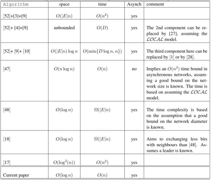
first several entrees show the results of using (to generate an MST algorithm automatically) the known trans-former of Katz and Perry [52], that extends automatically non self stabilizing algorithms to become self stabiliz-ing. The transformer of Katz and Perry [52] assumes a leader whose memory must hold a snapshot of the whole network. The time of the resulting self-stabilizing MST algorithm is O(n) and the memory size is O(|E|n). We have attributed a higher time to [52] in the table, since we wanted to remove its assumption of a known leader, to make a fair comparison to the later papers who do not rely on this assumption.
To remove the assumption, in the first entry we assumed the usage of the only leader election known at the time of [52]. That is, in [3], the first self-stabilizing leader election algorithm was proposed in order to remove the assumptions of [52] that a leader and a spanning tree are given. The combination of [3] and [52] implied a self-stabilizing MST in O(n2) time. (Independently, a leader election algorithm was also presented by [6]; however, we cannot use it here since it needed an extra assumption that a bound on n was known; also, its higher time complexity would have driven the complexity of the transformed MST algorithm higher than the O(n2) stated above.)
Using unbounded space, the time of self-stabilizing leader election was later improved even to O(D) (the actual diameter) [4, 27]. The bounded memory algorithms of [10] or [1, 28], together with [52] and [9], yield a self-stabilizing MST algorithm using O(n|E| log n) bits per node and time O(D log n) or O(n).
Antonoiu and Srimani [5] presented a self stabilizing algorithm whose complexities were not analyzed. As mentioned by [48], the model in that paper can be transformed to the models of the other papers surveyed here, at a high translation costs. Hence, the complexities of the algorithm of [5] may grow even further when stated in these models. Gupta and Srimani [47] presented an O(n log n) bits algorithm. Higham and Liang [48] improved the core memory requirement to O(log n), however, the time complexity went up again to Ω(n|E|). An algorithm with a similar time complexity and a similar memory per node was also presented by Blin, Potop-Butucaru, Rovedakis, and Tixeuil [18]. This latter algorithm exchanges less bits with neighbours than does the algorithm of [48]. The algorithm of [18] addressed also another goal- even during stabilization it is loop free. That is, it also maintains a tree at all times (after reaching an initial tree). This algorithm assumes the existence of a unique leader in the network (while the algorithm in the current paper does not). However, this does not seem to affect the order of magnitude of the time complexity.
Note that the memory size in the last two algorithms above is the same as in the current paper. However, their time complexity is O(|E|n) versus O(n) in the current paper. The time complexity of the algorithm of Blin, Dolev, Potop-Butucaru, and Rovedakis [17] improved the time complexity of [18, 48] to O(n2) but at the cost of growing the memory usage to O(log2n). This may be the first paper using labeling schemes for the design of a self-stabilizing MST protocol, as well as the first paper implementing the algorithm by Gallager, Humblet, and Spira in a self-stabilizing manner without using a general transformer.
Additional studies about MST verification in various models appeared in [26, 30, 31, 53, 54, 55]. In particular, Kor et al. [53] shows that the verification from scratch (without labels) of an MST requires Ω(√n + D) time and Ω(|E|) messages, and that these bounds are tight up to poly-logarithmic factors. We note that the memory complexity was not considered in [53], and indeed the memory used therein is much higher than the one used in the current paper. The time lower bound proof in [53] was later extended in [26] to apply for a variety of verification and computation tasks.
This paper has results concerning distributed verification. Various additional papers dealing with verification have appeared recently, the models of some of them are rather different than the model here. Verification in the LOCAL model (where congestion is abstracted away) was studied in [37] from a computational complexity per-spective. That paper presents various complexity classes, shows separation between them, and provides complete problems for these classes. In particular, the class NLD defined therein exhibits similarities to the notion of proof labeling schemes. Perhaps the main result in [37] is a sharp threshold for the impact of randomization on local
Table 1: Comparing self-stabilizing MST construction algorithms
Algorithm space time Asynch comment
[52]+[3]+[9] O(|E|n) O(n2) yes
[52]+ [4]+[9] unbounded O(D) yes The 2nd component can be
re-placed by [27], assuming the LOCAL model.
[52]+ [9]+ [10] O(|E|n) log n O(min{D log n, n}) yes The third component here can be replaced by [1] or by [28].
[47] O(n log n) O(n) no Implies an O(n2) time bound in
asynchronous networks, assum-ing a good bound on the net-work size is known. The time is based on assuming the LOCAL model.
[48] O(log n) Ω(|E|n) yes The time complexity is based
on the assumption that a good bound on the network diameter is known.
[18] O(log n) Ω(|E|n) yes Aims to exchanging less bits
with neighbours than [48]. As-sumes a leader is known.
[17] O(log2(n)) O(n2) yes
decision of hereditary languages. Following that paper, [38] showed that the threshold in [37] holds also for any non-hereditary language, assuming it is defined on path topologies. In addition, [38] showed further limitations of randomness, by presenting a hierarchy of languages, ranging from deterministic, on the one side of the spec-trum, to almost complete randomness, on the other side. Still, in the LOCAL model, [39] studied the impact of assuming unique identifiers on local decision. We stress that the memory complexity was not considered in neither [37] nor in its follow-up papers [38, 39].
1.3 Our results
This paper contains the following two main results.
(1) Solving an open problem posed by Awerbuch and Varghese [15]: In the context of self-stabilization, an open problem posed in [15] is to find a (synchronous) MST verification algorithm whose time complexity is smaller than the MST computation time, yet with a small memory. Our first main result solves this question positively by constructing a time efficient self-stabilizing verification algorithm for an MST while using optimal memory size, that is O(log n) bits of memory per node. More specifically, the verification scheme takes as input a distributed structure claimed to be an MST. If the distributed structure is indeed an MST, and if a marker algorithm properly marked the nodes to allow the verification, and if no faults occur, then our algorithm outputs accept continuously in every node. However, if faults occur (including the case that the structure is not, in fact, an MST, or that the marker did not perform correctly), then our algorithm outputs reject in at least one node. This reject is outputted in time O(log2n) after the faults cease, in a synchronous network. (Recall, lower bounds which are polynomial in n for MST construction are known even for synchronous networks [58, 62].) In asynchronous networks, the time complexity of our verification scheme grows to O(∆ log3n). We also show that Ω(log n) time is necessary if the memory size is restricted to O(log n), even in synchronous networks. Another property of our verification scheme is that if f faults occurred, then, within the required detection time above, they are detected by some node in the O(f log n) locality of each of the faults. Moreover, we present a distributed implementation of the marker algorithm whose time complexity for assigning the labels is O(n), under the same memory size constraint of O(log n) memory bits per node.
(2) Constructing an asynchronous self-stabilizing MST construction algorithm which uses optimal mem-ory (O(log n) bits) and runs in O(n) time: In our second main result, we show how to enhance a known transformer that makes input/output algorithms self-stabilizing. It now takes as input an efficient construction algorithm and an efficient self-stabilizing proof labeling scheme, and produces an efficient self-stabilizing algo-rithm. When used with our verification scheme, the transformer produces a memory optimal self-stabilizing MST construction algorithm, whose time complexity, namely, O(n), is significantly better even than that of previous algorithms. (Recall, the time complexity of previous MST algorithms that used Ω(log2n) memory bits per node was O(n2), and the time for optimal space algorithms was O(n|E|).) Inherited from our verification scheme, our self-stabilising MST construction algorithm also has the following two properties. First, if faults occur after the construction ended, then they are detected by some nodes within O(log2n) time in synchronous networks, or within O(∆ log3n) time in asynchronous ones, and second, if f faults occurred, then, within the required detection time above, they are detected within the O(f log n) locality of each of the faults. We also show how to improve these two properties, at the expense of some increase in the memory.
1.4 Outline
Preliminaries and some examples of simple, yet useful, proof labeling schemes are given in Section 2. An intuition is given in Section 3. A building block is then given in Section 4. Namely, that section describes a synchronous MST construction algorithm in O(log n) bits memory size and O(n) time. Section 5 describes the construction of parts of the labeling scheme. Those are the parts that use labeling schemes of the kind described in [55]- namely, schemes that can be verified in one time unit. These parts use the MST construction (of Section 4) to assign the labels. Sections 6, 7, and 8 describe the remaining part of the labeling scheme. This part is a labeling scheme by itself, but of a new kind. It saves on memory by distributing information. Specifically, Section 6 describes how the labels should look if they are constructed correctly (and if an MST is indeed represented in the graph). The verifications, in the special case that no further faults occur, is described in Section 7. This module verifies (alas, not in constant time) by moving the distributed information around, for a “distributed viewing”. Because the verification is not done in one time unit, it needs to be made self stabilizing. This is done in Section 8. Section 9 presents a lower bound for the time of a proof labeling scheme for MST that uses only logarithmic memory. (Essentially, the proof behind this lower bound is based on a simple reduction, using the rather complex lower bound given in [54].)
The efficient self-stabilizing MST algorithm is given in Section 10. Using known transformers, we combine efficient MST verification schemes and (non-stabilizing) MST construction schemes to yield efficient self-stabilizing schemes. The MST construction algorithm described in Section 4 is a variant of some known time efficient MST construction algorithms. We show there how those can also be made memory efficient (at the time, this complexity measure was not considered), and hence can be used as modules for our optimal memory self-stabilizing MST algorithm.
2
Preliminaries
2.1 Some general definitions
We use rather standard definitions; a reader unfamiliar with these notions may refer to the model descriptions in the rich literature on these subjects. In particular, we use rather standard definitions of self-stabilization (see, e.g. [32]). Note that the assumptions we make below on time and time complexity imply (in self stabilization jargon) a distributed daemon with a very strong fairness. When we speak of asynchronous networks, this implies a rather fine granularity of atomicity. Note that the common self stabilization definitions include the definitions of faults. We also use standard definitions of graph theory (including an edge weighted graph G = (V, E), with weights that are polynomial in n = |V |) to represent a network (see, e.g. [35]). Each node v has a unique identity ID(v) encoded using O(log n) bits. For convenience, we assume that each adjacent edge of each node v has some label that is unique at v (edges at different nodes may have the same labels). This label, called a port-number, is known only to v and is independent of the port-number of the same edge at the other endpoint of the edge. (Clearly, each port-number can be assumed to be encoded using O(log n) bits). Moreover, the network can store an object such as an MST (Minimum Spanning Tree) by having each node store its component of the representation. A component c(v) at a node v includes a collection of pointers (or port-numbers) to neighbours of v, and the collection of the components of all nodes induces a subgraph H(G) (an edge is included in H(G) if and only if at least one of its end-nodes points at the other end-node). In the verification scheme considered in this current paper, H(G) is supposed to be an MST and for simplicity, we assume that the component of each node contains a single pointer (to the parent, if that node is not defined as the root). It is not difficult to extend our verification scheme to hold also for the case where each component can contain several pointers. Note that the definitions in this paragraph imply a lower bound of Ω(log n) bits on the memory required at each node to
even represent an MST (in graphs with nodes of high degree).
Some additional standard ([40]) parts of the model include the assumption that the edge weights are distinct. As noted often, having distinct edge weights simplifies our arguments since it guarantees the uniqueness of the MST. Yet, this assumption is not essential. Alternatively, in case the graph is not guaranteed to have distinct edge weights, we may modify the weights locally as was done in [53]. The resulted modified weight function ω0(e) not only assigns distinct edge weights, but also satisfies the property that the given subgraph H(G) is an MST of G under ω(·) if and only if H(G) is an MST of G under ω0(·).1
We use the (rather common) ideal time complexity which assumes that a node reads all of its neighbours in at most one time unit, see e.g. [18, 17]. Our results translate easily to an alternative, stricter, contention time complexity, where a node can access only one neighbour in one time unit. The time cost of such a translation is at most a multiplicative factor of ∆, the maximum degree of a node (it is not assumed that ∆ is known to nodes). As is commonly assumed in the case of self-stabilization, each node has only some bounded number of memory bits available to be used. Here, this amount of memory is O(log n).
2.2 Using protocols designed for message passing
We use a self stabilizing transformer of Awerbuch and Varghese as a building block [15]. That protocol was designed for the message passing model. Rather than modifying that transformer to work on the model used here (which would be very easy, but would take space), we use emulation. That is, we claim that any self stabilizing protocol designed for the model of [15] (including the above transformer) can be performed in the model used here, adapted from [18, 17]. This is easy to show: simply use the current model to implement the links of the model of [15]. To send a message from node v to its neighbour u, have v write its shared variable that (only v and) u can read. This value can be read by u after one time unit in a synchronous network as required from a message arrival in the model of [15]. Hence, this is enough for synchronous networks.
In an asynchronous network, we need to work harder to simulate the sending and the receiving of a message, but only slightly harder, given known art. Specifically, in an asynchronous network, an event occurs at u when this message arrives. Without some additional precaution on our side, u could have read this value many times (per one writing) resulting in duplications: multiple message “arriving” while we want to emulate just one message. This is solved by a self stabilizing data link protocol, such as the one used by [3], since this is also the case in a data link protocol in message passing systems where a link may loose a package. There, a message is sent repeatedly, possibly many times, until an acknowledgement from the receiver tells the sender that the message
1
We note, the standard technique (e.g., [40]) for obtaining unique weights is not sufficient for our purposes. Indeed, that technique orders edge weights lexicographically: first, by their original weight ω(e), and then, by the identifiers of the edge endpoints. This yields a modified graph with unique edge weights, and an MST of the modified graph is necessarily an MST of the original graph. For construction purposes it is therefore sufficient to consider only the modified graph. Yet, this is not the case for verification purposes, as the given subgraph can be an MST of the original graph but not necessarily an MST of the modified graph. While the authors in [53] could not guarantee that any MST of the original graph is an MST of the modified graph (having unique edge weights), they instead make sure that the particular given subgraph T is an MST of the original graph if and only if it is an MST of modified one. This condition is sufficient for verification purposes, and allows one to consider only the modified graph. For completeness, we describe the weight-modification in [53]. To obtain the modified graph, the authors in [53] employ the technique, where edge weights are lexicographically ordered as follows. For an edge e = (v, u) connecting v to its neighbour u, consider first its original weight ω(e), next, the value 1 − Yuvwhere Yuvis the
indicator variable of the edge e (indicating whether e belongs to the candidate MST to be verified), and finally, the identifiers of the edge endpoints, ID(v) and ID(u) (say, first comparing the smaller of the two identifiers of the endpoints, and then the larger one). Formally, let ω0(e) = hω(e), 1 − Yv
u, IDmin(e), IDmax(e)i , where IDmin(e) = min{ID(v), ID(u)} and IDmax(e) = max{ID(v), ID(u)}.
Under this weight function ω0(e), edges with indicator variable set to 1 will have lighter weight than edges with the same weight under ω(e) but with indicator variable set to 0 (i.e., for edges e1 ∈ T and e2 ∈ T such that ω(e/ 1) = ω(e2), we have ω0(e1) < ω0(e2)). It
follows that the given subgraph T is an MST of G under ω(·) if and only if T is an MST of G under ω0(·). Moreover, since ω0(·) takes into account the unique vertex identifiers, it assigns distinct edge weights.
arrived. The data link protocol overcomes the danger of duplications by simply numbering the messages modulo some small number. That is, the first message is sent repeatedly with an attached “sequence number” zero, until the first acknowledgement arrives. All the repetitions of the second message have as attachments the sequence number 1, etc. The receiver then takes just one of the copies of the first message, one of the copies of the second, etc. A self stabilized implementation of this idea in a shared memory model appears in [3] using (basically, to play the role of the sequence number) an additional shared variable called the “toggle”, which can take one of three values.2 When u reads that the toggle of v changes, u can emulate the arrival of a message. In terms of time complexity, this protocol takes a constant time, and hence sending (an emulated) message still takes a constant time (in terms of complexity only) as required to emulate the notion of ideal time complexity of [18, 17]. Note that the memory is not increased.
2.3 Wave&Echo
We use the well known Wave&Echo (PIF) tool. For details, the readers are referred to [21, 63]. For completeness, we remind the reader of the overview of Wave&Echo when performed over a rooted tree. It is started by the tree root, and every node who receives the wave message forwards it to its children. The wave can carry a command for the nodes. A leaf receiving the wave, computes the command, and sends the output to its parent. This is called an echo. A parent, all of whose children echoed, computes the command itself (possibly using the outputs sent by the children) and then sends the echo (with its own output) to its parent. The Wave&Echo terminates at the root when all the children of the root echoed, and when the root executed the command too.
In this paper, the Wave&Echo activations carry various commands. Let us describe first two of these com-mands, so that they will also help clarify the notion of Wave&Echo and its application. The first example is the command to sum up values residing at the nodes. The echo of a leaf includes its value. The echo of a parent includes the sum of its own value and the sums sent by its children. Another example is the counting of the nodes. This is the same as the sum operation above, except that the initial value at a node is 1. Similarly to summing up, the operation performed by the wave can also be a logical OR.
2.4 Proof labeling schemes
In [54, 55, 46], the authors consider a framework for maintaining a distributed proof that the network satisfies some given predicate Ψ, e.g., that H(G) is an MST. We are given a predicate Ψ and a graph family F (in this paper, if Ψ and F are omitted, then Ψ is MST and F (or F (n)) is all connected undirected weighted graphs with n nodes). A proof labeling scheme (also referred to as a verification algorithm) includes the following two components.
• A marker algorithm M that generates a label M(v) for every node v in every graph G ∈ F .
• A verifier, that is a distributed algorithm V, initiated at each node of a labeled graph G ∈ F , i.e., a graph whose nodes v have labels L(v) (not necessarily correct labels assigned by a marker). The verifier at each node is initiated separately, and at an arbitrary time, and runs forever. The verifier may raise an alarm at some node v by outputting “no” at v.
Intuitively, if the verifier at v raises an alarm, then it detected a fault. That is, for any graph G ∈ F ,
2
That protocol, called “the strict discipline” in [3], actually provides a stronger property (emulating a coarser grained atomicity), not used here.
• If G satisfies the predicate Ψ and if the label at each node v is M(v) (i.e., the label assigned to v by the marker algorithm M) then no node raises an alarm. In this case, we say that the verifier accepts the labels. • If G does not satisfy the predicate Ψ, then for any assignment of labels to the nodes of G, after some finite
time t, there exists a node v that raises an alarm. In this case, we say that the verifier rejects the labels. Note that the first property above concerns only the labels produced by the marker algorithm M, while the second must hold even if the labels are assigned by some adversary. We evaluate a proof labeling scheme (M, V) by the following complexity measures.
• The memory size: the maximum number of bits stored in the memory of a single node v, taken over all the nodes v in all graphs G ∈ F (n) that satisfy the predicate Ψ (and over all the executions); this includes: (1) the bits used for encoding the identity ID(v), (2) the marker memory: number of bits used for constructing and encoding the labels, and (3) the verifier memory: the number of bits used during the operation of the verifier3.
• The (ideal) detection time: the maximum, taken over all the graphs G ∈ F (n) that do not satisfy the predicate Ψ and over all the labels given to nodes of G by adversaries (and over all the executions), of the time t required for some node to raise an alarm. (The time is counted from the starting time, when the verifier has been initiated at all the nodes.)
• The detection distance: for a faulty node v, this is the (hop) distance to the closest node u raising an alarm within the detection time after the fault occurs. The detection distance of the scheme is the maximum, taken over all the graphs having at most f faults, and over all the faulty nodes v (and over all the executions), of the detection distance of v.
• The (ideal) construction-time: the maximum, taken over all the graphs G ∈ F (n) that satisfy the predicate Ψ (and over all the executions), of the time required for the marker M to assign labels to all nodes of G. Unless mentioned otherwise, we measure construction-time in synchronous networks only.
In our terms, the definitions of [54, 55] allowed only detection time complexity 1. Because of that, the verifier of [54, 55] at a node v, could only consult the neighbours of v. Whenever we use such a scheme, we refer to it as a 1-proof labeling scheme, to emphasis its running time. Note that a 1-proof labelling scheme is trivially self-stabilzying. (In some sense, this is because they “silently stabilize” [33], and “snap stabilize” [20].) Also, in [54, 55], if f faults occurred, then the detection distance was f .
2.5 Generalizing the complexities to a computation
In Section 2.4, we defined the memory size, detection time and the detection distance complexities of a veri-fication algorithm. When considering a (self-stabilizing) computation algorithm, we extend the notion of the memory size to include also the bits needed for encoding the component c(v) at each node. Recall, the definition of a component c(v) in general, and the special case of c(v) for MST, are given in Section 2. (Recall, from Sec-tion 2.4, that the size of the component was excluded from the definiSec-tion of memory size for verificaSec-tion because, there, the designer of the verification scheme has no control over the nodes’ components.)
3
Note that we do not include the number of bits needed for storing the component c(v) at each node v. Recall that for simplicity, we assume here that each component contains a single pointer, and therefore, the size of each component is O(log n) bits. Hence, for our purposes, including the size of a component in the memory complexity would not increase the asymptotical size of the memory, anyways. However, in the general case, if multiple pointers can be included in a component, then the number of bits needed for encoding a component would potentially be as large as O(∆ log n). Since, in this case, the verification scheme has no control over the size of the component, we decided to exclude this part from the definition of the memory complexity.
The notions of detection time and the detection distance can be carried to the very common class of self-stabilizing computation algorithms that use fault detection. (Examples for such algorithms are algorithms that have silent stabilization [33].) Informally, algorithms in this class first compute an output. After that, all the nodes are required to stay in some output state where they (1) output the computation result forever (unless a fault occurs); and (2) check repeatedly until they discover a fault. In such a case, they recompute and enter an output state again. Let us term such algorithms detection based self-stabilizing algorithms. We define the detection time for such algorithms to be the time from a fault until the detection. However, we only define the detection time (and the detection distance) for faults that occur after all the nodes are in their output states. (Intuitively, in the other cases, stabilization has not been reached yet anyhow.) The detection distance is the distance from a node where a fault occurred to the closest node that detected a fault.
2.6 Some examples of 1-proof labeling schemes
As a warm-up exercise, let us begin by describing several simple 1-proof labeling schemes, which will be useful later in this paper. The first two examples are taken from [55] and are explained there in more details. The reader familiar with proof labeling schemes may skip this subsection.
◦ Example 1: A spanning tree. (Example SP) Let fspan denote the predicate such that for any input graph G satisfies, fspan(G) = 1 if H(G) is a spanning tree of G, and fspan(G) = 0 otherwise. We now describe an efficient 1-proof labeling scheme (M, V) for the predicate fspanand the family of all graphs. Let us first describe the marker M operating on a “correct instance”, i.e., a graph G where T = H(G) is indeed a spanning tree of G. If there exists a node u whose component does not encode a pointer to any of its adjacent edges (observe that there can be at most one such node), we root T at u. Otherwise, there must be two nodes v and w whose components point at each other. In this case, we root T arbitrarily at either v or w. Note that after rooting T , the component at each non-root node v points at v’s parent. The label given by M to a node v is composed of two parts. The first part encodes the identity ID(r) of the root r of T , and the second part of the label of v encodes the distance (assuming all weights of edges are 1) between v and r in T .
Given a labeled graph, the verifier V operates at a node v as follows: first, it checks that the first part of the label of v agrees with the first part of the labels of v’s neighbours, i.e., that v agrees with its neighbours on the identity of the root. Second, let d(v) denote the number encoded in the second part of v’s label. If d(v) = 0 then V verifies that ID(v) = ID(r) (recall that ID(r) is encoded in the first part of v’s label). Otherwise, if d(v) 6= 0 then the verifier checks that d(v) = d(u) + 1, where u is the node pointed at by the component at v. If at least one of these conditions fails, the verifier V raises an alarm at v. It is easy to get convinced that (M, V) is indeed a 1-proof labeling scheme for the predicate fspanwith memory size O(log n) and construction time O(n).
Remark. Observe that in case T = H(G) is indeed a (rooted) spanning tree of G, we can easily let each node v know which of its neighbours in G are its children in T and which is its parent. Moreover, this can be done using one unit of time and label size O(log n) bits. To see this, for each node v, we simply add to its label its identity ID(v) and the identity ID(u) of its parent u. The verifier at v first verifies that ID(v) is indeed encoded in the right place of its label. It then looks at the label of its parent u, and checks that v’s candidate for being the identity of u is indeed ID(u). Assume now that these two conditions are satisfied at each node. Then, to identify a child w in T , node v should only look at the labels of its neighbours in G and see which of them encoded ID(v) in the designated place of its label.
◦ Example 2: Knowing the number of nodes (Example NumK) Denote by fsizethe boolean predicate such that fsize(G) = 1 if and only if one designated part of the label L(v) at each node v encodes the number of nodes in
G (informally, when fsizeis satisfied, we say that each node ‘knows’ the number of nodes in G). Let us denote the part of the label of v that is supposed to hold this number by L0(v).
In [55], the authors give a 1-proof labeling scheme (M, V) for fsizewith memory size O(log n). The idea behind their scheme is simple. First, the verifier checks that L0(u) = L0(v) for every two adjacent nodes u and v (if this holds at each node then all nodes must hold the same candidate for being the number of nodes). Second, the marker constructs a spanning tree T rooted at some node r (and verifies that this is indeed a spanning tree using the Example SP above). Third, the number of nodes in T is aggregated upwards along T towards its root r, by keeping at the label M(v) of each node v, the number of nodes n(v) in the subtree of T hanging down from v. This again is easily verified by checking at each node v that n(v) = 1 +P
u∈Child(v)n(u), where Child(v) is the set of children of v. Finally, the root verifies that n(r) = L0(r). It is straightforward that (M, V) is indeed a 1-proof labeling scheme for the predicate fsizewith memory size O(log n) and construction time O(n).
◦ Example 3: An upper bound on the diameter of a tree (Example EDIAM) Consider a tree T rooted at r, and let h denote the height of T . Denote by fheightthe boolean predicate such that fheight(T ) = 1 if and only if one designated part of the label L(v) at each node encodes the same value x, where h ≤ x (informally, when fheight is satisfied, we say that each node ‘knows’ an upper bound of 2x on the diameter D of T ). Let us denote the part of the label of v that is supposed to hold this number by L0(v). We sketch a simple 1-proof labeling scheme (M, V) for fheight. First, the verifier checks that L0(u) = L0(v) for every two adjacent nodes u and v (if this holds at each node then all nodes must hold the same value x). Second, similarly to the proof labeling scheme for fspan given in Example SP above, the label in each node v contains the distance d(v) in the tree from v to the root. Each non-root node verifies that the distance written at its parent is one less than the distance written at itself, and the root verifies that the distance written at itself is 0. Finally, each node v verifies also that x ≥ d(v). If no node raises an alarm then x is an upper bound on the height. On the other hand, if the value x is the same at all nodes and x is an upper bound on the height then no node raises an alarm. Hence the scheme is a 1-proof labeling scheme for the predicate fheightwith memory size O(log n) and construction time O(n).
3
Overview of the MST verification scheme and the intuition behind it
The final MST construction algorithm makes use of several modules. The main technical contribution of this paper is the module that verifies that the collection of nodes’ components is indeed an MST. This module in itself is composed of multiple modules. Some of those, we think may be useful by themselves. To help the reader avoid getting lost in the descriptions of all the various modules, we present, in this section, an overview of the MST verification part.
Given a graph G and a subgraph that is represented distributively at the nodes of G, we wish to produce a self-stabilizing proof labeling scheme that verifies whether the subgraph is an MST of G. By first employing the (self-stabilizing) 1-proof labeling scheme mentioned in Example SP, we may assume that the subgraph is a rooted spanning tree of G (otherwise, at least one node would raise an alarm). Hence, from now on, we focus on a spanning tree T = (V (G), E(T )) of a weighted graph G = (V (G), E(G)), rooted at some node r(T ), and aim at verifying the minimality of T .
3.1 Background and difficulties
From a high-level perspective, the proof labeling scheme proves that T could have been computed by an algorithm that is similar to that of GHS, the algorithm of Gallager, Humblet, and Spira’s described in [40]. This leads to a simple idea: when T is a tree computed by such an algorithm, T is an MST. Let us first recall a few terms from
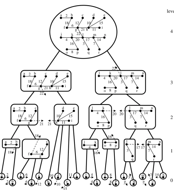
[40]. A fragment F denotes a connected subgraph of T (we simply refer it to a subtree). Given a fragment F , an edge (v, u) ∈ E(G) whose one endpoint v is in F , while the other endpoint u is not, is called outgoing from F . Such an edge of minimum weight is called a minimum outgoing edge from F . A fragment containing a single node is called a singleton. Recall that GHS starts when each node is a fragment by itself. Essentially, fragments merge over their minimum outgoing edges to form larger fragments. That is, each node belongs to one fragment F1, then to a larger fragment F2 that contains F1, etc. This is repeated until one fragment spans the network. A tree constructed in that way is an MST. Note that in GHS, the collection of fragments is a laminar family, that is, for any two fragments F and F0in the collection, if F ∩ F0 6= ∅ then either F ⊆ F0or F0 ⊆ F (see, e.g. [44]). Moreover, each fragment has a level; in the case of v above, F2’s level is higher than that of F1. This organizes the fragments in a hierarchy H, which is a tree whose nodes are fragments, where fragment F1is a descendant in H of F2if F2contains F1. GHS manages to ensure that each node belongs to at most one fragment at each level, and that the total number of levels is O(log n). Hence, the hierarchy H has O(log n) height.
The marker algorithm in our proof labeling scheme performs, in some sense, a reverse operation. If T is an MST, the marker “slices” it back into fragments. Then, the proof labeling scheme computes for each node v:
• The (unique) name of each of the fragments Fjthat v belongs to, • the level of Fj, and
• the weight of Fj’s minimum outgoing edge.
Note that each node participates in O(log n) fragments, and the above “piece of information” per fragment requires O(log n) bits. Hence, this is really too much information to store in one node. As we shall see later, the verification scheme distributes this information and then brings it to the node without violating the memory size bound O(log n). For now, it suffices to know that given these pieces of information and the corresponding pieces of information of their neighbours, the nodes can verify that T could have been constructed by an algorithm similar to GHS. That way, they verify that T is an MST. Indeed, the 1-proof labeling schemes for MST verification given in [54, 55] follow this idea employing memory size of O(log2n) bits. (There, each node keeps O(log n) pieces, each of O(log n) bits.)
The current paper allows each node to hold only O(log n) memory bits. Hence, a node has room for only a constant number of such pieces of information at a time. One immediate idea is to store some of v’s pieces in some other nodes. Whenever v needs a piece, some algorithm should move it towards v. Moving pieces would cost time, hence, realizing some time versus memory size trade-off.
Unfortunately, the total (over all the nodes) number of pieces in the schemes of [54, 55] is Ω(n log n). Any way one would assign these pieces to nodes would result in the memory of some single node needing to store Ω(log n) pieces, and hence, Ω(log2n) bits. Thus, one technical step we used here is to reduce the total number of pieces to O(n), so that we could store at each node just a constant number of such pieces. However, each node still needs to use Ω(log n) pieces. That is, some pieces may be required by many nodes. Thus, we needed to solve also a combinatorial problem: locate each piece “close” to each of the nodes needing it, while storing only a constant number of pieces per node.
The solution of this combinatorial problem would have sufficed to construct the desired scheme in the LOCAL model [61]. There, node v can “see” the storage of nearby nodes. However, in the congestion aware model, one actually needs to move pieces from node to node, while not violating the O(log n) memory per node constraint. This is difficult, since, at the same time v needs to see its own pieces, other nodes need to see their own ones.
3.2 A very high level overview
Going back to GHS, one may notice that its correctness follows from the combination of two properties:
• P1. (Well-Forming) The existence of a hierarchy tree H of fragments, satisfying the following: • Each fragment F ∈ H has a unique selected outgoing edge (except when F is the whole tree T ). • A (non-singleton) fragment is obtained by merging its children fragments in H through their selected
outgoing edges.
• P2. (Minimality) The selected outgoing edge of each fragment is its minimal outgoing edge.
In our proof labeling scheme, we verify the aforementioned two properties separately. In Section 5, we show how to verify the first property, namely, property Well-Forming. This turns out to be a much easier task than verifying the second property. Indeed, the Well-Forming property can be verified using a 1-proof labeling scheme, while still obeying the O(log n) bits per node memory constraint. Moreover, the techniques we use for verifying the Well-Forming are rather similar to the ones described in [55]. The more difficult verification task, namely, verifying the Minimality property P2, is described in Section 6. This verification scheme requires us to come up with several new techniques which may be considered as contributions by themselves. We now describe the intuition behind these verifications.
3.3 Verifying the Well-Forming property (described in detail in Sections 4 and 5)
We want to show that T could have been produced by an algorithm similar to GHS. Crucially, since we care about the memory size, we had to come up with a new MST construction algorithm that is similar to GHS but uses only O(log n) memory bits per node and runs in time O(n). This MST construction algorithm, called SYNC MST, can be considered as a synchronous variant of GHS and is described in Section 4.
Intuitively, for a correct instance (the case T is an MST), the marker algorithm M produces a hierarchy of fragments H by following the new MST construction algorithm described in Section 4. Let ` = O(log n) be the height of H. For a fixed level j ∈ [0, `], it is easy to represent the partition of the tree into fragments of level j using just one bit per node. That is, the root r0 of each fragment F0 of level j has 1 in this bit, while the nodes in F0\ {r0} have 0 in this bit. Note, these nodes in F0\ {r0} are the nodes below r0 (further away from the root of T ), until (and not including) reaching additional nodes whose corresponding bit is 1. Hence, to represent the whole hierarchy, it is enough to attach a string of length ` + 1-bits at each node v. The string at a node v indicates, for each level j ∈ [0, `], whether v is the root of the fragment of level j containing v (if one exists).
Next, still for correct instances, we would like to represent the selected outgoing edges distributively. That is, each node v should be able to detect, for each fragment F containing v, whether v is an endpoint of the selected edge of F . If v is, it should also know which of v’s edges is the selected edge. This representation is used later for verifying the two items of the Well-Forming property specified above. For this purpose, first, we add another string of ` + 1 entries at each node v, one entry per level j. This entry specifies, first, whether there exists a level j fragment Fj(v) containing v. If Fj(v) does exist, the entry specifies whether v is incident to the corresponding selected edge. Note, storing the information at v specifying the pointers to all the selected edges of the fragments containing it, may require O(log2n) bits of memory at v. This is because there may be O(log n) fragments containing v; each of those may select an edge at v leading to an arbitrary neighbour of v in the tree T ; if v has many neighbours, each edge may cost O(log n) bits to encode. The trick is to distribute the information regarding v’s selected edges among v’s children in T . (Recall that v can look at the data structures of v’s children.)
The strings mentioned in the previous paragraphs are supposed to define a hierarchy and selected outgoing edges from the fragments of the hierarchy. However, on incorrect instances, if corrupted, the strings may not
represent the required. For example, the strings may represent more than one selected edge for some fragment. Hence, we need also to attach proof labels for verifying the hierarchy and the corresponding selected edges represented by those strings. Fortunately, for proving the Well-Forming property only, it is not required to verify that the represented hierarchy (and the corresponding selected edges) actually follow the MST construction algorithm (which is the case for correct instances). In Section 5, we present 1-proof labeling schemes to show that the above strings represent some hierarchy with corresponding selected edges, and that the Well-Forming property does hold for that hierarchy.
3.4 Verifying The Minimality property (described in detail in Sections 6, 7 and 8)
A crucial point in the scheme is letting each node v know, for each of its incident edges (v, u) ∈ E and for each level j, whether u and v share the same level j fragment. Intuitively, this is needed in order to identify outgoing edges. For that purpose, we assign each fragment a unique identifier, and v compares the identifier of its own level j fragment to the identifier of u’s level j fragment.
Consider the number of bits required to represent the identifiers of all the fragments that a node v participates in. There exists a method to assign unique identifiers such that this total number is only O(log n) [56, 36]. Unfortunately, we did not manage to use that method here. Indeed, there exists a marker algorithm that assigns identifiers according to that method. However, we could not find a low space and short time method for the verifier to verify that the given identifiers of the fragments were indeed assigned in that way. (In particular, we could not verify efficiently that the given identifiers are indeed unique).
Hence, we assign identifiers according to another method that appears more memory wasteful, where the identity ID(F ) of a fragment F is composed of the (unique) identity of its root together with its level. We also need each node v to know the weight ω(F ) of the minimum outgoing edge of each fragment F containing v. To summarize, the piece of information I(F ) required in each node v per fragment F containing v is ID(F ) ◦ ω(F ). Thus, I(F ) can be encoded using O(log n) bits. Again, note that since a node may participate in ` = Θ(log n) fragments, the total number of bits used for storing all the I(F ) for all fragments F containing v would thus be Θ(log2n). Had no additional steps been taken, this would have violated the O(log n) memory constraint.
Luckily, the total number of bits needed globally for representing the pieces I(F ) of all the fragments F is only O(n log n), since there are at most 2n fragments, and I(F ) of a fragment F is of size O(log n) bits. The difficulty results from the fact that multiple nodes need replicas of the same information. (E.g., all the nodes in a fragment need the ID of the fragment.) If a node does not store this information itself, it is not clear how to bring all the many pieces of information to each node who needs them, in a short time (in spite of congestion) and while having only a constant number of such pieces at a node at each given point in time.
To allow some node v to check whether its neighbour u belongs to v’s level j fragment Fj(v) for some level j, the verifier at v needs first to reconstruct the piece of information I(Fj(v)). Intuitively, we had to distribute the information, so that I(F ) is placed “not too far” from every node in F . To compare I(Fj(v)) with a neighbour u, node v must also obtain I(Fj(u)) from u. This requires some mechanism to synchronize the reconstructions in neighbouring nodes. Furthermore, the verifier must be able to overcome difficulties resulting from faults, which can corrupt the information stored, as well as the reconstruction and the synchronization mechanisms.
The above distribution of the I’s is described in Section 6. The distributed algorithm for the “fragment by fragment” reconstruction (and synchronization) is described in Section 7. The required verifications for validating the I’s and comparing the information of neighbouring nodes are described in Section 8.
3.4.1 Distribution of the pieces of information (described in detail in Section 6)
At a very high level description, each node v stores permanently I(F ) for a constant number of fragments F . Using that, I(F ) is “rotated” so that each node in F “sees” I(F ) in O(log n) time. We term the mechanism that performs this rotation a train. A first idea would have been to have a separate train for each fragment F that would “carry” the piece I(F ) and would allow all nodes in F to see it. However, we did not manage to do that efficiently in terms of time and of space. That is, one train passing a node could delay the other trains that “wish” to pass it. Since neighbouring nodes may share only a subset of their fragments, it is not clear how to pipeline the trains. Hence, those delays could accumulate. Moreover, as detailed later, each train utilizes some (often more than constant) memory per node. Hence, a train per fragment would have prevented us from obtaining an O(log n) memory solution.
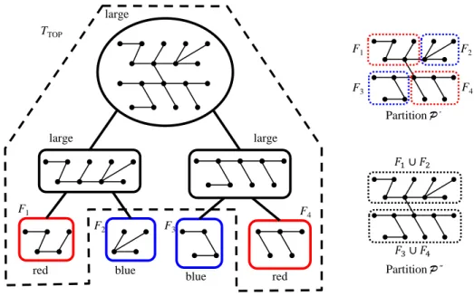
A more refined idea would have been to partition the tree into connected parts, such that each part P intersects O(|P |) fragments. Using such a partition, we could have allocated the O(|P |) pieces (of these O(|P |) fragments), so that each node of P would have been assigned only a constant number of such pieces, costing O(log n) bits per node. Moreover, just one train per part P could have sufficed to rotate those pieces among the nodes of P . Each node in P would have seen all the pieces I(F ) for fragments F containing it in O(|P |) time. Hence, this would have been time efficient too, had P been small.
Unfortunately, we did not manage to construct the above partition. However, we managed to obtain a similar construction: we construct two partitions of T , called Top and Bottom. We also partitioned the fragments into two kinds: top and bottom fragments. Now, each part P of partition Top intersects with O(|P |) top fragments (plus any number of bottom fragments). Each part P of partition Bottom intersects with O(|P |) bottom frag-ments (plus top fragfrag-ments that we do not count here). For each part in Top (respectively Bottom), we shall distribute the information regarding the O(|P |) top (respectively, bottom) fragments it intersects with, so that each node would hold at most a constant number of such pieces of information. Essentially, the pieces of in-formation regarding the corresponding fragments are put in the nodes of the part (permanently) according to a DFS (Depth First Search) order starting at the root of the part. For any node v, the two parts containing it encode together the information regarding all fragments containing v. Thus, to deliver all relevant information, it suffices to utilize one train per part (and hence, each node participates in two trains only). Furthermore, the partitions are made so that the diameter of each part is O(log n), which allows each train to quickly pass in all nodes, and hence to deliver the relevant information in short time.
The distributed implementation of this distribution of pieces of information, and, in particular, the distributed construction of the two partitions, required us to come up with a new multi-wave primitive, enabling an efficient (in O(n)) time) parallel (i.e., pipelined) executions of Wave&Echo operations on all fragments of Hierarchy HM.
3.4.2 Viewing the pieces of information (described in detail in Section 7)
Consider a node v and a fragment Fj(v) of level j containing it. Recall that the information I(Fj(v)) should reside in some node of a part P to which v belongs. To allow v to compare I(Fj(v)) to I(Fj(u)) for a neighbour u, both these pieces must somehow be “brought” to v. The process handling this task contains several compo-nents. The first component is called the train which is responsible for moving the pieces of information through P ’s nodes, such that each node does not hold more than O(log n) bits at a time, and such that in short time, each node in P “sees” all pieces, and in some prescribed order. Essentially, a train is composed of two ingredients. The first ingredient called convergecast pipelines the pieces of information in a DFS order towards the root of the part (recall, the pieces of information of the corresponding fragments are initially located according to a DFS order). The second ingredient broadcasts the pieces from the root of the part to all nodes in the part. Since the number of pieces is O(log n) and the diameter of the part is O(log n), the synchronous environment guarantees
that each piece of information is delivered to all nodes of a part in O(log n) time. On the other hand, in the asyn-chronous environment some delays may occur, and the delivery time becomes O(log2n). These time bounds are also required to self-stabilize the trains, by known art, see, e.g. [23, 20].
Unfortunately, delivering the necessary pieces of information at each node is not enough, since I(Fj(v)) may arrive at v at a different time than I(Fj(u)) arrives at u. Recall that u and its neighbour v need to have these pieces simultaneously in order to compare them (to know whether the edge e = (u, v) is outgoing from Fj(v)).
Further complications arise from the fact that the neighbours of a node v may belong to different parts, so different trains pass there. Note that v may have many neighbours, and we would not want to synchronize so many trains. Moreover, had we delayed the train at v for synchronization, the delays would have accumulated, or even would have caused deadlocks. Hence, we do not delay these trains. Instead, v repeatedly samples a piece from its train, and synchronizes the comparison of this piece with pieces sampled by its neighbours, while both trains advance without waiting. Perhaps not surprisingly, this synchronization turns out to be easier in synchronous networks, than in asynchronous ones. Our synchronization mechanism guarantees that each node can compare all pieces I(Fj(v)) with I(Fj(u)) for all neighbours u and levels j in a short time. Specifically, O(log2n) time in synchronous environments and O(∆ log3n) time in asynchronous ones.
3.4.3 Local verifications (described in detail in Section 8)
So far, with respect to verifying the Minimality property, we have not discussed issues of faults that may com-plicate the verification. Recall, the verification process must detect if the tree is not an MST. Informally, this must hold despite the fact that the train processes, the partitions, and also, the pieces of information carried by the trains may be corrupted by an adversary. For example, the adversary may change or erase some (or even all) of such pieces corresponding to existing fragments. Moreover, even correct pieces that correspond to existing fragments may not arrive at a node in the case that the adversary corrupted the partitions or the train mechanism. In Section 8, we explain how the verifier does overcome such undesirable phenomena, if they occur. In-tuitively, what is detected is not necessarily the fact that a train is corrupted (for example). Instead, what is detected is the state that some part is incorrect (either the tree is not an MST, or the train is corrupted, or ... etc.). Specifically, we show that if an MST is not represented in the network, this is detected in time O(log2n) for synchronous environments and time O(∆ log3n) for asynchronous ones. Note that for a verifier, the ability to detect while assuming any initial configuration means that the verifier is self-stabilizing, since the sole purpose of the verifier is to detect.
Verifying that some two partitions exist is easy. However, verifying that the given partitions are as described in Section 6.1, rather than being two arbitrary partitions generated by an adversary seems difficult. Fortunately, this verification turns out to be unnecessary.
First, as mentioned, it is a known art to self-stabilize the train process. After trains stabilize, we verify that the set of pieces stored in a part (and delivered by the train) includes all the (possibly corrupted) pieces of the form I(Fj(v)), for every v in the part and for every j such that v belongs to a level j fragment. Essentially, this is done by verifying at the root r(P ) of a part P , that (1) the information regarding fragments arrives at it in a cyclic order (the order in which pieces of information are supposed to be stored in correct instances), (2) the levels of pieces arriving at r(P ) comply with the levels of fragments to which r(P ) belongs to, as indicated by r(P )’s data-structure. Next, we verify that the time in which each node obtains all the pieces it needs is short. This is guaranteed by the correct train operation, as long as the diameter of parts is O(log n), and the number of pieces stored permanently at the nodes of the part is O(log n). Verifying these two properties is accomplished using a 1-proof labelling scheme of size O(log n), similarly to the schemes described in Examples 2 and 3 (SP and EDIAM, mentioned in Section 2.6).
Finally, if up to this point, no node raised an alarm, then for each node v, the (possibly corrupted) pieces of information corresponding to v’s fragments reach v in the prescribed time bounds. Now, by the train synchro-nization process, each node can compare its pieces of information with the ones of its neighbours. Hence, using similar arguments as was used in the O(log2n)-memory bits verification scheme of [55], nodes can now detect the case that either one of the pieces of information is corrupted or that T is not an MST.
4
A synchronous MST construction in O(log n) bits memory size and O(n) time
In this section, we describe an MST construction algorithm, called SYNC MST, that is both linear in its running time and memory optimal, that is, it runs in O(n) time and has O(log n) memory size. We note that this algorithm is not self-stabilizing and its correct operation assumes a synchronous environment. The algorithm will be useful later for two purposes. The first is for distributively assigning the labels of the MST proof labelling scheme, as described in the next section. The second purpose, is to be used as a module in the self-stabilizing MST construction algorithm.
As mentioned, the algorithm of Gallager, Humblet, and Spira (GHS) [40] constructs an MST in O(n log n) time. This has been improved by Awerbuch to linear time, using a somewhat involved algorithm. Both algorithms are also efficient in terms of the number of messages they send. The MST construction algorithm described in this section is, basically, a simplification of the GHS algorithm. There are two reasons for why we can simplify that algorithm, and even get a better time complexity. The first reason is that our algorithm is synchronous, whereas GHS (as well as the algorithm by Awerbuch) is designed for asynchronous environments. Our second aid is the fact that we do not care about saving messages (anyhow, we use a shared memory model), while the above mentioned algorithms strive to have an optimal message complexity. Before describing our MST construction algorithm, we recall the main features of the GHS algorithm.
4.1 Recalling the MST algorithm of Gallager, Humblet, and Spira (GHS)
For full details of GHS, please refer to [40]. GHS uses connected subgraphs of the final MST, called fragments. Each node in a fragment, except for the fragment’s root, has a pointer to its parent in the fragment. When the algorithm starts, every node is the root of the singleton fragment including only itself. Each fragment is associated with its level (zero for a singleton fragment) and the identity of its root (this is a slight difference from the description in [40], where a fragment is said to be rooted at an edge). Each fragment F searches for its minimum outgoing edge emin(F ) = (v, u). Using the selected edges, fragments are merged to produce larger fragments of larger levels. That is, two or more fragments of some level j, possibly together with some fragments of levels lower than j, are merged to create a fragment of level j + 1. Eventually, there remains only one fragment spanning the graph which is an MST.
In more details, each fragment sends an offer (over emin(F )) to merge with the other fragment F0, to which the other endpoint u belongs. If F0 is of a higher level, then F is connected to F0. That is, the edges in F are reoriented so that F is now rooted in the endpoint v of emin(F ), which becomes a child of the other endpoint u.
If the level of F0 is lower, then F waits until the level of F0 grows (see below, the description of “test” messages). The interesting case is when F and F0 are of the same level j. If emin(F ) = emin(F0), then F and F0merge to become one fragment, rooted at, say, the highest ID node between u and v. The level of the merged fragment is set to j + 1.
The remaining case, that (w.l.o.g.) w(emin(F )) > w(emin(F0)) does not need a special treatment. When F sends F0 an offer to merge, F0 may have sent such an offer to some F00 over w(emin(F0)). Similarly, F00 may have sent an offer to some F000(over w(emin(F00))), etc. No cycle can be created in this chain of offers (because