Glossy Probe Reprojection for Interactive Global Illumination
Texte intégral
Figure

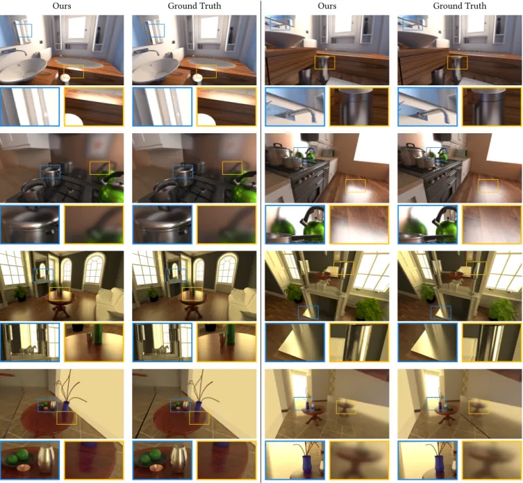
![Fig. 17. Comparisons with same frame rate for each method. Previous methods: [Robison and Shirley 2009], [McGuire et al](https://thumb-eu.123doks.com/thumbv2/123doknet/13553381.419642/14.918.83.846.117.408/comparisons-frame-method-previous-methods-robison-shirley-mcguire.webp)
Documents relatifs
To achieve fast or even interactive updates, we first use the line-space hier- archy for incremental updates of the diffuse transport, and then restrict the number of particles
Point based rendering methods represent the scene’s geometry as a set of point samples, that is object space position, surface normal and material data.. Usually, the point samples
The energy corresponding to each photon im- pact is associated to regions of space, defined by points and used during the rendering phase as virtual surface element light
L’archive ouverte pluridisciplinaire HAL, est destinée au dépôt et à la diffusion de documents scientifiques de niveau recherche, publiés ou non, émanant des
`a notre probl´ematique au paragraphe A.3.2. Puis, nous pr´esentons une nouvelle m´ethode pour le rendu sur GPU des reflets sp´eculaires `a l’aide d’une hi´erarchie de rayons
In particular we list the different scenes with the ε ac- curacy threshold (see Section 4.2), and the corresponding number of directional distribution basis functions used for
The rendering equation [28] is a simple formulation of the global illumination problem as an integral equation. It describes the equilibrium of light exchange in a scene,
est également possible de se baser sur des périodes libres observées pour estimer le nombre de n÷uds actifs dans un réseau sans l où tous les n÷uds sont dans la même zone
