HAL Id: hal-01620389
https://hal.inria.fr/hal-01620389
Submitted on 23 Nov 2017
HAL is a multi-disciplinary open access
archive for the deposit and dissemination of
sci-entific research documents, whether they are
pub-lished or not. The documents may come from
L’archive ouverte pluridisciplinaire HAL, est
destinée au dépôt et à la diffusion de documents
scientifiques de niveau recherche, publiés ou non,
émanant des établissements d’enseignement et de
Minimum Size Tree-Decompositions
Bi Li, Fatima Zahra Moataz, Nicolas Nisse, Karol Suchan
To cite this version:
Bi Li, Fatima Zahra Moataz, Nicolas Nisse, Karol Suchan. Minimum Size Tree-Decompositions.
Discrete Applied Mathematics, Elsevier, 2017, �10.1016/j.dam.2017.01.030�. �hal-01620389�
Minimum Size Tree-Decompositions
I,IIBi Lic, Fatima Zahra Moatazb,a, Nicolas Nissea,b, Karol Suchand,e
aInria, France
bUniv. Nice Sophia Antipolis, CNRS, I3S, UMR 7271, Sophia Antipolis, France cSchool of Mathematics and statistics, Xidian University, Xi’an, China
dUniversidad Adolfo Ib´a˜nez, Santiago, Chile eAGH University of Science and Technology, Krakow, Poland
Abstract
We study in this paper the problem of computing a tree-decomposition of a graph with width at most k and minimum number of bags. More precisely, we focus on the following problem: given a fixed k ≥ 1, what is the complexity of computing a tree-decomposition of width at most k with minimum number of bags in the class of graphs with treewidth at most k? We prove that the problem is NP-complete for any fixed k ≥ 4 and polynomial for k ≤ 2; for k = 3, we show that it is polynomial in the class of trees and 2-connected outerplanar graphs.
1. Introduction
A tree-decomposition of a graph [15] G is a way to represent G by a family of sub-sets of its vertex-set organized in a tree-like manner and satisfying some connectivity property. The treewidth of G measures the proximity of G to a tree. More formally, a tree-decomposition of G = (V, E) is a pair (T, X ) where X = {Xt|t ∈ V (T )} is a
family of subsets of V , called bags, and T is a tree, such that:
• S
t∈V (T )Xt= V ;
• for any edge uv ∈ E, there is a bag Xt(for some node t ∈ V (T )) containing
both u and v;
• for any vertex v ∈ V , the set {t ∈ V (T )|v ∈ Xt} induces a subtree of T .
The width of a tree-decomposition (T, X ) is maxt∈V (T )|Xt| − 1 and its size is the
order |V (T )| of T . The treewidth of G, denoted by tw(G), is the minimum width over
IThis work has been partially supported by European Project FP7 EULER, ANR project Stint
(ANR-13-BS02-0007), the associated Inria team AlDyNet, the project ECOS-Sud Chile and a grant from the ”Conseil r´egional Provence Alpes-Cˆote d’Azur”.
IIAn extended abstract of this paper has been published in the proceedings of the 8th Latin-American
Algorithms, Graphs and Optimization Symposium (LAGOS 2015)[13]
∗Please address correspondence to Nicolas Nisse
all possible tree-decompositions of G. If T is constrained to be a path, (T, X ) is called a path-decomposition of G. The pathwidth of G, denoted by pw(G), is the minimum width over all possible path-decompositions of G.
Tree-decompositions are the corner-stone of many dynamic programming algo-rithms for solving graph problems. For example, the famous Courcelle’s Theorem states that any problem expressible in MSOL can be solved in linear-time in the class of bounded treewidth graphs [7]. Another framework based on graph decompositions is the bi-dimensionality theory that allowed the design of sub-exponential-time algo-rithms for many problems in the class of graphs excluding some fixed graph as a minor (e.g., [8]). Given a tree-decomposition with width w and size n, the time-complexity of most of such dynamic programming algorithms can often be expressed as O(2wn)
or O(2w log wn). These algorithms have mainly theoretical interest because their
time-complexity depends exponentially on the treewidth and, on the other hand, no practical algorithms are known to compute a good tree-decomposition for graphs with treewidth at least 5.
Since the computation of tree-decompositions is a challenging problem, we propose in this article to study it from a new point of view. Namely, we aim at minimizing the number of bags of the tree-decomposition when the width is bounded. This new perspective is interesting on its own and we hope it will allow to gain more insight into the difficulty of designing practical algorithms for computing tree-decompositions.
We consider the problem of computing tree-decompositions with minimum size. If the width is not constrained, then a trivial solution is a tree-decomposition of the graph with one bag (the full vertex-set). Hence, given a graph G and an integer k ≥ tw(G), we consider the problem of minimizing the size of a tree-decomposition of G with width at most k.
Related work. The problem of computing ”good” tree-decompositions has been ex-tensively studied. Computing optimal tree-decomposition - i.e., with width tw(G) - is NP-complete in the class of general graphs G [1]. For any fixed k ≥ 1, Bodlaender designed an algorithm that computes, in time O(kk3n), a tree-decomposition of width k of any n-vertex graph with treewidth at most k [3]. Recently, a single-exponential (in k) algorithm has been proposed that computes a tree-decomposition with width at most 5k in the class of graphs with treewidth at most k [4]. As far as we know, the only practical algorithms for computing optimal tree-decompositions hold for graphs with treewidth at most 1 (trivial since tw(G) = 1 if and only if G is a tree), 2 (graphs excluding K4as a minor) [18], 3 [2, 12, 14] and 4 [16].
In [9], Dereniowski et al. consider the problem of minimum size path-decompositions. Given any positive integer k and any graph G with pathwidth at most k, let lk(G) denote the smallest size (length) of a path-decomposition of G
with width at most k. For any fixed k ≥ 4, computing lkis NP-complete in the class
of general graphs and it is NP-complete, for any fixed k ≥ 5, in the class of con-nected graphs [9]. Moreover, computing lk can be solved in polynomial-time in the
class of graphs with pathwidth at most k for any k ≤ 3. Finally, the ”dual” prob-lem is also hard: for any fixed l ≥ 2, it is NP-complete in general graphs to compute
the minimum width of a path-decomposition with length l [9]1. We have generalized
the problem of minimum size path-decomposition presented in [9], and introduced the problem of minimum size tree-decomposition in a shorter version of this paper [13]. To the best of our knowledge, no other paper has dealt with the computation of tree-decompositions with minimum size before [13]. However, very recently, following the work in [13] and [9], Bodlaender et al. [6] have proposed exact subexponential time algorithms to solve the problems of minimum size tree-decomposition and minimum size path-decomposition for a fixed width k in 2O(n/ log(n)) time and showed that the two problems cannot be solved in 2o(n/ log(n))time, assuming the Exponential Time
Hypothesis.
Contribution. Let k be any positive integer and G be any graph. If tw(G) > k, let us set sk(G) = ∞. Otherwise, let sk(G) denote the minimum size of a
tree-decomposition of G with width at most k. See a simple example in Figure 1. We first prove in Section 2 that, for any (fixed) k ≥ 4, the problem of computing sk is
NP-hard in the class of graphs with treewidth at most k. Moreover, the computation of sk for k ≥ 5 is NP-hard in the class of connected graphs with treewidth at most
k. Furthermore, the computation of s4 is NP-complete in the class of planar graphs
with treewidth 3. In Section 3, we present a general approach for computing sk for
any k ≥ 1. In the rest of the article, we prove that computing s2 can be solved in
polynomial-time, and show that s3can be computed in polynomial-time in the class of
trees and 2-connected outerplanar graphs.
Figure 1: Given a tree G with five vertices, for any k ≥ 1, a minimum size tree-decomposition of width at most k is illustrated: s1(G) = 4, s2(G) = s3(G) = 2, and sk>3(G) = 1.
2. NP-hardness in the class of bounded treewidth graphs
In this section, we prove that:
1This result proved for path-decompositions can be straightforwardly extended to tree-decompositions,
i.e. for any fixed s ≥ 2, it is NP-complete in general graphs to compute the minimum width of a tree-decomposition with size s.
Theorem 1. For any fixed integer k ≥ 4 (resp., k ≥ 5), the problem of computing skis
NP-complete in the class of graphs (resp., of connected graphs) with treewidth at most k.
Note that the corresponding decision problem is clearly in NP. Hence, we only need to prove it is NP-hard.
Our proof mainly follows the one of [9] for minimum size path-decompositions. Hence, we recall here the two steps of the proof in [9]. First, it is proved that, if computing lkis NP-hard for any k ≥ 1 in general graphs, then the computation of lk+1
is NP-hard in the class of connected graphs. Second, it is shown that computing l4is
NP-hard in general graphs with pathwidth 4. In particular, this implies that computing l5 is NP-hard in the class of connected graphs with pathwidth 5. The second step
consists of a reduction from the 3-PARTITION problem [10] to the one of computing l4. Precisely, for any instance I of 3-PARTITION, a graph GIis built such that I is a
YES instance if and only if l4(GI) equals a defined value `I.
Our contribution consists first in showing that the first step of [9] directly extends to the case of tree-decompositions. That is, it directly implies that, if computing skis
NP-hard for some k ≥ 4 in general graphs, then so is the computation of sk+1in the
class of connected graphs. Our main contribution of this section is to show that, for the graphs GIbuilt in the reduction proposed in [9], any tree-decomposition of GI with
width at most 4 and minimum size is a path-decomposition. Hence, in this class of graphs, l4 = s4and, for any instance I of 3-PARTITION, I is a YES instance if and
only if s4(GI) equals a defined value `I. We describe the details in what follows.
Lemma 2. If the problem of computing sk for an integerk ≥ 1 is NP-complete in
general graphs, then the computation ofsk+1is NP-complete in the class of connected
graphs.
Proof. Let G be any graph. We construct an auxiliary connected graph G0from G by adding a vertex a adjacent to all vertices in V (G). Given two integers k, s ≥ 1, in the following, we prove that there is a tree-decomposition of G with width at most k and size at most s if and only if there is a tree-decomposition of G0with width at most k + 1 and size at most s.
First, let us assume that (T, X ) is a tree-decomposition of G with width at most k and size at most s. By adding a in each bag of X , we obtain a tree-decomposition of G0with width at most k + 1 and size at most s.
Now let (T0, X0) be a tree-decomposition of G0with width at most k + 1 and size at
most s. We are going to find a tree-decomposition of G with width at most k and size at most s. Let Xabe the set of all bags in X0containing a. Let Tabe the subtree of T0
induced by the bags in Xa. Every vertex v ∈ V (G) is contained in a bag in Xabecause
va ∈ E(G0). For any edge uv ∈ E(G), there is a bag X ⊇ {a, u, v} in X0 since {a, u, v} induces a clique in G0. This implies that X ∈ X
a. We delete a from each bag
of Xaand denote by X−the obtained set of bags. So (Ta, X−) is a tree-decomposition
of G with width at most k and size at most s.
Before doing the reduction from the 3-PARTITIONproblem to the problem of com-puting s4, let us first recall its definition.
3 i,1 K 3 i,2 K 3 i,3 K 4 i,1 K 4 i,2 K (a) Hi, where wi= 3 5 1 K 5 2 K 5 3 K 4 1 P 4 2 P (b) H2,4
Figure 2: Examples of gadgets in graph G(S, b) [9]
Definition 1. [3-PARTITION]
Instance: A setS of 3m positive integers S = (w1, . . . , w3m) and an integer b.
Question: Is there a partition of the set{1, . . . , 3m} into m sets S1, . . . , Smsuch that
P
i∈Sjwi= b for each j = 1, . . . , m?
This problem is NP-complete even if |Sj| = 3 for all j = 1, . . . , m [10].
Given an instance of 3-PARTITION, in the following, we construct a disconnected graph G(S, b) as in [9]. First, for each i ∈ {1, . . . , 3m}, we construct a connected graph Hias follows. We take wicopies of K3, denoted by K3i,q, q = 1, . . . , wi, and
wi− 1 copies of K4, denoted by K4i,q , q = 1, . . . , wi− 1 (the copies are mutually
disjoint). Afterwards, for each q = 1, . . . , wi− 1, we identify two different vertices
of K4i,q with a vertex of K3i,q and with a vertex of K3i,q+1, respectively. This is done in such a way that each vertex of each K3i,q is identified with at most one vertex from other cliques. Informally, the cliques form a ’chain’ in which the cliques of size 3 and 4 alternate. See Figure 2a for an example of Hifor wi= 3.
Second, we construct a graph Hm,b as follows. We take m + 1 copies of K5,
denoted by K1 5, . . . , K
m+1
5 , and m copies of the path graph Pb of length b (Pb has
b edges and b + 1 vertices), denoted by P1
b, . . . , Pbm (again, the copies are mutually
disjoint). Now, for each j = 1, . . . , m, we identify one of the endpoints of Pbj with a vertex of K5j, and identify the other endpoint with a vertex of K5j+1. Moreover, we do this in a way that ensures that, for each j, no vertex of K5j is identified with the
endpoints of two different paths. See Figure 2b for an example of H2,4.
Let G(S, b) be the graph obtained by taking the disjoint union of the graphs H1, . . . ,
H3mand the graph Hm,b. In the following, we prove that there is a tree-decomposition
of G(S, b) of width 4 and size at most s = 1 − 2m + 2P3m
i=1wiif and only if there is
a partition of the set {1, . . . , 3m} into m sets S1, . . . , Smsuch thatPi∈Sjwi= b for
each j = 1, . . . , m in the instance of 3-PARTITION.
In Lemma 2.2 of [9], a path-decomposition of G(S, b) of width 4 and length 1 − 2m + 2P3m
i=1wi is constructed if there is a partition of the set {1, . . . , 3m} into m
sets S1, . . . , Smsuch that Pi∈Sjwi = b for each j = 1, . . . , m in the instance of
3-PARTITION. Obviously, this path-decomposition is also a tree-decomposition of G(S, b) of width 4 and size s. So we have the following lemma.
Lemma 3. Given a multiset S of 3m positive integers S = (w1, . . . , w3m) and an
P
i∈Sjwi= b for each j = 1, . . . , m, then G(S, b) has a tree-decomposition of width
at most 4 and size at mosts = 1 − 2m + 2P3m
i=1wi.
Now we prove the other direction.
Lemma 4. If G(S, b) has a tree-decomposition (T, X ) of width at most 4 and size at mosts = 1 − 2m + 2P3m
i=1wi, then there is a partition of the set{1, . . . , 3m} into m
setsS1, . . . , Smsuch thatPi∈Sjwi= b for each j = 1, . . . , m.
Proof. Lemma 2.6 in [9] proved that if G(S, b) has a path-decomposition (T, X ) of width at most 4 and length at most 1−2m+2P3m
i=1wi, then there is a partition of the set
{1, . . . , 3m} into m sets S1, . . . , Smsuch thatPi∈Sjwi = b for each j = 1, . . . , m.
In what follows, we prove that any tree-decomposition (T, X) of G(S, b) of width at most 4 and size at most s = 1 − 2m + 2P3m
i=1wiis a path-decomposition of G(S, b).
As proved in Lemma 2.3 of [9], each bag in (T, X) contains exactly one of the cliques K3i,q, K4i,q, K5j. Indeed, each of these cliques has size at least 3. Moreover, any two of them share at most one vertex, and no two cliques of size 3 (K3i,q) share a vertex. So each bag of (T, X ) contains at most one of the cliques K3i,q, K
i,q 4 , K
j 5.
Moreover, any clique of the graph is fully contained in a bag of (T, X ). Since s equals the number of the cliques K3i,q, K4i,q, K5j, each bag of (T, X ) contains exactly one of them.
Now, let us prove that any edge in K4i,q, K5j, Pbj(i.e. both the two endpoints of the edge) is contained in exactly one bag. Since each bag in (T, X) contains exactly one of the cliques K3i,q, K4i,q, K5j, the two endpoints of any edge in the paths P1
b, . . . , Pbm
are contained in a bag containing some K3i,q. In fact, the bags containing a K4i,q(resp., K5j) cannot contain two additional vertices (resp., one vertex) since (T, X ) is a tree-decomposition of width at most 4. Every bag containing some K3i,q contains at most one edge in the paths P1
b, . . . , Pbm, because the bag can contain at most two additional
vertices and K3i,q and Pbj are disjoint. There are mb edges in the paths Pb1, . . . , Pbm and there are mb bags containing some K3i,q, so every bag containing a K3i,qcontains exactly one edge in the paths Pb1, . . . , Pbm. Any edge in the paths Pb1, . . . , Pbmis then contained in exactly one bag. Also each bag containing some K3i,qcontains 5 vertices, so it does not contain any edge (i.e. both its endpoints) in K4i,qor K5j. Therefore, any edge on K4i,q, K5jis contained in exactly one bag.
Now we prove that there are only two leaves in T and so T is a path. If a bag containing some K3i,q and an edge uv on some path Pbj is a leaf bag in T , then its neighbor bag also contains u, v because both u and v are incident to other edges in G(S, b). This is a contradiction with the fact any edge (its two endpoints) on Pbj is contained in only one bag. Hence, any bag containing some K3i,q is not a leaf bag in T . Similarly, we can prove that any bag containing any K4i,qor K
j
5for 1 < j < m + 1
is not a leaf bag in T . Thus there are only two bags containing K1 5 and K
m+1 5 which
are leaves in T .
(a) F 1 F F2 F3 4 1 P 4 2 P (b) H2,4
Figure 3: Example of the new gadget in G(S, b).
Corollary 5. It is NP-complete to compute s4 in the class of graphs of treewidth at
most4.
Theorem 1 follows from Lemma 2 and Corollary 5. We furthermore modify the reduction to prove theorem 6.
Theorem 6. It is NP-complete to compute s4in the class of planar graphs of treewidth
at most3.
Proof. As in the previous reduction, we build a graph G(S, b) for an instance of 3-PARTITION; we keep the subgraphs Hi as they are and modify the graph Hm,b as
follows. We replace the m+1 copies of K5by m+1 copies of the graph F that consists
of a K4and a K3sharing an edge as depicted in Figure 3a. We denote the copies by
F1, F2, . . . , Fm+1. The new graph G(S, b) we obtain is planar and has treewidth 3.
Lemma 3 is still true and for Lemma 4 to be correct, we need to prove that if G(S, b) has a tree-decomposition (T, X ) of width at most 4 and size at most s = 1 − 2m + 2P3m
i=1wi, then there is a bag of (T, X ) containing Fi, for each Fi, i ∈ {1, . . . , m+1}.
Let us denote by Ki
3and K4i the two cliques sharing exactly one edge that form Fi.
Each of these cliques, should appear in one bag. Note that among all the cliques of G(S, b), the only cliques that can coexist in a bag are of the form K3iand K
i
4since the
sum of the number of vertices of any other two cliques is more than 5. Let us suppose that there exists j ∈ {1, . . . , m + 1} such that no bag of (T, X ) contains Fj, i.e. K3j
and K4j are not in the same bag. In this case the number of bags of (T, X ) is at least the number of the cliques K3i,q, K4i,q, Ki0
4 (i0 6= j), plus the two bags containing K j 3
and K4j. This gives a size of at least 2 − 2m + 2P3m
i=1wiwich is not possible.
3. Preliminaries
In this section, we present the definitions and notations used throughout the article and some well-known facts about tree-decompositions.
3.1. Notations
Let G = (V, E) be a graph. Throughout this article we refer to an edge of E as uv instead of {u, v}, for ease of presentation. Given a subset S ⊆ V , and two vertices a, b ∈ V \ S, we say that S separates a and b if any path between a and b contains a vertex in S. A subset S ⊂ V is a separator in G if there exists two vertices a, b ∈ V \ S
such that S separates a and b in G. For an integer c ≥ 0, G is c-connected if |V | > c and no subset V0 ⊆ V with |V0| < c is a separator in G. A 2-connected component of
G is a maximal 2-connected subgraph.
Let (T, X ) be any tree-decomposition of G. Abusing the notations, we will identify a node t ∈ V (T ) and its corresponding bag Xt ∈ X . This means that, e.g., instead
of saying t ∈ V (T ) is adjacent to t0 ∈ V (T ) in T , we can also say that Xt ∈ X is
adjacent to Xt0 ∈ X in T . A bag B ∈ X is called a leaf-bag if B has degree one in T .
Let G be a graph with tw(G) ≤ k (k ≥ 1). A subset B ⊆ V (G) is a k-potential-leaf if there is a tree-decomposition (T, X ) with width at most k and size sk(G) such that
B is a leaf bag of (T, X ). A subgraph H ⊆ V is a k-potential-leaf of G if V (H) is a k-potential-leaf of G. Note that a k-potential-leaf has size at most k + 1. Given a class of graphs C and integer k ∈ N∗, a set of graphs P is called a complete set of k-potential-leaves of C, if for any graph G ∈ C, there exists a graph H ∈ P such that H is a k-potential-leaf of G.
A tree-decomposition is reduced if no bag is contained in another one. It is straight-forward that, in any leaf-bag B of a reduced tree-decomposition, there is v ∈ V such that v appears only in B and so N [v] ⊆ B. Note that it implies that any reduced tree-decomposition has at most n − 1 bags.
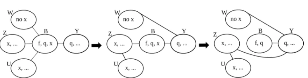
In the following we define two transformation rules which take a tree-decomposition (T, X ) of a graph G, and computes another one without increasing the width nor the size.
Leaf. Let X ∈ X and NT(X) = {X1, · · · , Xd}. Assume that, for any 1 < i ≤
d, Xi ∩ X ⊆ X1. Let (T∗, X∗) = Leaf (X, X1, (T, X )) denote the
tree-decomposition of G obtained by replacing each edge XiX ∈ E(T ) by an edge
XiX1for any 1 < i ≤ d. Note that X becomes a leaf-bag after the operation.
See in Figure 4.
Reduce. Let XX0 ∈ E(T ) with X ⊆ X0. Let (T∗, X∗) = Reduce(X, X0, (T, X ))
denote the decomposition of G obtained by deleting the bag X from the tree-decomposition Leaf (X, X0, (T, X )). Note that the size of the tree-decomposition is decreased by one after the operation.
From any tree-decomposition of G with width k and size s, it is easy to obtain a reduced tree-decomposition of G with width at most k and size at most s − 1 by applying the Reduce operation if it is possible (i.e., if a bag is contained in another one). In particular, any minimum size tree-decomposition is reduced.
We conclude this section by a general lemma on tree-decompositions. This lemma is known as folklore, we recall it for completness.
Lemma 7. Let (T, X ) be a tree-decomposition of a graph G. Let X ∈ X and v, w ∈ X. If there exists a connected component in G \ X containing a neighbor of v and a neighbor ofw, then there is a neighbor bag of X in (T, X ) containing v and w.
Proof. First, let us note that, for any connected subgraph H of G, the set of bags of T which contain a vertex of H induces a subtree of T (the proof can be done by induction on |V (H)|).
1 X 2 X d X X 1 T 2 T d T 1 X 2 X d X X 1 T 2 T d T
➡
( T, X ) ( T*, X*)Figure 4: In a tree-decomposition (T, X ), NT(X) = {X1, · · · , Xd} and for any 1 < i ≤ d, Xi∩ X ⊆
X1. For 1 ≤ i ≤ d, Ti∪ Xiinduces the subtree containing Xiin T \ {XXi}. We replace each edge
XiX ∈ E(T ) by an edge XiX1 for any 1 < i ≤ d. This gives a tree-decomposition (T∗, X∗) =
Leaf (X, X1, (T , X )). X is a leaf-bag in (T∗, X∗).
Let C be a connected component in G\X containing a neighbor of v and a neighbor of w. Let TC0 be the subtree of T induced by the bags that contain at least a vertex of C. Because no vertices of C are contained in the bag X, then TC0 is a subtree of T \ X.
Let TCbe the connected component of T \ X that contains TC0. Let Y ∈ V (TC) be
the bag of TCwhich is a neighbor of X in T . Let x ∈ N (v) ∩ C be a neighbor of v
in C. Then there exists a bag Z ∈ X in TC containing both x and v. So both X and
Z contain vertex v. Then the bag Y , which is on the path between X and Z in T , also contains v. Similarly, we can prove that w ∈ Y .
Corollary 8. Let (T, X ) be a tree-decomposition of a 2-connected graph G. Let X ∈ X and |X| ≤ 2. Then there is a neighbor bag Y of X in (T, X ) such that X ⊆ Y . Proof. Since G is 2-connected, |V (G)| ≥ 3. So there exist at least another bag except X in X .
If |X| = 1, let X = {v}. Then there is a neighbor bag Y of X containing v, since G is 2-connected and v is adjacent to some vertices in G. If X = 2, let X = {v, w}. Let G1 be any connected component in G \ X. If v is not adjacent to any vertex in
G1, then {w} separates V (G1) from {v}. This contradicts with the assumption that G
is 2-connected. So any connected component in G \ X contains a neighbor of v and a neighbor of w. From Lemma 7, there is a neighbor bag Y of X containing v, w, i.e. X ⊆ Y .
3.2. General approach
In what follows, we present the general approach used to design polynomial-time algorithms to compute minimum-size tree-decompositions of graphs with small treewidth. Our algorithms mainly use the notion of potential-leaf.
Let k ≥ 1 and G = (V, E) be a graph with tw(G) ≤ k. The key idea of our algorithms is to identify a finite complete set of potential-leaves. Then, our algorithms
are recursive: given a graph G and a k-potential-leaf H from the complete set, we compute a minimum-size tree-decomposition of G by adding H to a minimum-size tree-decomposition of a smaller graph.
The next lemmas formalize the above paragraph. Given a graph G = (V, E) and a set S ⊆ V , let GS = G ∪ {uv : u, v ∈ S}.
Lemma 9. Let k ≥ 1 and G = (V, E) be a graph with tw(G) ≤ k. Let B ⊆ V be ak-potential-leaf of G and S ⊂ B be the set of vertices of B that have a neighbor in V \ B. Then sk(G) = sk(GS\ (B \ S)) + 1.
Proof. Let us first prove sk(G) ≤ sk(GS \ (B \ S)) + 1. Suppose that (TS, XS) is
a minimum size tree-decomposition of width at most k of the graph GS \ (B \ S).
Then there exists a bag X ∈ XScontaining S because S induces a clique in the graph
GS\ (B \ S). We add the bag B and make it adjacent to X in the tree-decomposition
(TS, XS). We obtain then a tree-decomposition of width at most k for graph G of size
sk(GS\ (B \ S)) + 1.
Now we prove that sk(G) ≥ sk(GS\ (B \ S)) + 1. Let (T, X ) be a minimum size
tree-decomposition of G of width at most k such that B is a leaf bag in (T, X ) . Note that, if B = V then GS\ (B \ S) is the empty graph. Let us assume that B ⊂ V . Then
(T, X ) is also a tree-decomposition of GS. Let B be adjacent to the bag Y in (T, X ).
Then S ⊂ Y since each vertex in S is contained in another bag in (T, X ). Let (T0, X0) be the tree-decomposition obtained by deleting the vertices in B \ S in all the bags of (T, X ). Then B is changed to B0 = S ∈ X0and let Y be changed to Y0∈ X0. So B0 ⊆
Y0. Then the tree-decomposition Reduce(B0, Y0, (T0, X0)) is a tree-decomposition of GS\ (B \ S) of size sk(G) − 1. So sk(G) − 1 ≥ sk(GS\ (B \ S)).
This lemma implies the following corollary:
Corollary 10. Let k ∈ N∗ andC be the class of graphs with treewidth at most k. If there is ag(n)-time algorithm Ak that, for anyn-vertex-graph G ∈ C, computes a
k-potential-leaf of G. Then sk can be computed inO(g(n) · n) time in the class of
n-vertex graphs in C. Moreover, a minimum size tree-decomposition of width at most k can be constructed in the same time.
Proof. Let G ∈ C be a n-vertex-graph. Let us apply Algorithm Akto find a subgraph
H of G in g(n) time, which is a k-potential-leaf of G. Let S ⊂ V (H) be the set of vertices having a neighbor in G \ H and G0= GS\ (V (H) \ S). Then, by Lemma 9,
sk(G) = sk(G0)+1. Finally, |V (G0)| ≤ n−1 and G0has treewidth at most k. We then
proceed recursively. So the total time complexity is O(g(n) · n). Moreover, for any minimum size (sk(G0)) tree-decomposition (T0, X0) of G0of width k, there is a bag X
containing S since S induces a clique in G0. Add a new bag N = V (H) adjacent to X in (T0, X0). The obtained tree-decomposition is a minimum size (s
k(G) = sk(G0) + 1)
tree-decomposition of G of width at most k.
4. Graphs with treewidth at most 2
In this section, we describe the algorithm A2 which computes a 2-potential-leaf
most 2, i.e. partial 2-trees. Please see a complete set of 2-potential-leaves of graphs of treewidth at most 2 in Figure 5. We are going to prove that any of the subgraphs in Figure 5 is a 2-potential-leaf and then that each non-empty graph of treewidth at most 2 contains one of them as a 2-potential-leaf.
Figure 5: Complete set of 2-potential-leaves of graphs of treewidth at most 2.
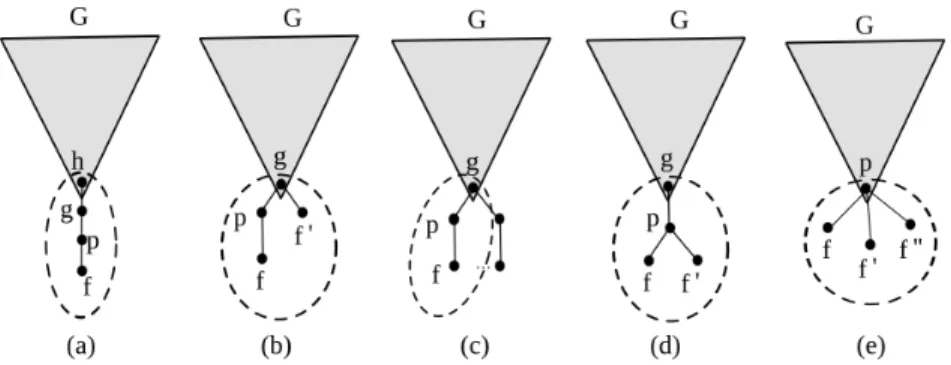
Lemma 11. Let G be a graph with treewidth at most 2 and p ∈ V (G) such that N (p) = {f, q} and f has degree one (see Figure 5(a)). Then {f, p, q} is a 2-potential-leaf ofG.
Proof. Let (T, X ) be any tree-decomposition of G with width at most 2 and size at most s ≥ 1. We show how to modify (T, X ) to obtain a tree-decomposition with width at most 2 and size at most s and in which {f, p, q} is a leaf bag.
Since f p ∈ E(G), there is a bag B in (T, X ) containing both f and p. We may assume that B is the single bag containing f (otherwise, we delete f from any other bag). Similarly, since pq ∈ E(G), let X be a bag in (T, X ) containing both p and q.
First, let us assume that X = B = {f, p, q}. In this case, we may assume that X is the single bag containing p (otherwise, we delete p from any other bag). If X is a leaf bag, then the lemma is proved. Otherwise, let X1, · · · , Xdbe the neighbors of X
in T . Since f and p appear only in X, then X ∩ Xi⊆ {q} for any 1 ≤ i ≤ d. If there
is 1 ≤ i ≤ d such that q ∈ Xi, let us assume w.l.o.g., that q ∈ X1. By definition of
the operation Leaf , the tree-decomposition Leaf (X, X1, (T, X )) has width at most 2
and the same size as (T, X ), and X is a leaf.
Second, consider the case when X 6= B. There are two cases to consider. Either B = {f, p} or B = {f, p, x} with x 6= q. In the latter case, note that there is another bag B0, neighbor of B, that contains x unless x is an isolated vertex of G. In the former case or if x appears only in B (in which case, x is an isolated vertex), let B0 be any neighbor of B. Let (T0, X0) be obtained by deleting f, p in all bags of (T, X ). Then, we contract the edge BB0in T0, i.e., we remove B and make any neighbor of B adjacent to B0. Note that, in the resulting tree-decomposition of G \ {f, p}, there is a bag X0containing q and with |X0| ≤ 2 (the bag that results from X). Finally, we add a bag {f, p, q} adjacent to X0and, if node x was only in B, then we add x to X0. The result is the desired tree-decomposition.
Lemma 12. Let G be a graph with treewidth at most 2 and q ∈ V (G) such that q has at least two one-degree neighborsf and p (see Figure 5(b)). Then {f, p, q} is a 2-potential-leaf ofG.
Proof. Let (T, X ) be any tree-decomposition of G with width at most 2 and size at most s ≥ 1. We show how to modify (T, X ) to obtain a tree-decomposition with width at most 2 and size at most s and in which {f, p, q} is a leaf bag.
Since f q ∈ E(G), there is a bag B in (T, X ) containing both f and q. We may assume that B is the single bag containing f (otherwise, we delete f from any other bag). Similarly, since pq ∈ E(G), let X be a bag in (T, X ) containing both p and q. Again, we may assume that X is the single bag containing p (otherwise, we delete p from any other bag).
First, let us assume that X = B = {f, p, q}. If X is a leaf bag, then the lemma is proved. Otherwise, let X1, · · · , Xdbe the neighbors of X in T . Since f and p appear
only in X, then X ∩ Xi ⊆ {q} for any 1 ≤ i ≤ d. If there is 1 ≤ i ≤ d such that
q ∈ Xi, let us assume w.l.o.g., that q ∈ X1. By definition of the operation Leaf , the
tree-decomposition Leaf (X, X1, (T, X )) has width at most 2, and the same size as
(T, X ), and X is a leaf.
Second, let us assume that X = {f, q} or B = {p, q}. In the former case, we remove p from any bag and add p to X. In the latter case, we remove f from any bag and add f to B. In both cases, we obtain a bag {f, p, q} as in the first case.
Otherwise, let B = {f, q, x}, x 6= p, and X = {p, q, y}, y 6= f .
• If B and X are adjacent in T , then we add a new bag N = {q, x, y}, remove B and X and make each of their neighbors adjacent to the new bag N and, finally, add a leaf-bag {f, p, q} adjacent to N . see Figure 6a. The obtained tree-decomposition has the desired properties.
• Otherwise, if there is a neighbor B0 of B with q, x ∈ B0, then we remove B,
make all neighbors of B adjacent to B0and finally add a leaf-bag {f, p, q} adja-cent to X. The obtained tree-decomposition has the desired properties.
• Otherwise, let B0 be the neighbor of B on the path between B and X. In this
case, q ∈ B0and x /∈ B0. Moreover, q does not belong to any neighbor of B that
contains x and the other way around. For any neighbor Y of B with q ∈ Y (and hence x /∈ Y ), we replace the edge Y B ∈ E(T ) with the edge Y B0. Finally, we
replace the edge BB0∈ E(T ) by the edge BX. See Figure 6b. In the resulting tree-decomposition of G, B and X are adjacent and we are back to the first case.
Lemma 13. Let G be a graph with treewidth at most 2 and q ∈ V (G) such that q has one neighborf with degree 1 and for any vertex w ∈ N (q) \ {f }, {w, q} belongs to a 2-connected component ofG.
IfG has an isolated vertex α, then {q, f, α} is a 2-potential-leaf; otherwise {q, f } is a2-potential-leaf (see Figure 5(c)).
Proof. Let (T, X ) be any tree-decomposition of G with width at most 2 and size at most s ≥ 1. We show how to modify (T, X ) to obtain a tree-decomposition with width at most 2 and size at most s and in which {f, q, α} is a leaf bag if G has an isolated vertex α; and {f, q} is a leaf bag otherwise.
(a) In the tree-decomposition (T, X ), let T1∪ B (resp. T2∪ X) induce the subtree
containing B (resp. X) in T \ {X} (resp. T \ {B}) . We delete B and X, make each of their neighbors adjacent to the new bag N = {q, x, y}, and add a leaf-bag {f, p, q} adjacent to N .
(b) For the sake of simplicity, we show only the induced path from B to X in T and two neighbors Y, Z 6= B0of B. Y contains q and Z contains x. Then we just make Y adjacent to B0 instead of B and make B adjacent to X instead of B0.
Figure 6: Examples illustrating the proof of Lemma 12.
Since f q ∈ E(G), there is a bag B in (T, X ) containing both f and q. We assume that B is the single bag containing f (otherwise, delete f from any other bag).
1. If B = {f, q}, then the intersection of B and any of its neighbor in T is empty or {q}. If there is a neighbor of B containing q, then let X be such a neigh-bor; otherwise let X be any neighbor of B. By definition of the operation Leaf , the tree-decomposition Leaf (B, X, (T, X )) has width at most 2, same size as (T, X ), and B is a leaf. If there are no isolated vertices, we are done. Otherwise, if there is an isolated vertex α in G, then we delete α in all bags of the tree-decomposition Leaf (B, X, (T, X )) and add α to bag B, i.e. make B = {f, p, α}. The result is the desired tree-decomposition.
2. Otherwise let B = {f, q, x}.
(a) If x is a neighbor of q, then x and q are in a 2-connected component of G. So there exists a connected component in G\B containing a vertex adjacent to x and a vertex adjacent to q. From Lemma 7, there is a neighbor X of B in (T, X ) containing both x and q. By definition of the operation Leaf , the tree-decomposition Leaf (B, X, (T, X )) has width at most 2, same size as (T, X ), and B is a leaf. Then we delete x in B, i.e. B = {f, q}. Finally, if α is an isolated vertex of G, we remove it from any other bag and add it to B. The result is the desired tree-decomposition.
(b) Suppose that x is not adjacent to q. If there is a neighbor X of B in (T, X ) containing both x and q, then (T, X ) is modified as in case 2a. Otherwise, any neighbor of B in (T, X ) contains at most one of the vertices q and x. If there is a neighbor of B in T containing q, then let Y be such a neighbor of B; otherwise let Y be any neighbor of B. We delete the edges between
B and all its neighbors not containing x except Y in (T, X ) and make them adjacent to Y .
If there is no neighbor of B containing x, then x is an isolated vertex and we obtain a tree-decomposition of the same size and width as (T, X ), in which there is a leaf bag B = {f, q, x}. It is a required tree-decomposition. Otherwise, let Z be a neighbor of B in (T, X ) containing x, then we delete the edges between B and all its neighbors containing x except Z in (T, X ) and make them adjacent to Z. Now B has only two neighbors Y and Z and B ∩ Y ⊆ {q}, B ∩ Z = {x} and Y ∩ Z = ∅. We delete the edge between B and Z and make Z adjacent to Y . We delete x in B, i.e. make B = {f, q}. See the transformations in Figure 7. Then we obtain a tree-decomposition of the same size and width as (T, X ), in which B = {f, q} is a leaf bag. Again, if α is an isolated vertex of G, we remove it from any other bag and add it to B. The result is the desired tree-decomposition.
Figure 7: To the sake of simplicity, we show only the subtree induced by B, Y and three neighbors Z, W, U of B. Y contains q; Z, U both contain x and W does not contain x. First we make the bag not containing x, e.g. W adjacent to Y instead of B; and make the bag containing x except Z, e.g. U adjacent to Z instead of B. Second, we make Z adjacent to Y instead of B and delete x in B. Then B = {f, q} is a leaf-bag.
Lemma 14. Let G be a graph of treewidth at most 2. Let b ∈ V (G) with N (b) = {a, c}. If N (a) = {b, c} (see Figure 5(d)) or if there is a path, with at least one internal vertex, betweena and c in G \ {b} (see Figure 5(e)), then {a, b, c} is a 2-potential-leaf ofG.
Proof. Let G = (V, E) be a graph of treewidth at most 2. Let b ∈ V with exactly 2 neighbors a, c ∈ V satisfying the hypotheses of the lemma. If V = {a, b, c}, the result holds trivially, so let us assume that |V | ≥ 4.
Let (T, X ) be a reduced tree-decomposition of width at most 2 of G. From (T, X ), we will compute a tree-decomposition (T∗, X∗) of G without increasing the width nor the size and such that {a, b, c} is a leaf-bag of (T∗, X∗).
Let X be any bag of (T, X ) containing {a, b} and Y be any bag containing {b, c}. The bags X, Y exist because ab, bc ∈ E. If X = {a, b}, then there exists a connected component in G \ X containing a neighbor of a and a neighbor of b. By Lemma 7, there is a neighbor of X in (T, X ) that contains both a and b, contradicting the fact that (T, X ) is reduced. So |X| = 3 and, similarly, |Y | = 3.
• Let us first assume that X = Y = {a, b, c}. In particular, it is the case when N (a) = {b, c} since {a, b, c} induces a clique. We may assume that b only belongs to bag X (otherwise, we remove b from any other bag).
If N (a) = {b, c}, then we can also assume that a only belongs to X. Let Z be any neighbor of B containing c if it exists; otherwise let Z be any neighbor of B (Z exists since |V | ≥ 4).
Otherwise, there exists a path P between a and c in G \ {b} with at least one internal vertex. In this latter case, there exists a connected component in G \ X containing a neighbor of a and a neighbor of c. So by Lemma 7, there is a neighbor bag Z of X in (T, X ) containing both a and c. In both cases, Leaf (X, Z, (T, X )) is the desired tree-decomposition.
• X = {a, b, x} and Y = {b, c, y} with x 6= c and y 6= a; and there exists a path P between a and c in G \ {b} with at least one internal vertex. Let Q be the path between X and Y in (T, X ). We may assume that b only belongs to the bags in Q, because otherwise b can be removed from any other bag.
– If X is adjacent to Y , then by properties of tree-decomposition, X ∩ Y separates a and c. Since {b} does not separate a and c, X ∩ Y = {b, x}, i.e. x = y. In this case, (T∗, X∗) is obtained by making X = {a, c, x}
and removing Y from (T, X ), then making all neighbors of Y adjacent to X and finally, adding a bag {a, b, c} adjacent to X.
– Otherwise, let X0be the bag in the path Q containing a, which is closest to Y . Similarly, let Y0be the bag in the path Q containing c, which is closest to X. Finally, let Q0be the path from X0to Y0in T and note that b belongs to each bag in Q0and a and c do not belong to any internal bag in Q0. Also we may assume that b only belongs to the bags in Q0, because otherwise b can be removed from any other bag.
If X0and Y0 are adjacent in T , the proof is similar to the one in previous item. Otherwise, let Z be the neighbor of X0in Q0. By properties of tree-decompositions, X0∩ Z separates a and c. Since {b} does not separate a and c, let X0∩ Z = {b, x0}. Since Z 6= {b, x0} because (T, X ) is reduced,
then Z = {b, x0, z} for some z ∈ V . We replace b with a in all the bags. By doing this (T, X ) is changed to a tree-decomposition (Tc, Xc) of the graph G/ab obtained by contracting the edge ab in G. In (Tc, Xc), the bag X0has
become Xc= {a, x0} and Z is changed to be Zc = {a, x0, z}. So Xccan
be reduced in (Tc, Xc). Moreover Y is changed to Yc = {a, c, y}. To
con-clude, let us add the bag {a, b, c} adjacent to Ycin the tree-decomposition
Reduce(Xc, Zc, (Tc, Xc)). see Figure 8. The result is the desired
tree-decomposition (T∗, X∗) of G.
Before going further, let us introduce some notations. A bridge in a graph G = (V, E) is any subgraph induced by two adjacent vertices u and v of G (i.e., uv ∈ E) such that the number of connected components strictly increases when deleting the
Figure 8: For the sake of simplicity, we show only the path from X to Y . After the two transformations, {a, b, c} is a leaf-bag.
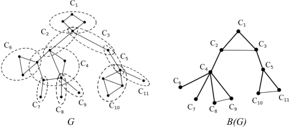
edge uv, but not the two vertices u, v in G, i.e., G0= (V, E \ {uv}) has strictly more connected components than G. A vertex v ∈ V is a cut vertex if {v} is a separator in G. A maximal connected subgraph without a cut vertex is called a block. Thus, every block of a graph G = (V, E) is either a 2-connected component of G or a bridge or an isolated vertex. Conversely, every such subgraph is a block. Different blocks of G intersect in at most one vertex, which is a cut vertex of G. Hence, every edge of G lies in a unique block, and G is the union of its blocks.
Let G = (V, E) be a connected graph and let r ∈ V . A spanning tree T of G is a BFS-tree of G if for any v ∈ V (G), the distance from r to v in G is the same as the one in T . Let B = {C : C is a block of G}. The block graph of G is the graph B(G) whose vertices are the blocks of G and two block-vertices of B(G) are adjacent if the corresponding blocks intersect, that is, B(G) = (B, {C1C2 : C1, C2 ∈ B and
C1∩C26= ∅}). Note that B(G) is connected. Finally, a block-tree of G is any BFS-tree
F (with any arbitrary root) of B(G). See an example in Figure 9.
1 C 2 C 3 C 5 C 4 C 6 C 7 C 8 C 9 C 10 C 11 C 1 C 2 C 3 C 4 C C5 6 C 7 C 8 C C9 10 C C11
G
B(G)
Figure 9: Graph G is connected. For i = 1, . . . , 11, each Ciis a block of G. B(G) is the block graph of
There is a linear (in the number of edges) algorithm for computing all blocks in a given graph [11]. Also a BFS-tree can be found in linear (in the number of vertices plus the number of edges) time. So given a graph G = (V, E), we can compute a block tree F of G in O(|V | + |E|) time.
Now we are ready to prove the next theorem by using the Lemmas 11-14.
Theorem 15. There is an algorithm that, for any n-vertex-m-edge-graph G with treewidth at most2, computes a 2-potential-leaf of G in time O(n + m).
Proof. If n ≤ 3, then V (G) is a 2-potential-leaf of G. Let us assume that n ≥ 4. First, let us compute the set of isolated vertices in G, which can be done in O(n) time. If G has only isolated vertices, then any three vertices induce a 2-potential-leaf of G. Otherwise, there is at least one edge in G.
Let G1be any connected component of G containing at least one edge. If |V (G1)| =
2, then from Lemma 14, either G has an isolated vertex α and {α, u, v} is a 2-potential-leaf or {u, v} is a 2-potential 2-potential-leaf.
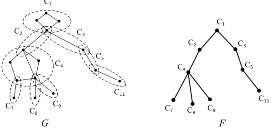
Otherwise, |V (G1)| ≥ 3. We compute a block tree F of G1rooted in an arbitrary
block R. This can be done in time O(n + m). Note that any node in F corresponds to either a 2-connected component of G or a bridge uv ∈ E(G). Let C be a leaf block in F , which is furthest from R and |V (C)| is maximum. There are several cases to be considered. 1 C 2 C 3 C 5 C 4 C 7 C 8 C 9 C 11 C 1 C 2 C 3 C 4 C C5 7 C 8 C C9 11 C
G
F
Figure 10: This graph G is an induced subgraph of the graph in Figure 9. Its block tree F , with root C1, has two blocks less than the one in Figure 9 (the blocks C6and C10). Each one of the leaf blocks,
C7, C8, C9, C11, in F contains two vertices of G.
• let us first assume that C is a bridge in G, i.e. C consists of one edge f p ∈ E(G) and p is a cut vertex. Then f has degree one in G because C is a leaf block in F . Let P be the parent block of C in F . Then any child block A of P in F consists of one edge because C has the maximum number of vertices among all the children of P ; and A is a leaf block in F because C is a furthest leaf from the root block R.
If P has another child block except C in F containing the cut vertex p, then this child block also consists of one edge f0p ∈ E(G), where f0has degree one in G
because this child is also a leaf block in F . For example, in Figure 10, we take C as C8, which intersects C9with a cut vertex. From Lemma 12, {f, p, f0} is a
2-potential-leaf.
Otherwise, P has only one child block C in F containing the cut vertex p. Then any vertex in NG(p)\{f } belongs to P . If P is also a bridge in G, i.e., P consists
of one edge pq ∈ E(G), then p has degree 2 in G. (For example, in Figure 10, take C as C11, whose parent C5is also a bridge in G.) From Lemma 11, {f, p, q}
is a 2-potential-leaf of G. Otherwise, P is a 2-connected component of G and p ∈ V (G) satisfies the hypothesis of Lemma 13. For example, in Figure 10, we take C as C7, whose parent C4 is a 2-connected component of G. Hence,
either G has an isolated vertex α and {α, f, p} is a 2-potential-leaf or {f, p} is a 2-potential-leaf.
• Finally, let us assume that C is a 2-connected component of G. It is known that any graph with at least two vertices of treewidth k contains at least two vertices of degrees at most k [5]. There is no degree one vertex in C because C is 2-connected. So there exists two vertices with degree 2 in C. Since C is a leaf in F , there is only one cut vertex of G in C. So there exists a vertex b in C which has degree two in G. If |V (C)| ≥ 4, then there exists a path between two neighbors a, c of b in G\{b} containing at least one internal vertex. For example, in Figure 9, we take C as C10. From Lemma 14, {a, b, c} is a 2-potential-leaf.
Otherwise C is a triangle {a, b, c} with at least two vertices with degree 2 in G. Again from Lemma 14, {a, b, c} is a 2-potential-leaf.
So the total time complexity is O(n + m).
Corollary 16. s2can be computed in polynomial-time in general graphs. Moreover,
a minimum size tree-decomposition can be constructed in polynomial-time in the class of partial 2-trees.
Proof. Let G be any graph. It can be checked in polynomial-time whether tw(G) ≤ 2 (e.g. see [18]). If tw(G) > 2, then s2 = ∞. Otherwise tw(G) ≤ 2, then the result
follows from Theorem 15 and Corollary 10.
5. Minimum-size tree-decompositions of width at most 3
In this section, we present algorithms to compute s3in the class of trees and
2-connected outerplanar graphs.
5.1. Computation ofs3in trees
In this subsection, given a tree G, we show how to find a 3-potential-leaf in G. We characterize a complete set of 3-potential-leaves of trees in Figure 11. We first prove that each of the subgraphs in Figure 11 is a 3-potential-leaf and then that any tree with at least four vertices contains one of them.
Figure 11: Complete set of 3-potential-leaves of trees.
Lemma 17. Let (T, X ) be a tree-decomposition of a tree G. Let X ∈ X and NT(X) =
{X1, . . . , Xd}, d ≥ 1. Suppose that for any 1 ≤ i ≤ d, Xi∩ X ⊆ {x}. Then there is
a tree-decomposition(T0, X0) of G of the same width and size as (T, X ) such that X is a leaf bag.
Proof. If there is a bag Xifor 1 ≤ i ≤ d containing x, then let B be Xi. Otherwise let
B be any neighbor of X. By definition of the operation Leaf , the tree-decomposition Leaf (X, B, (T, X )) is the desired tree-decomposition.
Lemma 18. Let G be a tree rooted at r ∈ V (G). Let f be a leaf in G, p be the parent off and g be the parent of p in G. Let p have degree 2 in G. Let (T, X ) be a tree-decomposition ofG of width at most 3 and size at most s ≥ 1. If there is no bag in(T, X ) containing all of f, p, g, then there is a tree-decomposition (T0, X0) of G of width at most 3 and size at mosts such that {f, p, g} ∈ X0is a leaf bag.
Proof. Since f p ∈ E(G), there is a bag B in (T, X ) containing both f and p. We may assume that B is the single bag containing f (otherwise, we delete f from any other bag). Similarly, since pg ∈ E(G), let X be a bag in (T, X ) containing both p and g. Let P be the path in T from B to X. Then p is contained in all bags on P and we may assume that p is not contained in any other bags (otherwise, we delete p from any other bag). Let B0be the neighbor of B on P . Then {p} ⊆ B ∩ B0. Note that it is possible that B0= X.
If B = {f, p}, then we make all other neighbors of B adjacent to B0 and delete B. We add a bag {f, p, g} adjacent to X. The result is the desired tree-decomposition (T0, X0).
Otherwise, B contains at least one vertex not in {f, p}. If B ∩ B0 = {p}, then {p} separates g from any vertex in B \ {p}. So B \ {p} = {f }, i.e., B = {f, p}. This contradicts the assumption.
So |B ∩ B0| ≥ 2 and let {p, x} ⊆ B ∩ B0. Then we create a bag Z = (B \ {f, p}) ∪
(B0\ {p, x}) (note that x ∈ Z since x ∈ B.) So |Z| ≤ 4. We make Z adjacent to all neighbors of B and all neighbors of B0, delete the two bags B and B0, and delete f, p from all bags. Finally, we add another new bag N = {f, p, g} adjacent to some bag containing g. The obtained tree-decomposition has width at most 3, same size as (T, X ), and a bag N = {f, p, g} as a leaf.
Lemma 19. Let G be a tree rooted at r ∈ V (G) and |V (G)| ≥ 4. Let f be a leaf in G, p be the parent of f and g be the parent of p in G. Suppose that both p and g have degree 2. Leth be the parent of g (see Figure 11(a)), then H = G[{f, p, g, h}] is a 3-potential-leaf ofG.
Proof. Let (T, X ) be any reduced tree-decomposition of width at most 3 and size at most s ≥ 1 of G. We show how to modify (T, X ) to obtain a tree-decomposition with width at most 3 and size at most s and in which {f, p, g, h} is a leaf bag.
From Lemma 18, we can assume that there is a bag B in (T, X ) containing all f, p, g. We may assume that B is the single bag containing f, p (otherwise, we delete f, p from any other bag). Since gh ∈ E(G), let Y be a bag in (T, X ) containing both h and g.
1. If B = Y = {f, p, g, h}, then the intersection of B and any of its neighbor in T is contained in {h}. A desired tree-decomposition can be obtained from Lemma 17.
2. If B = {f, p, g}, then the intersection of B and any of its neighbors in T is contained in {g}. From Lemma 17, there is a tree-decomposition (T0, X0) of the same width and size as the ones of (T, X ) such that B = {f, p, g} is a leaf. Then we delete B in the tree-decomposition Leaf (B, B0, (T, X )) and add a new bag N = {f, p, g, h} adjacent to Y . The obtained tree-decomposition has the desired properties.
3. Otherwise, B = {f, p, g, x} where x 6= h. Then the intersection of B and any of its neighbor in T is contained in {g, x}. Let P be the path in T from B to Y . Then g is contained in all bags on P . Let B0 be the neighbor of B on P . Note that it is possible that B0 = Y . If B ∩ B0 = {g}, then {g} separates h from x. So x ∈ {f, p} i.e. B = {f, p, g}, a contradiction with the assumption. So we have B ∩ B0 = {g, x}. By definition of the operation Leaf , the tree-decomposition Leaf (B, B0, (T, X )) has width at most 3, same size as (T, X ), and B = {f, p, g, x} is a leaf. Then we delete B in the tree-decomposition Leaf (B, B0, (T, X )) and add a new bag N = {f, p, g, h} adjacent to Y . The obtained tree-decomposition has the desired properties since {g, x} ⊆ B0 and {g, h} ⊆ Y .
Lemma 20. Let G be a tree rooted at r ∈ V (G) and |V (G)| ≥ 4. Let f be a leaf in G, p be the parent of f and g be the parent of p in G. If p has degree 2 and g has a child f0, which is a leaf inG (see Figure 11(b)), then H = G[{f, p, g, f0}] is a 3-potential-leaf ofG.
Proof. Let (T, X ) be any reduced tree-decomposition of width at most 3 and size at most s ≥ 1 of G. We show how to modify (T, X ) to obtain a tree-decomposition with width at most 3 and size at most s and in which {f, p, g, f0} is a leaf bag.
From Lemma 18, we can assume that there is a bag B in (T, X ) containing all of the vertices f, p, g. We may assume that B is the only bag containing f, p (otherwise, we
delete f, p from any other bag). Since gf0∈ E(G), let Y be a bag in (T, X ) containing both f and g. We may assume that Y is the single bag containing f0 (otherwise, we delete f0from any other bag).
• If B = Y = {f, p, g, f0}, then the intersection of B and any of its neighbors
in T is contained in {g}. A desired tree-decomposition can be obtained from Lemma 17.
• If B = {f, p, g}, then we delete f0 in Y and add f0in B; we will be back then to the previous case.
• Otherwise, B = {f, p, g, x} where x 6= f0. The intersection of B and any of its neighbors in T is contained in {g, x}. Let P be the path in T from B to Y . Then g is contained in all bags on P . Let B0 be the neighbor of B on P . If B ∩ B0 = {g, x}, then by definition of the operation Leaf , the tree-decomposition Leaf (B, B0, (T, X )) has width at most 3, same size as (T, X ), and B = {f, p, g, x} is a leaf. In the tree-decomposition Leaf (B, B0, (T, X )), we delete f0in Y , remove x from B, and add f0to B, i.e. make B = {f, p, g, f0}. The obtained tree-decomposition has the desired properties since {g, x} ⊆ B0. Otherwise, if B ∩ B0 = {g}. We delete f0from the bag Y , add x to Y , delete x from B, and add f0 in B, i.e., make B = {f, p, g, f0}. Finally, we make all neighbors of B except B0adjacent to Y since now {g, x} ⊆ Y . The result is the desired tree-decomposition.
Lemma 21. Let G be a tree rooted at r ∈ V (G) and |V (G)| ≥ 3. Let f be one of the furthest leaves fromr, p be the parent of f and g be the parent of p in G. If g has degree at least 3 and any child ofg has degree 2 in G (see Figure 11(c)), then H = G[{f, p, g}] is a 3-potential-leaf of G.
Proof. Let (T, X ) be any reduced tree-decomposition of width at most 3 and size at most s ≥ 1 of G. We show how to modify (T, X ) to obtain a tree-decomposition with width at most 3 and size at most s, and in which {f, p, g, f0} is a leaf bag.
From Lemma 18, we can assume that there is a bag B in (T, X ) containing all the vertices f, p, g. We may assume that B is the only bag containing f, p (otherwise, we delete f, p from any other bag).
1. If B = {f, p, g}, then the intersection of B and any of its neighbors in T is con-tained in {g}. The desired tree-decomposition can be obcon-tained from Lemma 17.
2. Otherwise, B = {f, p, g, x}. In this case, the intersection of B and any of its neighbors in T is contained in {g, x}.
(a) If there is a neighbor B0 of B such that B ∩ B0 = {g, x}, then by defini-tion of the operadefini-tion Leaf , the tree-decomposidefini-tion Leaf (B, B0, (T, X )) has width at most 3, same size as (T, X ), and B = {f, p, g, x} is a leaf. We delete x in B in the tree-decomposition Leaf (B, B0, (T, X )) since {g, x} ⊆ B0. The obtained tree-decomposition has the desired properties.
(b) Otherwise any neighbor of B contains at most one of the vertices g and x. If x is not adjacent to g, then there is a connected component in G \ B containing a neighbor of g and a neighbor of x. From Lemma 7, there exists a neighbor bag of B in (T, X ) containing g and x. This is a contradiction and x is hence adjacent to g in this case.
i. x is a child of g. Then x has exactly one child y, which is a leaf in G since f is one of the furthest leaves from r. Since yx ∈ E(G), there is a bag Y in (T, X ) containing both y and x. We may assume that Y is the only bag containing y (otherwise, we delete y from any other bag). Since {g, x} ⊂ B and any neighbor of B contains at most one of the vertices g and x, any bag except B contains at most one of the vertices g and x. Then g /∈ Y because x ∈ Y . The vertices y, x, g are hence not contained in one bag. From Lemma 18, we can modify (T, X ) to obtain a tree-decomposition (T0, X0) of width at most 3 and size at most s having a leaf bag X = {y, x, g}. Note that x (resp. y) plays the same role as p (resp. f ) in G, i.e., g, p, f and g, x, y are symmetric in G. Hence, the result is the desired tree-decomposition.
ii. x is the parent of g. Let p0be another child of g and let f0be the child of p0, which is a leaf in G. Let B0 be the bag in (T, X ) containing both f0 and p0. We may assume that B0 is the only bag containing f0 (otherwise, we delete f0 from any other bag). Let X0 be a bag
containing both p0 and g. Then we have X0 6= B (because p0 ∈ B)./ Since g ∈ X0, any bag except B contains at most one of the vertices g and x, we have x /∈ X0. In the following, we modify (T, X ) to obtain
a tree-decomposition (T0, X0) with width at most 3 and size at most s having a bag {f0, p0, g}. We will be back then to case 1, since g, p, f and g, p0, f0are symmetric in G.
If B0= X0 = {f0, p0, g} then, we are done. If B0= X0= {f0, p0, g, x0}. Then x06= x, which is the parent of g, since x /∈ X0. So we can do as
in case 2a or case 2(b)i.
Otherwise, B0 6= X0. From Lemma 18, we can modify (T, X ) to
obtain a tree-decomposition with width at most 3 and size at most s having a leaf bag {f0, p0, g}.
Lemma 22. Let G be a tree rooted at r ∈ V (G) and |V (G)| ≥ 4. Let f a leaf in G, p be the parent of f , and g be the parent of p. If p has exactly two children f, f0 inG (see Figure 11(d)), thenH = G[{f, f0, p, g}] is a 3-potential-leaf of G.
Proof. Let (T, X ) be any reduced tree-decomposition of width at most 3 and size at most s ≥ 1 of G. We show how to modify (T, X ) to obtain a tree-decomposition with width at most 3 and size at most s and in which {f, f0, p, g} is a leaf bag.
Since f p ∈ E(G), there is a bag B in (T, X ) containing both f and p. We may assume that B is the only bag containing f (otherwise, we delete f from any other bag). Similarly, let B0be the only bag in (T, X ) containing both f0and p. Let X be a bag containing both p and g.
1. If B = B0 = X = {f, f0, p, g}, then we can assume that B is the only bag containing p (otherwise, we delete p from any other bag). The intersection of B and any of its neighbor in T is contained in {g}. The desired tree-decomposition can then be obtained from Lemma 17.
2. If B = B0 = {f, f0, p}, then the intersection of B and any of its neighbors in T
is contained in {p}. Let Y be a neighbor of B in T containing p. By definition of the operation Leaf , the tree-decomposition Leaf (B, Y, (T, X )) has width at most 3, same size as (T, X ), and B = {f, f0, p} is a leaf. We delete B and add a new bag N = {f, f0, p, g} adjacent to X. The result is the desired tree-decomposition.
3. If B = B0 = {f, f0, p, x} and x 6= g, then the intersection of B and any of its neighbors in T is contained in {p, x}. Since x /∈ {f, f0, g}, p is not adjacent
to x. There is a connected component in G \ B containing a neighbor of p and a neighbor of x. From Lemma 7, there exists a neighbor bag of B in (T, X ) containing p and x. Let Y be such a neighbor of B in T . By definition of the operation Leaf , the tree-decomposition Leaf (B, Y, (T, X )) has width at most 3, same size as (T, X ), and B = {f, f0, p, x} is a leaf. We delete x from B and obtain a tree-decomposition having a bag {f, f0, p}. We will be back then to case 2.
4. If B 6= B0 and |B| ≤ 3, then we delete f0from B and add f0to B. We will be back then to case 2 or 3. The proof is similar if B 6= B0and |B0| ≤ 3.
5. Otherwise, if B 6= B0 and |B| = |B0| = 4, let B = {f, p, x, y} and B0 =
{f0, p, x0, y0}. Let P be the path in T from B to B0. Then p is contained in all
bags on P . Let Y be the neighbor of B on P . If B ∩Y = {p}, then {p} separates x from x0. But p is not a separator for any two vertices in V (G) \ {f, f0}. This is a contradiction. So w.l.o.g. we can assume that B ∩ Y ⊇ {p, x}. We delete f, f0, p in all bags of (T, X ), add a new bag Z = {x, y} ∪ Y \ {p, x} adjacent to all neighbors of the two bags B, Y and delete B and Y . Finally, we add another new bag N = {f, f0, p, g} adjacent to a bag containing g. The obtained tree-decomposition has the desired properties.
Lemma 23. Let G be a tree rooted at r ∈ V (G) and |V (G)| ≥ 4. Let all children of p be leaves in G and p have at least three children f, f0, f00(see Figure 11(e)). Then H = G[{p, f, f0, f00}] is a 3-potential-leaf of G.
Proof. Let (T, X ) be any reduced tree-decomposition of width at most 3 and size at most s ≥ 1 of G. We show how to modify (T, X ) to obtain a tree-decomposition with width at most 3 and size at most s and in which {p, f, f0, f00} is a leaf bag.
Since f p ∈ E(G), there is a bag B in (T, X ) containing both f and p. We may assume that B is the only bag containing f (otherwise, we delete f from any other bag). Similarly, let B0 (resp. B00) be the only bag in (T, X ) containing both f0 (resp. f0) and p.
1. If B = B0 = B00 = {f, f0, f00, p}, then the intersection of B and any of its neighbors in T is contained in {p}. A desired tree-decomposition can be ob-tained from Lemma 17.
2. If B = B0 = {f, f0, p}, then we delete f00 from B00 and add f00 to B. We will be back then to case 1. The proof is similar for B = B00 = {f, f00, p} or
B0= B00= {f0, f00, p}.
3. If B = B0 = {f, f0, p, x} and x 6= f00, then the intersection of B and any of its neighbors in T is contained in {p, x}. If x is a child of p, then x is also a leaf in G and x play the same role as f00. We are then in case 1. Therefore, in the following we assume that x is not a child of p.
If x is not the parent of p, then p is not adjacent to x. So there is a con-nected component in G \ B containing a neighbor of p and a neighbor of x. From Lemma 7, there exists a neighbor bag of B in (T, X ) containing p and x. Let Y be such a neighbor of B in T . By definition of the operation Leaf , the tree-decomposition Leaf (B, Y, (T, X )) has width at most 3, same size as (T, X ), and B = {f, f0, p, x} is a leaf. We delete x from B and obtain a tree-decomposition having a bag {f, f0, p}. We are back then to case 2.
Otherwise, if x is the parent of p, let P be the path in T from B to B00. Then p is contained in all bags on P . Let Y be the neighbor of B on P . If B ∩ Y = {p, x}, then by definition of the operation Leaf , the tree-decomposition Leaf (B, Y, (T, X )) has width at most 3, same size as (T, X ), and B = {f, f0, p, x} is a leaf. By deleting x from B we will be back to case 2. Otherwise, if B ∩ Y = {p}, then {p} separates x from all vertices in B00\ {p}. All ver-tices in B00\ {p} are children of p and so they are leaves in G. We can assume then that any vertex in B00\{p} is contained only in B00(otherwise we can delete
it in any other bag). We delete f, f0from B, add vertices of B00\ {f00, p} in B,
and make B00= {f, f0, f00, p}. We will be back then to case 1.
The cases B = B00 = {f, f00, p, x} and x 6= f0 or B0 = B00 = {f0, f00, p, x} and x 6= f can be proved in a similar way.
4. Otherwise, no two vertices of f, f0, f00are contained in a same bag.
If |B| ≤ 3, then we delete f0in B0 and add f0in B. We will be then in case 2 or 3. The proof is similar if |B0| ≤ 3 or |B00| ≤ 3.
Otherwise |B| = |B0| = |B00| = 4. In the following, we are going to modify (T, X ) to obtain a tree-decomposition with width at most 3 and size at most s having a bag X containing at least two of the vertices f, f0, f00or f ∈ X and |X| ≤ 3. We are then in the above cases. Note that all children of p play the same role (they are all leaves) in G. So it is enough to have that X contains at least two children of p or that X contains one child of p and |X| ≤ 3.
Let Tpbe the subtree in T induced by all the bags containing p. If |V (Tp)| ≤ 2,
there exists one bag containing at least two children of p since p has at least three children. We assume then that |V (Tp)| ≥ 3. There is a bag R ∈ V (Tp)
leaf bags in Tpfrom R. If there is no child of p in L, then we can delete p from
L and consider Tp\ {L}. We can assume then that there is a vertex l ∈ L, which
is a child of p in G. Let Y be the neighbor of L in Tp. If the intersection of
L ∩ Y = {p}, then p separate any vertex in L \ {p} and any vertex in Y \ {p}. So at least one of the bags L, Y contains only p and children of p. We denote this bag by X. Either X contains at least two children of p or X contains only one children and |X| = 2. So (T, X ) and X satisfy the desired properties. Otherwise, |L ∩ Y | ≥ 2. If Y has no other child except L in Tp, then Y 6= R
since |V (Tp)| ≥ 3. Let X = {p, l} if Y contains no child of p and X = {p, l, l0}
if Y contains one child l0 of p. We add a new bag Z = Y ∪ L \ X. Since |Y ∩ L| ≥ 2, we have |Y ∪ L| ≤ 6. Also |Z| ≤ 4, since X ⊆ Y ∪ L and |X| ≥ 2. We make Z adjacent to all neighbors of Y, L in T and delete Y, L. Finally, we make X adjacent to R. The obtained tree-decomposition and X have the desired properties.
Otherwise, Y has at least another child L0in Tp. Then L0 is also a furthest leaf
from R in Tp, since L is a furthest leaf from R. For the same reason as L,
there is a vertex l0 ∈ L, which is a child of p in G. Let L = {l, p, x, y} and L0 = {l0, p, x0, y0}. The intersection of L (resp. L0) and any of its neighbors in T except Y is contained in {x, y} (resp. {x0, y0}). We create a new bag N = {x, y, x0, y0} adjacent to all neighbors of L and L0 and delete L and L0.
Finally, we add another bag X = {p, l, l0} adjacent to Y . The obtained tree-decomposition and X have the desired properties.
From Lemmas 19- 23 and Corollary 10, we obtain the following result.
Corollary 24. s3 and a minimum size tree-decomposition of width at most 3 can be
computed in polynomial-time in the class of trees.
Proof. From Corollary 10, it is enough to prove that we can find a 3-potential-leaf in any tree in polynomial time.
Let G be any tree. If |V (G)| ≤ 4, then V (G) is a 3-potential-leaf. Let us assume that |V (G)| ≥ 5. We root G at any vertex r. Let f be one of the furthest leaves from r in G. Let p, g, h be the first three vertices on the path from f to r in G (if they exist), i.e. p is f ’s parent; g is the parent of p, and h is the parent of g in G.
• If g, p both have only one child in G, then {f, p, g, h} is a 3-potential-leaf of G from Lemma 19;
• If p has only one child and g has a child f0, which is a leaf in G, then {f, p, g, f0}
is a 3-potential-leaf of G from Lemma 20;
• If p has only one child and any child of g has exactly one child, then {f, p, g} is a 3-potential-leaf of G from Lemma 21;
• If p has only one child and there exists a child p0 of g, which has exactly two
• If p has only one child and there exists a child p0 of g, which has at least
three children f1, f2, f3, then {f1, f2, f3, p0} is a 3-potential-leaf of G from
Lemma 23;
• If p has exactly two children f, f0, then {f, f0, p, g} is a 3-potential-leaf of G
from Lemma 22;
• Otherwise, if p has at least three children f, f0, f00, then {f, f0, f00, p} is a 3-potential-leaf of G from Lemma 23.
In fact, the algorithm for trees can be extended to forests by considering their con-nected component, i.e., trees. The only difference is in Lemma 21 the 3-potential-leaf becomes {f, p, g, α} if there is an isolated vertex α in the given forest.
5.2. Computation ofs3in 2-connected outerplanar graphs
In this subsection, given a 2-connected outerplanar graph G, we show how to find a 3-potential-leaf in G. We give in Figure 12 a complete set of 3-potential-leaves of 2-connected outerplanar graphs. We first prove that each subgraph in the Figure 12 is a 3-potential-leaf and then we show that any 2-connected outerplanar graph contains one of them.
Figure 12: Complete set of 3-potential-leaves of 2-connected outerplanar graphs.
The following fact is well known for 2-connected outerplanar graphs.
Lemma 25. [17] A 2-connected outerplanar graph has a unique Hamiltonian cycle.
In the rest of this subsection, let G be a 2-connected outerplanar graph and C be the Hamiltonian cycle in G.
Definition 2. Any edge in E(G) \ E(C) is called a chord in G.
The vertices v1, . . . , vj ∈ V (G), for 2 ≤ j ≤ |V (G)|, are consecutive in C (we

![Figure 2: Examples of gadgets in graph G(S, b) [9]](https://thumb-eu.123doks.com/thumbv2/123doknet/13477652.413103/6.918.211.717.206.303/figure-examples-gadgets-graph-g-s-b.webp)