Perceptual Hysteresis Thresholding:
Towards Driver Visibility Descriptors
Nicolas Hautière, Jean-Philippe Tarel, Roland Brémond
Laboratoire Central des Ponts et Chaussées
58 boulevard Lefebvre, 75732 Paris cedex 15, France
email: {hautiere, tarel, bremond}@lcpc.fr
Abstract
To develop driving assistance systems which alert the driver in case of inadequate speed according to the visi-bility conditions, it is necessary to have descriptors of the driver visibility and in particular to detect the visible fea-tures in the image grabbed by the camera. In this aim, an hysteresis filter is proposed, which is based on the Visibility Level (VL) rather than on the gradient magnitude of edges. First, edges are extracted. Second, to compute the VL of the edges, a threshold function is computed according to the op-tical characteristics of the sensor and a Contrast Sensitivity Function of the Human Visual System. Then, the DCT coef-ficients of each 8× 8 block are computed. For each block, the maximum ratio between a DCT coefficient of the block and the corresponding coefficient of the previous threshold function is computed to determine its VL. Then, hysteresis filter is performed on VL values along edges which leads to a perceptual hysteresis thresholding. Some guidelines to set the thresholds are indicated. Results are given on images grabbed onboard a vehicle. Finally, different techniques to use this hysteresis thresholding in the domain of driving as-sistances are proposed.
1
Introduction
The major part of all the information used in driving is visual [32]. Reduced visibility thus leads to accidents. Re-ductions in visibility may have a variety of causes, namely the geometry of the road scene, the presence of obstacles or adverse weather/lighting conditions. Different proposals exist in the literature to mitigate the dangerousness of each of these situations. Thereafter, these different solutions may be fused to derive intelligent speed adaptation (ISA) sys-tems which take into account the visibility conditions.
The problem of the road geometry is tackled by estimat-ing the geometry visibility range usestimat-ing either a rotative
li-dar coupled with a high-precision GPS [8] or high resolu-tion cameras [6, 33]. A night-visibility index using a ded-icated vehicle to estimate the retroreflection of the road is proposed in [9]. In these applications, the computations are made off-line. By putting these output values on a digital map, the driver may be warned when approaching an area with a low geometrical visibility or a low night-visibility index. One must notice that lane keeping systems may also improve their reliability by exploiting such beforehand ob-tained maps [22, 24]. To reduce the masking of the road infrastructure caused by other vehicles, some specific adap-tive cruise control systems have been developed to maintain the followed vehicles in a small solid angle [20].
The presence of daytime fog and low visibility areas can be detected using in-vehicle cameras [19, 17]. This infor-mation can be used to adapt the operation range of opti-cal sensors and to enhance signal processings [18] or to in-form the driver if he is driving too quickly according to the measured visibility conditions. Because the driver and the camera do not have the same visual performances, it is nec-essary to take into account the mapping function between the driver and camera performances, which includes among other parameters the camera response function [14]. There-after, detecting the visible edges in the image is a critical step to assess the driver visibility. In daytime fog, accord-ing to CIE recommendations [2], the visible edges can be assimilated to the set of edges having a local contrast above 5% [17]. In other cases, the situation is more complicated. In this paper, we propose such a technique based on the Contrast Sensitivity Function (CSF) of the Human Visual System (HVS).
Edges detection is a classical problem in computer vi-sion. Different reviews of work on edges detection are for a long time available in the literature [28, 34]. Gradient mag-nitude [30], zero-crossing [25], optimality criterion [12] are among the most used techniques. However, a problem faced by edges detectors is the choice of relevant threshold values which are often empirically chosen. One of the most ef-fective technique is hysteresis thresholding. However, the
high and the low threshold values constituting the hystere-sis are most of the time both arbitrary selected. In order to automatically find the best threshold, standardizations of gradient magnitudes according to the surrounding pixels have been proposed. In this aim, statistical approaches have been developed [31]. Otherwise, approaches inspired by the HVS characteristics have been tested, e.g. [27, 15]. In our application context, it is straightforward to understand that our proposal belongs to the latter family. Compared to the numerous methods in the literature devoted to biologi-cally inspired edges detection, our method does not aim at fully mimicing the HVS. It aims at introducing some visual mechanisms in image processing techniques. It enables us to develop well-founded algorithms which are also quick enough to be used in driving assistance systems.
We propose a hysteresis thresholding technique whose low and high thresholds are based on Visibility Levels (VL) in reference to [1]. These VLs are based on the CSF of a human eye [11]. Thus, we compute the angular resolution of the device used to grab the pictures using its optical char-acteristics. Then, a Contrast Threshold Function (CTF) is built by taking into account the angular resolution of the sensor and a classical model of CSF. Within each 8 × 8 block of pixels, we compute the maximum ratio between a Discrete Cosine Transform (DCT) coefficient of the block and the corresponding coefficient of the CTF to determine the VL of the block. Using this VL information, a hystere-sis thresholding is applied using predefined low and high thresholds on VLs and is used to select visible edges in nat-ural images from the precomputed edge map. Compared to [15], we do not wish to automatically extract all visible edges and do not mimic the biological structure of the HVS like in [27]. Our aim is rather to select the edges in the im-age according to their perceptual relevance. Thereafter, the properties of the proposed visibility criterion allows to al-ways set the low threshold at 1 and to set the high threshold depending on the aimed application (e.g. 7 for a night-time driving task [3] and at least 20 for a reading task [1]).
Once the visible edges have been extracted, it is then pos-sible to combine them with other algorithms to derive more sophisticated descriptors of the driver visibility.
This paper is organized as follows. First, a geomet-ric camera model is recalled. Then, a model of contrast sensitivity function of the human visual system is summa-rized. Then, the implementation of our visibility criteria is explained. This leads to propose a perceptual hystere-sis thresholding. Some perspectives for validating the pro-posed algorithm from a psychophysical point of view are given. Finally, different solutions to derive descriptors of the driver visibility are briefly presented.
2
Angular Resolution of a Camera
In this section, we express the angular resolution of a CCD camera in cycles per degree (cpd). This unit is used to measure how well details of an object can be seen separately without being blurry. This is the number of lines that can be distinguished in a degree of a visual field.
Figure 1. Geometric camera model to com-pute its angular resolution. Parameters : f focal length, C optical center, θ visual field, d corresponding length on the CCD array.
With the notations of Fig. 1, the length d for a visual field θ = 1o is expressed by d = 2f tanθ
2. To have the maximum angular resolution rcpd∗ of the camera in cpd, it is enough to divide d by the size 2tpixof two pixels (black and white alternation) of the CCD array:
rcpd∗ = f tpix
tanθ
2 (1)
This is a first order approximation as the resolution of the camera is also affected by the diffraction of light against the lens, which leads to a reduced camera resolution when the aperture of the lens decreases. However, the proposed algorithm is less sensitive to this phenomena. This is not the case of the approach described in [15] where the diffraction phenomena must be also taken into account.
3
Human Vision System Modeling
In the previous section, we recall a first order approxi-mation of the angular resolution of a CCD camera. Let’s now consider some characteristics of the HVS.
It is remarkable that our ability to discern low contrast patterns varies with the size of the pattern, that is to say its spatial frequency f , which is often expressed in cpd. The CTF is a measure at a given spatial frequency of the mini-mum contrast needed for an object, in fact a sinusoidal grat-ing, to become visible. This CTF is defined as 1/CSF, where
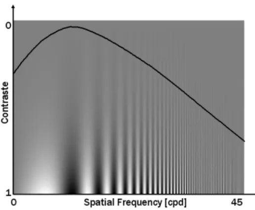
Figure 2. Contrast Sensitivity Function (CSF) of the Human Visual System.
CSF is a Contrast Sensitivity Function (see Fig. 2). Several CSF models have been proposed in the literature [10, 5]. In this paper, we use the widely accepted, at least in the signal processing area, CSF detailed in [23], plotted in Fig. 3 and expressed by:
CSF (f ) = 2.6(0.0192 + 0.114f )e−(0.114f )1.1 (2)
Figure 3. CSF (—) and CTF (– –) of the HVS, proposed by Mannos [23].
4
Design of a Visibility Criteria
In this section, we design a method which computes the VL of a block of pixels. In this aim, we compute the spec-trum of each block and compare each coefficient with the minimum required to be visible by a human eye.
4.1
DCT Transform
We use the DCT to transform the image from the spatial domain to the frequency domain. We denote A = {aij},
a block of the original image and B = {bij}, the corre-sponding block in the DCT transformed image. With these notations, the bijcoefficients are expressed by:
bij= 2 ncicj n−1 X k=0 n−1 X l=0 cos " (2k + 1)iπ 2n # cos " (2l + 1)jπ 2n # akl (3) where c0 = 1/ √
2, ci = 1 for i = 1. . .n-1and n denotes the block width. Following the JPEG format [35], we use n = 8.
Then, to express the DCT coefficients in cycles per de-grees, we simply consider that the maximum frequency fmax of the DCT transform, see (4), expressed in cycles per pixel (cpp), is obtained for the maximum resolution of the sensor, that is to say r∗cpd.
fmax= 4n
2n − 1 (4)
It is interesting to notice that fmaxgoes to 2 cpp as n goes to infinity.
Finally, to express the DCT coefficients {bij} of a block B in cpd and to plot the DCT coefficients of a block with re-spect to the corresponding values of the CTF (see Fig. 5), it is enough to use the scale factor (5) obtained by computing the ratio between (1) and (4):
(2n − 1) 4n f tpix tanθ 2 (5)
Figure 4. Curves of the CSF and of the CTF for the sensor used to grab the samples im-ages given in the paper: tpix = 8.3µm, f = 8.5mm.
In our tests, we use images which have been grabbed by a CCD camera. The reconstructed CSF and CTF for this sensor is plotted in Fig. 4. An important property of this sensor configuration is that the peak of sensitivity of the
HVS is taken into account (see Fig. 3 between 0.5 and 10 for comparison). We used a CCD sensor with short expo-sures. We can thus assume that for this sensor the mapping between luminance and intensity is linear, at least for day-time lighting conditions, which means ∆L ≡ ∆I. This is an important point to remember for the next paragraph.
Figure 5. Computation of VLp in the blocks marked with an arrow under sunny weather and foggy weather. The CTF is plotted in white and the spectrum of the block is rep-resented by the different black peaks: (a)
VLp = 17; (b) VLp < 1; (c) VLp = 4.6; (d) VLp < 1. Only the blocks in (a) and (c) con-tain visible edges according to the definition of VLp.
4.2
Visibility Criteria
For non-periodic targets, visibility can be related to the (Weber) luminance contrast C, which is defined as:
C =∆L Lb
=Lt− Lb Lb
(6) where ∆L is the difference in luminance, between object and background, Ltis the luminance of the target, Lbis the luminance of the background.
The threshold contrast ∆Lthresholdindicates a value at which a target of defined size becomes perceptible with a high probability. Based on Weber’s model or Blackwell’s reference models, this threshold depends on target size and light level, decreasing with increase of light level. For suprathreshold contrasts, i.e. for contrast thresholds above the visibility threshold, the visibility level (VL) of a target
can be quantified by the ratio [1]: VL = Actual contrast
Threshold contrast (7) At threshold, the visibility level equals one and above threshold it is greater than one. Combining (6) and (7), we have:
VL = (∆L/Lb)actual/(∆L/Lb)threshold (8)
As the background luminance Lb is the same for both conditions, then this equation reduces to:
VL = ∆Lactual/∆Lthreshold (9) In any given situation, it is possible to measure the luminance of the target and its background, which gives ∆Lactual but in order to estimate VL, we also need to know the value of ∆Lthreshold. This can be estimated using Adrian’s target visibility model [4] based on experimental data.
By analogy with the definition of VL for non-periodic targets, we propose a new definition of the visibility level, denoted VLp, valid for periodic targets, i.e. gratings. Hence, to obtain the VLpof a block, we first consider the ratio rijbetween a DCT coefficient of the block and the cor-responding coefficient of the CTF model given in section 3:
rij = bij CTFij
(10) Based on the definition of the CSF, it is enough that one of the coefficients rij is greater than 1 to consider that the block of pixels contains visible edges. Therefore, to define VLp, we propose to choose the greatest rij. The proposed expression for VLpis thus:
VLp= max (i,j)6=(0,0)
rij (11)
Based on this definition, if VLp < 1, we can con-sider that the concon-sidered block of pixels contains no visible edges.
First, we illustrate in Fig. 5 the concept in different blocks of images under sunny weather and foggy weather. For each considered image block, the spectrum is plotted with respect to the CTF. VLpvalues are given.
Second, Fig. 6 displays VLp ≥ 1 maps computed on sample images with different lighting conditions (daytime, nighttime with public lighting, daytime fog). The whiter the pixel is, the bigger VLpis.
5
Perceptual Hysteresis Thresholding
5.1
Edges Detection by Segmentation
Although the proposed approach may be used in con-jonction with different edge detectors, like Canny-Deriche’s
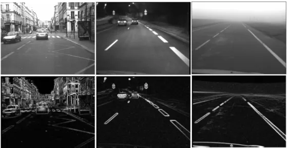
Figure 6. First row: original images (768x576) with different lighting conditions. Second row: VLp≥ 1 maps. The whiter the pixel is, the bigger VLpis.
one [12], zero-crossing approach [25] or Sobel’s approach [30], we propose an alternative method which fits well with our approach and consists in finding the border which max-imizes the contrast between two parts of a block, without adding a threshold on this contrast value. The edges are the pixels on this border. This approach is based on Köhler’s binarization method [21] and is described in [16].
5.2
Hysteresis Thresholding on the
Visi-bility Levels
In the usual hysteresis thresholding, a high threshold and a low threshold are set. In a first pass, all pixels with gra-dient value greater than the high threshold are seeds for edges. In the next pass, any pixels with a gradient greater than the low threshold and adjacent or closely neighboring other edge pixels are also classified as edge pixels. This technique for detecting the edges is inspired by biological mechanisms [13].
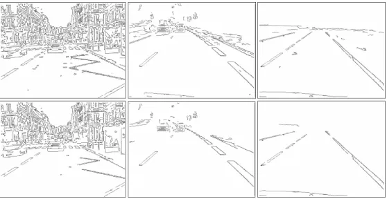
We propose to replace these thresholds on the gradient magnitude by thresholds on the V Lp (cf. Fig. 7) as ex-plained in section 4.2. Thus, the algorithm is as following: first, all possible edges are extracted (see paragraph 5.1), second, the edges are selected thanks to its V Lpvalue using low tL and high tH thresholds. Examples of edges detec-tion are given in Fig. 8 for two sets of thresholds: tL = 1, tH = 10 and (tL = 1, tH = 20. To help visualize the differences between the two sets, the image differences are also shown in Fig. 9. One can notice that even using the first set of thresholds (first row of Fig. 8), no noisy features are detected whatever are the lighting conditions whereas
Figure 7. Principle behind thresholding by hysteresis: points (i,j) are marked by two thresholds. The lower threshold tLgenerates the ”candidate” points. The upper thresh-old tH provides a good indication of the ex-istence of a contour.
Figure 8. Results of edges detection. First row: tL= 1and tH = 10; second row : tL= 1and tH = 20.
thresholds are fixed. The method is thus clearly adaptive.
5.3
Contrast Detection Threshold of the
Human Eye
The value of tLis easy to choose, because it can be re-lated to the HVS. Provided that the proposed analogy is relevant, setting tL = 1 should be appropriate for most applications. The value of tH depends on the application. For lighting engineering, the Commission Internationale de l’Éclairage (CIE) published some recommandations to ade-quately set the Visibility Levels thresholds according to the complexity of the visual task [1]. For example, [3] explains that VL = 7 is a adequate value for night-time driving task. It should be advantageous to set tL = 7 as a starting point. However, a psychophysical validation is necessary (see paragraph 7).
6
Towards Road Visibility Descriptors
Once visible edges have been extracted, they can be used in the context of an onboard camera to derive driver visibil-ity descriptors.First, the range to the most distant visible edge belonging to the road surface can be computed. Using stereovision, the pixels belonging to the road surface can be extracted. Then, by scanning the disparity map from top to bottom starting from the horizon line, the first visible edge which is encountered gives the visibility distance. This process has been already implemented for daytime fog images [17]. If the vehicle has only one camera, edges belonging to the
road plane can also be extracted using successive images alignment [7].
Second, already existing driving assistance systems can be used. In particular, lane markings detectors can be used to derive visibility descriptors, what was pioneered in [29].
7
Future Works
We plan three steps to complete and validate the algo-rithm from a psychophysical point of view.
1. An extension to color images is planned. The idea is take into account the different sensitivities of the HVS to chromatic and achromatic contrasts [36].
2. The CSF is valid for a given adaptation level of the HVS, which is be approximately related to the mean luminance of the scene. In other words, the CSF should not be the same for daily and night scenes. Then, it would be necessary to compare the edges de-tection results according to the chosen CSF. Finally, an interesting additional step would be to automatically select the properly CSF according to the image con-text.
3. To validate the approach, we propose to compare our results with the set of edges which are manually ex-tracted by different people. This work has been done previously for classical edges detectors [26] and the image databases are available. The results show that none of the approaches give results which resemble the manually extracted edges. The fact that our threshold-ing technique is based on some characteristics of the HVS may lead to better results.
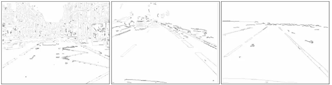
Figure 9. Images of difference between the images of the first and the second row of Fig. 8. Grey: common edges ; black: edges only detected in the first row.
8
Conclusion
In this paper, we present a visible edges selector and use it in the context of in-vehicle applications. It proposes an alternative to the traditional hysteresis filtering which re-lies on low and high thresholds on the gradient magnitude. Thus, we propose to replace them by visibility levels which take into account the spectrum of an image block and com-pare it to the inverse of a contrast sensitivity function of the human visual system. By applying this so called percep-tual hysteresis filtering to edges extracted by any kind of technique, only visible edges are selected. The low thresh-old can be fixed at 1 in general. Some guidelines to set the high threshold are proposed. Approaches to complete and validate the algorithm from a psychophysical point of view are proposed. This algorithm may be used to develop so-phisticated driver visibility descriptors. Thereafter, it can be fused with other visibility descriptors of the road geome-try, the night-visibility or the weather conditions to develop driving assistance systems which takes into account all the visibility conditions.
Acknowledgments
This work is partly founded by the French ANR project DIVAS (2007-2010) dealing with vehicle-infrastructure co-operative systems.
References
[1] An Analytic Model for Describing the Influence of Lighting Parameters Upon Visual Performance, volume 2: Summary and application guidelines. Publication CIE 19, 1981. [2] International lighting vocabulary. Number 17.4.
Commis-sion Internationale de l’Éclairage, 1987.
[3] W. Adrian. Visibility level under nighttime driving con-ditions. Journal of the Illumination Engineering Society, 16(2):3–12, 1987.
[4] W. Adrian. Visibility of targets: model for calculation. Lighting Research and Technologies, 21:181–188, 1989. [5] P. G. J. Barten. Contrast sensitivity of the human eye and its
effects on image quality. SPIE, 1999.
[6] E. Bigorgne and J.-P. Tarel. Backward segmentation and region fitting for geometrical visibility range estimation. In submitted to Asian Conference on Computer Vision, Tokyo, Japan, November 2007.
[7] C. Boussard, N. Hautière, and B. d’Andréa Novel. Vi-sion guided by vehicle dynamics for onboard estimation of the visibility range. In IFAC Symposium on Intelligent Au-tonomous Vehicles, Toulouse, France, September 2007. [8] X. Brun, F. Goulette, P. Charbonnier, C. Bertoncini, and
S. Blaes. Modélisation 3d de routes par télémétrie laser em-barquée pour la mesure de distance de visibilité, 5-6 décem-bre 2006. In Journées des Sciences de l’Ingénieur, Marne la Vallée, France, December 2006.
[9] R. Brémond, H. Choukour, Y. Guillard, and E. Dumont. A night-time road visibility index for the diagnosis of rural road networks. In 26th session of the CIE, Beijing, China, July 2007.
[10] F. W. Campbell and J. G. Robson. Application of fourier analysis to the visibiliy of gratings. The Journal of Physiol-ogy, pages 551–566, 1968.
[11] Committee On Vision. Emergent Techniques for Assessment of Visual Performances. National Academic Press, 1985. [12] R. Deriche. Using canny’s criteria to derive an optimal edge
detector recursively implemented. International Journal on Computer Vision, 2(1), 1987.
[13] J. A. Ferwerda. Elements of early vision for computer graph-ics. IEEE Computer Graphics and Applications, 21(5):22– 33, 2001.
[14] M. Grossberg and S. K. Nayar. Modelling the space of cam-era response functions. IEEE Transactions on Pattern Anal-ysis and Machine Intelligence, 26(10):1272–1282, 2004. [15] N. Hautière and D. Aubert. Visibles Edges Thresholding: a
HVS based Approach. In International Conference on Pat-tern Recognition, volume 2, pages 155–158, August 2006. [16] N. Hautière, D. Aubert, and M. Jourlin. Measurement of
local contrast in images, application to the measurement of visibility distance through use of an onboard camera. Traite-ment du Signal, 23(2):145–158, Septembre 2006.
[17] N. Hautière, R. Labayrade, and D. Aubert. Real-Time Dis-parity Contrast Combination for Onboard Estimation of the Visibility Distance. IEEE Transactions on Intelligent Trans-portation Systems, 7(2):201–212, June 2006.
[18] N. Hautière, J.-P. Tarel, and D. Aubert. Towards fog-free in-vehicle vision systems through contrast restoration. In IEEE Conference on Computer Vision and Pattern Recognition, Minneapolis, USA, June 2007.
[19] N. Hautière, J.-P. Tarel, J. Lavenant, and D. Aubert. Auto-matic Fog Detection and Estimation of Visibility Distance through use of an Onboard Camera. Machine Vision and Applications Journal, 17(1):8–20, April 2006.
[20] H. Kumon, Y. Tamatsu, T. Ogawa, and I. Masaki. ACC in consideration of visibility with sensor fusion technology un-der the concept of TACS. In IEEE Intelligent Vehicles Sym-posium, Tokyo, Japan, June 2005.
[21] R. Köhler. A segmentation system based on threshold-ing. Graphical Models and Image Processing, 15:319–338, 1981.
[22] R. Labayrade. How autonomous mapping can help a road lane detection system? In IEEE International Conference on Control, Automation, Robotics and Vision, Singapore, De-cember 2006.
[23] J. Mannos and D. Sakrison. The effects of visual fidelity criterion on the encoding of images. IEEE Transactions on Information Theory, IT-20(4):525–536, 1974.
[24] T. Manolis, A. Polychronopoulos, and A. Amditis. Using digital maps to enhance lane keeping support systems. In IEEE Intelligent Vehicles Symposium, Istanbul, Turkey, June 2007.
[25] D. Marr and E. Hildreth. Theory of edge detection. Pro-ceedings Royal Society London, B–207:187–217, 1980. [26] D. R. Martin, C. Fowlkes, and J. Malik. Learning to detect
natural image boundaries using local brightness, color and
texture cues. IEEE Transactions on Pattern Analysis and Machine Intelligence, 26(5):530–549, 2004.
[27] E. Peli. Feature detection algorithm based on a visual system model. Proceedings of the IEEE, 90(1):78–93, 2002. [28] E. Peli and D. Malah. A study of edge detection
algo-rithms. Computer Graphics and Image Processing, 20(1):1– 21, 1982.
[29] D. Pomerleau. Visibility estimation from a moving vehicle using the ralph vision system. In IEEE Conference on Intel-ligent Transportation Systems, pages 906–911, November 1997.
[30] W. K. Pratt. Digital Image Processing. John Wiley&Sons, 1991.
[31] R. R. Rakesh, P. Chaudhuri, and C. A. Murthy. Thesholding in edge detection: A statistical approach. IEEE Transactions on Image Processing, 13(7):927–936, 2004.
[32] M. Sivak. The information that drivers use: is it indeed 90% visual? Perception, 26:1081–1089, 1996.
[33] J.-P. Tarel, S.-S. Ieng, and P. Charbonnier. Accurate and robust image alignment for road profile reconstruction. In IEEE International Conference on Image Processing, San-Antonio, Texas, USA, September 2007.
[34] V. Torre and T. Poggio. On edge detection. IEEE Transac-tions on Pattern Analysis and Machine Intelligence, 8:147– 163, 1986.
[35] G. K. Wallace. The JPEG still picture compression standard. Communications of the ACM, 34(4):30–44, 1991.
[36] S. Westland, H. Owens, V. Cheung, and I. Paterson-Stephens. Model of luminance contrast-sensitivity function for application to image assessment. Color Research and Application, 31(4):315–319, 2006.