HAL Id: hal-01522598
https://hal.inria.fr/hal-01522598
Submitted on 15 May 2017
HAL is a multi-disciplinary open access
archive for the deposit and dissemination of
sci-entific research documents, whether they are
pub-lished or not. The documents may come from
teaching and research institutions in France or
abroad, or from public or private research centers.
L’archive ouverte pluridisciplinaire HAL, est
destinée au dépôt et à la diffusion de documents
scientifiques de niveau recherche, publiés ou non,
émanant des établissements d’enseignement et de
recherche français ou étrangers, des laboratoires
publics ou privés.
Longitudinal Parameter Estimation in 3D
Electromechanical Models: Application to
Cardiovascular Changes in Digestion
Roch Molléro, Jakob Hauser, Xavier Pennec, Manasi Datar, Hervé Delingette,
Alexander Jones, Nicholas Ayache, Tobias Heimann, Maxime Sermesant
To cite this version:
Roch Molléro, Jakob Hauser, Xavier Pennec, Manasi Datar, Hervé Delingette, et al.. Longitudinal
Parameter Estimation in 3D Electromechanical Models: Application to Cardiovascular Changes in
Digestion. FIMH 2017 - 9th international conference on Functional Imaging and Modeling of the
Heart, Jun 2017, Toronto, Canada. pp.432-440, �10.1007/978-3-319-59448-4_41�. �hal-01522598�
Longitudinal Parameter Estimation in 3D
Electromechanical Models: Application to
Cardiovascular Changes in Digestion
Roch Mollero?1, Jakob A. Hauser2, Xavier Pennec1, Manasi Datar3, Herv´e
Delingette1, Alexander Jones2, Nicholas Ayache1, Tobias Heimann3, and
Maxime Sermesant1
1 Universit´e Cˆote d’Azur, Inria Sophia Antipolis, Asclepios Research Project, Sophia Antipolis, France
2 University College London, Institute of Cardiovascular Science, Centre for Cardiovascular Imaging, London, United Kingdom
3
Imaging and Computer Vision, Siemens Corporate Technology, Erlangen, Germany
Abstract. Computer models of the heart are of increasing interest for clinical applications due to their discriminative and predictive abilities. However the number of simulation parameters in these models can be high and expert knowledge is required to properly design studies involv-ing these models, and analyse the results. In particular it is important to know how the parameters vary in various clinical or physiological set-tings. In this paper we build a data-driven model of cardiovascular pa-rameter evolution during digestion, from a clinical study involving more than 80 patients. We first present a method for longitudinal parameter estimation in 3D cardiac models, which we apply to 21 patient-specific hearts geometries at two instants of the study, for 6 parameters (two fixed and four time-varying parameters). From these personalised hearts, we then extract and validate a law which links the changes of cardiac output and heart rate under constant arterial pressure to the evolution of these parameters, thus enabling the fast simulation of hearts during digestion for future patients.
1
Introduction
The main function of the heart is to create the necessary blood flow through the cardiovascular system, so that the oxygen supply of all the organs meets their needs. When an organ or a part of the body needs more energy (such as the muscles during exercise, or the digestive system during digestion), the heart rate and the blood flow increase because the overall demand in oxygen is higher.
The main changes in the cardiac function leading to an increase of the cardiac output are an increased heart rate, a decreased action potential duration and an increased contractility (positive inotropy). When the cardiac output increase is small (such as digestion or a mild exercice), the systolic pressure usually
?
increases but the diastolic pressure is constant, the latter being a consequence of the dilation of the arteries which lowers the arterial resistance [1]. Those qualitative changes are well-known, but are rarely quantified in the context of 3D cardiac electromechanical models, in part because most studies only involve personalisations on a single beat only (see [2] for a complete review).
A clinical study was performed in [3] to assess the cardiovascular response to a food stress protocol, involving the ingestion of a high-energy meal after fast-ing for 12h. From the data of this study, we propose a consistent estimation of patient-specific 3D cardiac electromechanical models at two different instants of the protocol (pre-ingestion and t+1h). We first calibrate both the biomechanical parameters which are constant in time (such as the myocardial fibre directions) and time-varying (such as the arterial resistance) from the pre-ingestion measure-ments and heart motion extracted from the MRI. Then, we re-estimate values of the time-varying parameters (contractility and haemodynamics parameters) to reproduce changes in cardiac output and blood pressure at the second instant.
From these personalised simulations, we analyse the trends of the estimated parameters in relation to known physiological changes during mild exercise [4, 5]. Finally, we build a law of evolution of the biomechanical parameters which leads to arbitrary changes of both the simulated cardiac output and stroke volume, while maintaining the same mean and diastolic pressure. The good accuracy of this law, which we validate with cross-validation over the 21 patients, then opens the door to the fast simulation of hearts during digestion in future patients.
2
Clinical Study and Data
More than 80 patients participated to a clinical study to assess the cardiovas-cular response after the ingestion of a high-energy (1635 kcal), high-fat (142g) meal after fasting for 12h, following the stress protocol in [3]. Informed consent was obtained from the subjects and the protocol was approved by the local Re-search Ethics Committee. An objective of the study was to analyze the evolution of blood flow toward the various organs of the body. In particular, a short axis cardiac cine MRI sequence was acquired before the ingestion, as well as measure-ments of the stroke volume, systolic, diastolic and mean cuff pressures at several time points within 1h of the ingestion of the meal. Two instants are considered in particular: T1which is before the meal ingestion, and the latest measurement
time T2 around 1h after ingestion, which also corresponds to the peak of the
increased cardiac activity.
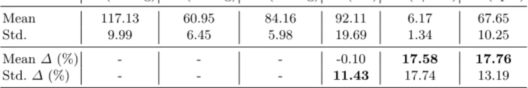
Overall (see Table 1), an increase of both the Heart Rate (HR) and the Cardiac Output (CO) of around 17% was observed. There were no significative changes in the values of the Systolic, Diastolic and Mean cuff pressure (SP, DP, MP) during the 1h process of digestion (beyond the intra-patient variability of the measurements). Finally the Stroke Volume (SV) was constant on average but the measurement showed a high inter-patient variability of the evolution (11%). Additionally, we tracked the boundaries of the endocardium over the entire cine MRI sequence acquired at T1, then extracted from this sequence a point at
SP (mmHg) DP (mmHg) MP (mmHg) SV (mL) CO (L/min) HR (bpm)
Mean 117.13 60.95 84.16 92.11 6.17 67.65
Std. 9.99 6.45 5.98 19.69 1.34 10.25
Mean ∆ (%) - - - -0.10 17.58 17.76
Std. ∆ (%) - - - 11.43 17.74 13.19
Table 1: Statistics of the measurements and their evolution ∆ between T1 and T2 (in percentage of the value at T1). Systolic, Diastolic and Mean cuff Pressure (SP, DP, MP), Stroke Volume (SV), Cardiac Output (CO) and Heart Rate (HR).
the apex of the left ventricle and one at the top of the left ventricle septum. This was used to calculate the Septal Shortening (SS) as the maximal shortening of the distance between these two points during the cycle. It has an average value of −17% and a standard deviation of 3.7% across the population.
3
Patient-Specific Cardiac Modelling
3.1 3D Electromechanical Cardiac Model
We performed 3D cardiac modelling for 21 of these patients. A high-resolution biventricular tetrahedral mesh of the patient’s heart morphology was extracted as in [6] from the pre-ingestion MRI at T1, made of around 15 000 nodes. On this
mesh, a myocardial fibre direction can be defined at each node of the mesh (see Fig 1a), by varying the elevation angles of the fibre across the myocardial wall from α1 on the epicardium to α2 degrees on the endocardium. In this paper,
α2 is set at the default value of 90o and α1 is a variable parameters in our
experiments.
Fig 1a: 3D heart geometry with my-ocardial fiber direction
Fig 1b: Schema and rheological model and of the windkessel model (figure from [7])
The depolarization times across the myocardium were computed with the Multi-front Eikonal method [8]. The APD is set from the Heart Rate with clas-sical values of the restitution curve and default values of conductivities are used as in [9]. Myocardial forces are computed based on the Bestel-Clement-Sorine model as detailed in [10]. It models the forces as the combination of an active con-traction force in the direction of the fibre, in parallel with a passive anisotropic hyperelasticity driven by the Mooney-Rivlin strain energy. In this paper, we only consider two main parameters of the model: the Maximal Contractility σ and the Passive Stiffness c1. Finally for the haemodynamics, the pressure in the
car-diac chambers are described by global values, and the mechanical equations are coupled with a circulation model implementing the 4 phases of the cardiac cycle [11].
In particular the pressure of the aortic artery Par(cardiac after-load) is
mod-eled with a 4-parameter Windkessel model [7], which describes the evolution of arterial blood pressure with the second-order equation of an electric circuit (see Fig 1b). The blood inertia is modeled by the inductance L, the arterial com-pliance by a capacity C and the proximal and distal (peripheral) resistances respectively by a resistance ZCand R (see Fig 1b). Finally, the venous pressure
Pvemodels the mean pressure in the venous system. In the following, ZCand L
are fixed at a default value (see [11]) while C, R and Pveare variable parameters.
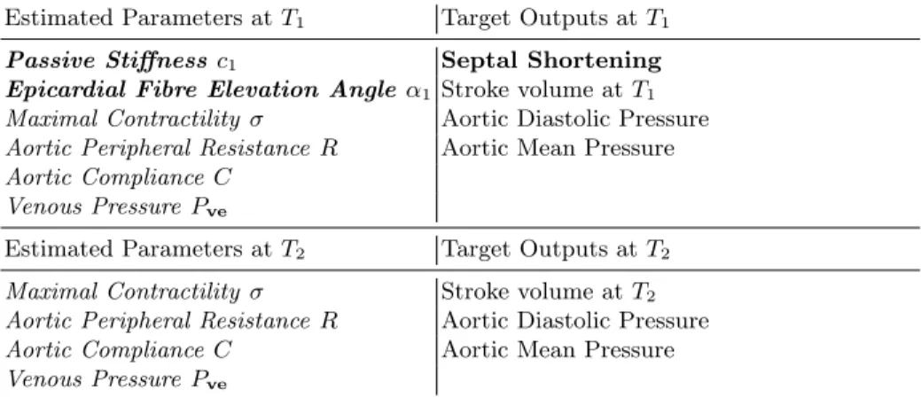
3.2 Longitudinal Parameter Estimation
After building the heart mesh geometry, parameter estimation is the next step in order to have model simulations which reproduce the available data. Considering a set of simulated quantities called the ”outputs” O (such as the Stroke Volume or the Mean Pressure for example), and a set of model parameters P , it consists in finding adequate values x of the parameters such that the output values O(x) in the 3D model simulation fit the ”target values” bO available in the data. This is done by performing an optimization of the parameter values x in order to minimize a distance S(x, bO) = ||O(x) − bO||S between the simulated values O(x)
and the target values bO (normalised to compare quantities with different units). For each patient, we have here measurements of different varying quantities at the two instants T1 and T2 (such as the stroke volume and the heart rate),
so we need to estimate different values for some cardiac model parameters (in particular the haemodynamic parameters) at these two instants. On the other hand, during the time-scale of the study (1h on average), some parameters of the cardiac model can be considered constant. This is the case of the Epicardial Fibre Elevation Angle α1 for example, or the cardiac stiffness c1. In order to
have consistent sets of estimated parameters at these two different instants, we need to use the same values for these parameters at these two instants.
To that end, we perform a two-step parameter estimation. First, we estimate values of both the fixed and varying parameters from the data at T1. Then we
reuse the estimated values of the fixed parameters for T2and estimate new values
we then have two distinct Parameter Estimation problems: the estimation of 6 parameters values in order to fit 4 target output values at T1(with the heart rate
of the simulations set to its value at T1). Then the estimation of 4 parameters
values in order to fit 3 target output values at T2(with the heart rate at T2).
Estimated Parameters at T1 Target Outputs at T1
Passive Stiffness c1 Septal Shortening
Epicardial Fibre Elevation Angle α1 Stroke volume at T1
Maximal Contractility σ Aortic Diastolic Pressure
Aortic Peripheral Resistance R Aortic Mean Pressure Aortic Compliance C
Venous Pressure Pve
Estimated Parameters at T2 Target Outputs at T2
Maximal Contractility σ Stroke volume at T2
Aortic Peripheral Resistance R Aortic Diastolic Pressure
Aortic Compliance C Aortic Mean Pressure
Venous Pressure Pve
Table 2: Estimated Parameters and Target Outputs in the parameter estimations at T1 and T2. Constant parameters whose values are reused for the estimation at T2 are outlined in bold. The heart rate in the simulations for the estimation at T1 (resp T2) correspond to the measured value at T1 (resp T2).
The optimisation was performed with an extended version of the framework described in [12]: the main algorithm is the CMA-ES genetic algorithm, which asks at each iteration for the score of a high number of 3D simulations. Instead of actually computing all these 3D simulations, we only compute a few within the parameter space (2N + 1 where N is the number of estimated parameters). Then we build a ”low-fidelity” surrogate model [13] from these simulations which allows to approximate the outputs of the 3D simulations for many successive iterations of the algorithm, without performing all the 3D simulations. This robust and efficient ”multifidelity optimization” allows a very fast exploration of large parameter sets with a low computational cost. In particular for the two problems at T1 and T2, we performed the optimization for the 21 patients
simultaneously and the convergence was reached in around two days.
4
Exploitation of Estimated Parameters
4.1 Analysis of Parameter Trends in the Population
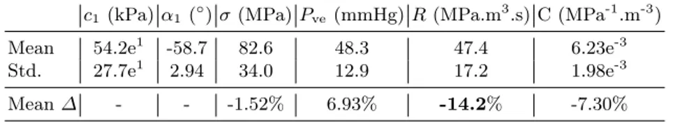
Across the 21 patients and the two estimations, the average fit error on the target ouput values are 1.9 mL for the Stroke Volume, 1% for the Septal Shortening, and 0.1 mmHg for both the mean and diastolic pressures, with few outliers. As
a consequence of this step, we now have a population of 21 personalised patient hearts at two instants. For each parameter, we report in Table 3 the mean and standard deviation of its estimated values at T1across the 21 patients, as well as
the mean of its evolution ∆ between the instants T1and T2 (difference between
the values estimated at T2and T1).
c1(kPa) α1 (◦) σ (MPa) Pve (mmHg) R (MPa.m3.s) C (MPa-1.m-3)
Mean 54.2e1 -58.7 82.6 48.3 47.4 6.23e-3
Std. 27.7e1 2.94 34.0 12.9 17.2 1.98e-3
Mean ∆ - - -1.52% 6.93% -14.2% -7.30%
Table 3: Statistics of the estimated parameters and of the difference ∆ between esti-mated parameters at T1 and T2
The first remark is that on average, the parameters R which models the arterial peripheral resistance decreases by 14%. This was expected and corre-sponds to findings in [3]. In a clinical setting the peripheral resistance is indeed computed as the ratio between the blood flow and the blood pressure, and a similar relationship can be derived in the model: as shown in Fig 2a the ratio (MP-Pve)/CO is almost exactly equal to the peripheral resistance R in our
simu-lations. Across the population, since the cardiac output CO increases by around 17% but the pressures are constant, the peripheral resistance has to decrease by a close number (14.2% here) on average.
We then notice both an average increase of the venous pressure Pve and
decrease of the arterial compliance C. These two trends can be explained as to compensate the decrease of the resistance and avoid a drop in the mean blood pressure. Indeed, in the model, a decrease of R leads to a decrease of the ”characteristic time” τ = RC at which the blood pressure decreases from the systolic pressure to the ”asymptotic pressure” Pve. A decrease of R only
leads then to a decrease of the mean pressure. On the other hand, a decrease of C leads to an increase of the ”pulse pressure” (difference between systolic and diastolic pressure) since C links an increase of arterial volume to an increase of arterial pressure with the formula C∆P = ∆V (a less compliant aorta has a higher pulse pressure for the same stroke volume). This contributes to the increase of the mean pressure (see Fig 2b), and it is also the case of the increase of Pve. Interestingly, we can note that these two trends (decrease of the arterial
compliance and increase of venous pressure) in parameters correspond to actual cardiovascular phenomena which are commonly observed during exercise [4, 5].
Finally, we can also observe a high correlation between changes in the Maxi-mal Contractility σ and changes in the ejected volume, as shown in Fig 2c. This is also a known phenomenon in cardiac dynamics, in particular at the core of the Starling Effect.
Fig 2a: (MP-Pve)/CO as a function of R Fig 2b: SV/(MP-DP) as a function of C Fig 2c: ∆σ (%) as a function of ∆SV (%)
4.2 Parameter Evolution Law
From this data and the estimated parameters, we then build a law f which, from a given simulation, gives variations of the electromechanical parameters σ, Pve, R and C which leads to a new simulation with prescribed changes in heart
period (HP) and stroke volume (SV) while having same mean and diastolic pressures: f (∆HP, ∆SV ) = (∆σ, ∆Pve, ∆R, ∆C)
This is done by computing a multivariate regression between the changes (in %) in Heart Rate and Stroke Volume and the changes in the estimated parameters values at the two instants T1and T2, for the 21 patients. We report
in Table 4 the coefficients of this multivariate regression:
Table 4: Coefficient of the multivariate regression f ∆ σ ∆ Pve ∆ R ∆ C
∆ HP -0.02 -0.15 1.20 0.51 ∆ SV 3.05 0.52 -1.04 1.19
The predicted variations of parameters with the variations of the heart period (∆HP) are consistent with the mean variations across the population described earlier. Interestingly with the coefficients of the second row (∆SV), we can also note how the parameters have to change for an increase in Stroke Volume only with constant pressures.
We finally tested the accuracy of this law with a leave-one-out approach: for each patient, we computed the regression f from the data and estimated param-eters of all the others patients. Then we changed the baseline paramparam-eters (at T1)
of this patient with the parameters predicted from f , and simulated the Pressure and Stroke Volume values at T2. The obtained results were accurate: on average,
the target Stroke Volume at T2 was predicted within 1.9 mL and the mean
ab-solute variations in Diastolic and Mean Pressure were within 2.1mmHG, which is beyond the variability of both the intra-patient and population variabilities.
5
Conclusion and Discussion
In this manuscript we performed a consistent longitudinal estimation of cardiac model parameters for 21 patient-specific hearts at two different instants within a 1h time span, from clinical data. This was done through two successive parameter estimation problems: we first estimated 6 parameters to fit the simulated Stroke Volume, the Septal Shortening and the Mean and Diastolic Pressures to their values at the first instant. Then we reused the estimated values of the fixed parameters at this step and performed a second estimation of 4 parameters to fit values of Stroke Volume and Pressures at the second instant. This was done in parallel for the 21 hearts in around two days and a maximum of 150 simulations of the 3D model per patient.
From those personalised hearts, we identified relationships between the esti-mated parameters and the simulated pressure and volume outputs, and linked their evolution between these two instants to classical physiological phenomena. Then we extracted a law which computes changes of electromechanical parame-ters from changes of stroke volume and heart rate with constant pressure. This law allows in particular to easily simulate the changes observed between the two instants without having to perform the parameter estimation step at the second instant. This was evaluated in a leave-one-out test and showed that it can predict accurately changes in the model parameters.
A first direct continuation of this work would be to quantify (from further data) to what extent this law holds for changes of cardiac outputs which are more important (digestion can be seen as a ’mild’ exercise and it is known for example that blood pressure rises during more intense exercises). Finally, for future patients, it could also be interesting to evaluate to what extent the changes in both the Stroke Volume and the Heart Rate can be predicted, and use our law to simulate the predicted heartbeats.
Ackowledgements This work has been partially funded by the EU FP7-funded project MD-Paedigree (Grant Agreement 600932) and contributes to the objec-tives of the ERC advanced grant MedYMA (2011-291080).
References
1. Laughlin, M.H.: Cardiovascular response to exercise. American Journal Physiology 277(6 Pt 2) (1999) S244–S259
2. Chabiniok, R., et al.: Multiphysics and multiscale modelling, data–model fusion and integration of organ physiology in the clinic: ventricular cardiac mechanics. Interface Focus 6(2) (2016)
3. Hauser, J.A., et al.: Comprehensive assessment of the global and regional vascular responses to food ingestion in humans using novel rapid mri. American Journal of Physiology-Regulatory, Integrative and Comparative Physiology 310(6) (2016) R541–R545
4. Otsuki, T., et al.: Contribution of systemic arterial compliance and systemic vas-cular resistance to effective arterial elastance changes during exercise in humans. Acta physiologica 188(1) (2006) 15–20
5. Albert, R.E., et al.: The response of the peripheral venous pressure to exercise in congestive heart failure. American heart journal 43(3) (1952) 395–400
6. Mollero, R., et al.: Propagation of myocardial fibre architecture uncertainty on electromechanical model parameter estimation: A case study. In: FIMH 2015, Springer 448–456
7. Westerhof, N., et al.: The arterial windkessel. Medical & biological engineering & computing 47(2) (2009) 131–141
8. Sermesant, M., et al.: An anisotropic multi-front fast marching method for real-time simulation of cardiac electrophysiology. In: FIMH 2007, Springer 160–169 9. Pernod, E., et al.: A multi-front eikonal model of cardiac electrophysiology for
interactive simulation of radio-frequency ablation. Computers & Graphics 35(2) (2011) 431–440
10. Chapelle, D., et al.: Energy-preserving muscle tissue model: formulation and com-patible discretizations. International Journal for Multiscale Computational Engi-neering, 10(2) (2012)
11. Marchesseau, S.: Simulation of patient-specific cardiac models for therapy plan-ning. Thesis, Ecole Nationale Sup´erieure des Mines de Paris (2013)
12. Mollero, R., et al.: A multiscale cardiac model for fast personalisation and ex-ploitation. In: MICCAI 2016, Springer 174–182
13. Peherstorfer, B., et al.: Survey of multifidelity methods in uncertainty propagation, inference, and optimization. (2016)