Analyzing Coherent Structures in
Two-Dimensional Dynamical Systems
by
Michael R. Allshouse
B.S. Mechanical Engineering (2008)
Massachusetts Institute of Technology
M.S. Mechanical Engineering (2010)
Massachusetts Institute of Technology
MASSACHUSESINSTYE
OF TECHNOLOGY
NOV 1 2 2013
LIBRARIES
Submitted to the Department of Mechanical Engineering
in partial fulfillment of the requirements for the degree of
Doctor of Philosophy in Mechanical Engineering
at the
MASSACHUSETTS INSTITUTE OF TECHNOLOGY
September 2013
©
Massachusetts Institute of Technology 2013. All rights reserved.
Author ..
....
7:
2
. . .
. . . . .
...
Spartment of Mechanical Engineering
August 16, 2013
Certified by...
Thomas Peacock
Associate Professor
) ,)esiSpervisor
Accepted by.
...-.
w.
. . . . . .. . . .David Hardt
Chairman, Department Committee on Graduate Studies
....
Detecting and Analyzing Coherent Structures in
Two-Dimensional Dynamical Systems
by
Michael R. Allshouse
Submitted to the Department of Mechanical Engineering on August 16, 2013, in partial fulfillment of the
requirements for the degree of
Doctor of Philosophy in Mechanical Engineering
Abstract
The identification of coherent structures enhances the understanding of transport
by complex flows such as those found at the ocean surface. The rapidly developing
approach of Lagrangian Coherent Structures (LCSs) is based on the identification of codimension-1 structures that are locally the strongest repelling material surfaces in forwards or backwards-time over a given time window. Current theory and methods regarding LCSs are surveyed, and we present a modified algorithm for their detection, highlighting the pros and cons of the modified approach. One beneficial aspect of the modified approach is that it is possible to classify and advect LCSs through the time window.
We apply the improved detection scheme as well as the classification to a high quality, validated simulation of ocean surface flow near the Ningaloo reef along the coast of Western Australia. This region is home to the longest fringing reef in Aus-tralia, a diverse marine environment, and a growing offshore drilling industry, and understanding the surface flows will enable better informed decisions to be made in this environmentally delicate domain. In addition to applying the LCS techniques, for the first time we account for the impact of surface winds on the LCS field by creating a hybrid current-wind velocity field.
While the LCS approach is based on rigorous dynamical systems theory, its re-liance on an accurate velocity field restricts potential ocean applications to simulations or regions with surface velocity measurements via systems like HF radar stations. An untapped resource is the data collected from float trajectories. With the goal of eventual application to these data sets, we develop a coherent structure detection algorithm utilizing sparse trajectory data. This new approach is based on the ap-plication of tools from braid theory, which produce a simplified perspective of the mixing of two-dimensional systems that enables rapid analysis. As a first application, our braid-based approach is applied to a periodically stirred system.
Thesis Supervisor: Thomas Peacock Title: Associate Professor
Acknowledgments
Through nine years at the institute, there have been countless people who have af-fected my experiences, and unfortunately I do not have the space to thank them all.
I highlight those of particular impact on my Ph.D. studies, but am eternally grateful
to the entire MIT community for making my time here enjoyable and enlightening. First and foremost, I must thank my advisor of six years Professor Tom Peacock, despite his allegiance to the white half of London. I could not ask for a more sup-portive and engaging advisor. He has afforded me countless opportunity to travel and interact with the greater coherent structure community. It is his endless optimism that has guided me through this thesis, and for all of this I thank him.
Next, I also thank my advisor from the GFD summer school, Professor Jean-Luc Thiffeault of the University of Wisconsin. He introduced me to the world of topology and braids, and was remarkably patient as I fumbled through the details. He gra-ciously hosted me for a semester in Madison, allowing me to experience the academic world outside of MIT. Professor Thiffeault was a constant source of entertaining tan-gential information, and it was a pleasure working with him.
I would also like to recognize the other members of my thesis committee, Professors Lermusiaux, Pratt, and Turitsyn. Each of you were of great help in framing my work and providing unique insights. Thank you all for your help throughout the committee meetings, thesis writing, and defending processes.
A number of people from the coherent structure community also aided this work
through conversation and collaboration. Mohammad Farazmand, George Haller, Josefina Olascoaga, and Wenbo Tang all provided insight in the development of a number of the LCS codes. Despite not being presented in this thesis, CJ Beegle-Krause assisted in data acquisition and interpretation for the Gulfs of Alaska and Mexico. Nick Ouellette and Doug Kelley collaborated with me on an application of LCS. Shawn Shadden, Mark Stremler, and Phil Boyland all provided intriguing
conversation.
conver-sation, tolerance, and friendship. In particular, Mani Mathur and Sasan Saidi spent many years with me and were supportive through the peaks and valleys of research. Matthieu Leclair, though briefly overlapping, was able to turn my codes into efficient tools for wider use.
Support from administrative members of the lab and department enabled me to focus primarily on research while they managed the logistics. Ray Hardin was a constant joy to interact with and artfully juggled all of his responsibilities to provide a stable work environment. Leslie Regan and Joan Leonard provided support in taking care of departmental and institute matters.
My friends and family have provided support and distraction when I needed it
most. In particular, my parents were always willing to listen to me talk in gibberish but always assured me that I would figure out a way. John, Stephen, Chun, Justin, Cokie, Ali, Steven, Helen, and Jo, each of you provided the best distractions from work to keep me sane.
Nina, you made all nine years at MIT a joy. You pushed me to expect the most out of myself, and knew when to step aside so that I could work towards that. We are always better together.
To the One who was with me from the beginning, for the strength when I had none left.
Contents
1 Introduction
1.1 Coherent structures . . . .
1.1.1 Eulerian structures . . . .
1.1.2 Mesohyperbolic and mesoelipitic structures
1.1.3 Ergodicity and complexity measures...
1.1.4 Perron-Frobenious operator approach . . . .
1.1.5 Invariant (KAM) tori . . . .
1.1.6 Lobe dynamics . . . .
1.2 Lagrangian Coherent Structures . . . .
1.3 Applications of LCS . . . .
1.3.1 Application to laboratory experiments . . .
1.3.2 Application to geophysical datasets . . . . .
1.4 Thesis outline . . . .
2 Investigations of established LCS practices
2.1 Background and motivation . . . . 2.2 Analytic Models . . . . 2.2.1 Autonomous System . . . . 2.2.2 Non-Autonomous System: Double-Gyre . . 2.3 Flow M ap . . . . 2.4 Flow Map Gradient . . . . 2.4.1 Finite Difference (FD) Cluster Method . . .
2.4.2 Advected Gradient (AG) Method . . . .
11 . . . . 12 . . . . 13 . . . . 14 . . . . 16 . . . . 17 . . . . 18 . . . . 19 . . . . 21 . . . . 23 . . . . 23 . . . . 25 27 29 . . . 29 . . . 33 . . . 34 . . . 36 . . . 37 . . . 40 . . . 41 . . . 42
2.5 Right Cauchy Green (CG) deformation tensor
2.6 Comparison between FD and AG
2.6.1 Autonomous system study
2.6.2 Double-gyre study . . . .
2.6.3 AG vs. FD conclusions . .
2.7 Strainlines and Shearlines . . . .
2.7.1 Normal Vector Advection
2.7.2 Strainlines . . . .
2.7.3 Shearlines . . . .
2.7.4 A shear example... 2.8 Variational LCS and geodesic LCS
2.8.1 Variational LCS . . . . 2.8.2 Hyperbolic Cores... 2.8.3 Geodesic LCS . . . . 2.9 Method Conclusions . . . . nethods . . . . and hyperbolic
3 Identification and classification of LCS as FTLE
3.1 FTLE Ridges . . . . 3.1.1 Ridge Definition . . . . 3.1.2 Ridge Tracking . . . . 3.1.3 Ridge Refinement . . . . 3.1.4 Ridge Application . . . . 3.2 Ridge Classification . . . .
3.2.1 Previous Classification Schemes . . . .
3.2.2 Classifications . . . .
3.2.3 Normal versus Tangential Growth . . . . .
3.2.4 Normal Repulsion versus Lagrangian Shear
3.3 Methods application and discussion . . . .
3.3.1 Application to analytic systems . . . .
3.3.2 Application to discretized Double-Gyre system .
cores 45 46 48 50 52 53 55 58 60 62 62 64 66 68 ridges 71 . . . . 71 . . . . 72 . . . . 75 78 . . . . 80 . . . . 85 85 . . . . 88 . . . . 88 92 . . . . 95 . . . . 96 108 . . . . 44
3.4 FTLE Ridge Conclusions ...
4 Application of LCS methods to Ningaloo Region
4.1 The Ningaloo peninsula ...
4.2 Numerical model ... 4.3 LCS analysis ... 4.4 LCS Results ... 4.4.1 Time window 1 ... 4.4.2 Time window 2 ... 4.5 Windage Study ... 4.5.1 Implementation ... 4.5.2 Results ...
4.6 Discussions and Conclusions ...
5 A braid theoretical approach
5.1 Introduction to braid based coherent structures . ...
5.2 Braid theory and topological surface dynamics . . . . .
5.2.1 Physical braids . . . .
5.2.2 Generators . . . .
5.2.3 Loops . . . .
5.2.4 The action of generators on loops . . . .
5.2.5 How the topological tools fit together . . . .
5.3 Search for non-growing loops: Direct method . . . .
5.3.1 Simple loops . . . .
5.3.2 Algorithm outline . . . .
5.3.3 Modified Duffing oscillator . . . .
5.3.4 Results of the direct method . . . . 5.4 Search for non-growing loops: Pair-loop method . . . .
5.4.1 Step 1: Application of generators to pair-loops . 5.4.2 Step 2: Determine the entangled puncture sets . 5.4.3 Step 3: Find the invariant puncture sets . . . .
112 115 . . . . . 116 . . . . . 118 . . . . . 120 . . . . 123 . . . . 124 . . . . 136 . . . . 144 . . . . 144 . . . . 146 . . . . 151 155 . . . . 156 . . . . 158 158 . . . . 159 . . . . 160 . . . . 163 . . . . 164 . . . . 165 . . . . 165 166 . . . . 166 167 . . . . 170 . . . . 171 . . . . 173 174
5.4.4 Step 4: Creation of slow-growing loops . . . . 176
5.4.5 Application to the modified Duffing system . . . . 178
5.5 Finding non-growing loops in a rod-stirring device . . . . 179
5.6 Conclusions . . . . 181
6 Conclusions 183 6.1 Summary of results . . . . 183
6.2 Future works . . . . 185
A Autonomous System Derivation 187 B Preservation of orthogonality after mapping 191 C Derivation of p and - 193 D Derivation of strainline and shearline tangent fields 197 D .1 Strainlines . . . 197
D.2 Shearlines . . . . 199
E Analysis of error in eg, ng, p, and o 203
Chapter 1
Introduction
On 20 April 2010, an explosion 40 miles off the coast of Louisiana resulted in eleven deaths and the sinking of the Deepwater Horizon oil rig. For the next 87 days, the blown out wellhead proceeded to pump 4.9 million barrels of oil into the Gulf of Mexico making it the largest accidental oil spill in history. Less than a year later on 11 March 2011, a magnitude 9.0 earthquake 43 miles to the east of Japan resulted in a massive tsunami causing wide spread destruction. Large amounts of debris, some being radioactive, was drawn out into the ocean and drifted as far as the American West Coast. In the wake of these disasters, efforts were made to predict and understand the transport of the oil and debris, respectively, in order to formulate response plans to contain the contaminants. A useful tool for this analysis is coherent structure detection, which has the ability to analyze large amounts of simulated or measured velocity data and produce a simplified description of the system's transport dynamics.
We begin this chapter, and thesis, by presenting a variety of alternative coherent structure definitions and approaches in section 1.1. Ultimately, we have selected the definitions and methods of Lagrangian Coherent Structures (LCSs) as one of the primary focuses of the research, and a brief introduction to the topic is presented
in section 1.2. Particularly relevant or revolutionary applications of LCS theory are discussed in section 1.3, revealing the state of the art of application and providing some insight into possible improvements of the theory. Finally, we present an overview
(a) (b)
Figure 1-1: (a) Satellite image of Deepwater Horizon oil spill on 17 May 2010 (Image adapted from http://www.space.com/) (b) Tdhoku Tsunami debris island stretching 60 miles and covering 2.2 million square feet (Image reproduced from http://www.telegraph.co.uk).
of the thesis, in section 1.4, which will discuss the development of new LCS tools, their application to an ocean simulation, and the creation and application of a new type of coherent structure approach based on the topic of braid theory.
1.1
Coherent structures
Coherent structures are reduced order features in a fluid flow (e.g. one-dimensional material lines in a two-dimensional flow) that provide a decomposition of the system into dynamically distinct domains. This definition is intentionally left broad because it encompasses a wide variety of approaches for identifying such features. These structures have the ability to capture events such as filament formation or large scale bulk transport, as seen in figures 1-1(a) and (b), respectively. Here we summarize a number of alternative, established approaches to identifying coherent structures in fluid flows before introducing the theory of Lagrangian Coherent Structure (LCS), which is a focus of this thesis. The scope of this survey is limited to approaches that have been generalized and applied to aperiodic, finite-time flows.
1.1.1
Eulerian structures
The Eulerian specification of dynamical systems observes properties such as velocity, acceleration, or vorticity at particular locations regardless of which fluid element is present at any instant in time. Eulerian coherent structures attempt to partition the flow at a given time based on frame dependent scalar fields such as vorticity, kinetic energy, or strain. Some examples of Eulerian coherent structures identify regions with phase-correlated vorticity (Hussain, 1986), regions bound by vorticity gradients (Juckes & McIntyre, 1987), or regions with high vorticity (Benzi et al., 1988),
One approach that seeks to differentiate hyperbolic and elliptic (e.g. vortex) structures is the Okubo-Weiss criteria (Weiss, 1991). The metric:
Q(x, t)
=
s
2(X, t) - w
2(x, t),
(1.1)
measures the difference between the squared vorticity,
2 = U2 Ou1 2
(X
1 1X2and squared strain:
2
Bu
10u
2 2 8U2 + u1 2s
=
+
)
+
2
)-
Kaxi
ax
2dxi
8x
2given the velocity field u = (ui, u2) and the coordinates x = (XI, x2). Hyperbolic regions and elliptic regions are designated by subdomains where Q(x, t) > 0 and
Q(x, t) < 0, respectively. The range of validity of the Okubo-Weiss criteria was
tested by Basdevant & Philipovitch (1994), who demonstrate that only very close to the center of hyperbolic and elliptic regions is the criteria valid.
There are two main drawbacks to Eulerian based coherent structure detection. Because the structures are based on Eulerian data, they are identified at each time instance independently. When viewing the time evolution of structures, there is no inherent relationship between the time dependent system decomposition and the par-ticular fluid elements separated by a given structure. This does not lend itself to
f
sin4t 2+cos4r x 10 i0'v(x,ye) = II(f I II
-2+cos4t -sin4 y 0p
-a-> Switch to rotating frame:
---x cos2t sin2tf i y -sin2t cos2t
Figure 1-2: An example system where the qualitative flow and the Okubu-Weiss criteria changes from elliptic to hyperbolic when viewed from a rotating frame.
analyzlig the transport of particular fluid over a time window, which is an objective of this thesis. The second concern is that these structures are not frame invariant. Because the Eulerian coherent structures rety on frame dependent quantities, chang-ing the frame of reference can fundamentally change the decomposition of a system.
An example of this is presented in figure 1-2, where an elliptic type flow ilk a
station-ary frame becomes a hyperbolic flow when viewed from a rotating frame of reference. This qualitative change is manifested by the change in Okubu-Weiss value from being negative to positive. Since the shape of material structures is not dependent on the frame of reference from whiich they are observed, it is imperative that this should also be the case for the coherent structures identified in fluid flows.
1.1.2
Mesohyperbolic and mesoelipitic structures
Differentiation between elliptic and hyperbolic type flow features was extended by Mezi6 et al. (2010). As opposed to analyzing the instantaneous velocity field, the au-thors calculate the so-called average Lagrangian velocity. u*. from which they identify regions that on average demonstrate elliptic or hyperbolic behavior. This field requires the calculation of trajectories by solving the ODE:
.. . .-
.-(a) (b)
Figure 1-3: Lagrangian flow field around points where (a) detVu* < 0 and (b) detVu* > 4/T 2. Select trajectories (green), strongest repelling line (red), and strongest attracting line (blue) are presented to highlight the flow features.
with initial condition xo at time to for the time window t = [to to + T]. The average Lagrangian velocity is defined as:
u* (xO) =
x(toT)-xo
(1.3)T
which corresponds to the displacement of a given point divided by the length of the time window. At each point the Jacobian of the average Lagrangian velocity field is calculated, Vu*, and its determinant is the metric used by the criteria.
The criteria proposed by Mezi6 et al. (2010) decipher between mesohyperbolic and mesoelliptic regions, which are sets of Lagranian points that experience local hyperbolic or elliptic type deformation during advection. A Lagrangian point labeled as mesohyperbolic satisfies the condition detVu* < 0 or detVu* > 4/T2, which correspond to local average Lagrangian flow fields of the types presented in figures 1-3(a) and (b), respectively. Mesoelliptic regions contain points where 0 <detVu* < 4/T 2 representing rotation dominated local flows. While there is no time-dependence in classification, this approach still relies on the frame dependent measure of the gradient of the average Lagrangian velocity, and thus is not frame invariant.
1.1.3
Ergodicity and complexity measures
While Mezi6 et al. (2010) was concerned only with final trajectory displacement, the complexity measures developed by Scott et al. (2009) and Rypina et al. (2010) consider the entire trajectory history. The core assumption made by both complexity measures is that smooth barriers divide the system into chaotic mixing regimes, and the barriers themselves remain smooth throughout advection. Based on this premise, both measures identify coherent structures as one-dimensional low complexity curves dividing regions of high complexity.
Scott et al. (2009) defines the ergodicity defect, d, which compares particle res-idence time versus the fraction of the domain visited. In regions of chaotic flow, a trajectory spends little time in any particular location and visits a large fraction of the domain; this results in an ergodicity defect of d = 0. Conversely, stationary
points remain in the same space for the entire time window resulting in d = 1. Based
on these extremes, coherent structures are defined as lines of locally maximum er-godicity defect. Another complexity measure proposed is the correlation dimension, c (Rypina et al., 2010). Ranging from c = 0 (stationary point) to c = 1 (smooth
one-dimensional curve) to c = 2 (chaotic curve densely covering a two-dimensional area), this measure analyzes how densely a trajectory explores the domain. In this case, the coherent structures are troughs of the correlation dimension field.
These measures, as well as other trajectory based measurements, provide a frame invariant classification of trajectories, but thus far application has been limited. One significant benefit of this type of measure is its reliance on only isolated trajectory information making application to ocean drifter datasets possible. However, the accu-racy of the structure identification is limited by the density of initial conditions, and a high density of trajectories is uncommon in drifter datasets. Additionally, while there is good agreement between these results and the ones drawn from the LCS theory that is a focus of this thesis (Rypina et al., 2011), the theoretical development of these measures is still in progress.
1.1.4
Perron-Frobenious operator approach
Similar to the Mezi6 et al. (2010) method, the Perron-Frobenious transfer operator approach relies on the initial and final position of trajectories. This approach identifies pairs of closed boundaries at the beginning and end of the time window that initially surrounded portions of the domain that escape the corresponding final time boundary with low probability (Dellnitz & Junge, 1999). A sketch of boundaries with a high (black) and low (red) probability of escape is presented in figure 1-4. These boundaries are identified by analyzing the transfer operator, P, which measures the probability that a point initially in the subdomain A advects to subdomain B. In practice, the transfer operator requires the domain be divided into small boxes, and then calculates the probability that a particle started in box i advects to box j, Pj. This leads to
the estimate for the probability that a particle in A advectes to B:
Y((x E A) E B) = E
PiS
iEA,jEBwhere 0 is the mapping function that determines where the point x advects to. The algorithm presented in Froyland et al. (2010) performs an optimization to identify the pair of equally sized boundaries that maximize the probability of advecting particles from the initial to the final boundary.
The probabilistic approach does a good job of identifying subdomains of the sys-tem that remain as compact sets moving through the domain during advection. Un-fortunately, these sets are often leaky, meaning that they do not retain all of the initial fluid during advection as the red domain demonstrates in figure 1-4. Also, in order to calculate the probabilities for the transfer operator accurately, a very large number of trajectories must be calculated. For each box subdividing the domain, hun-dreds of uniformly distributed particles are advected, which as the box size resolution decreases can result in millions of trajectories being calculated.
(a) (b)
Figure 1-4: (a) Distribution of initial trajectory position (blue and green), initial boundaries (red and black), and underlying boxes. (b) Final position of trajectories and boundaries. The red domain has low probability of escape and black has higher probability of escape.
1.1.5
Invariant (KAM) tori
Similar to the probabilistic approach, invariant (KAM) tori identify closed coherent structures that divide a region of fluid from the rest of the domain (Arnol'd et al.,
2006). Given a steady flow, if closed, periodic trajectories exist, the set of points
making up each trajectory, by uniqueness, form a boundary around some subdomain preventing transport of fluid into or out of the subdomain. Under small periodic per-turbations the previously periodic trajectories lose their periodicity, but in some cases new nearby periodic trajectories form, creating a new closed subdomain (Kolmogorov, 1954). The breakdown of invariant tori when noise is added is a result of resonance matching between the noise and the periodicity of tori, which limits the applicability to small, multiply-periodic (finite number of frequencies) perturbations. Methods for calculation have been developed and applied to geophysical meandering jets (Beron-Vera et al., 2010) and to identifying robust transport barriers in atmospheric zonal jets around the Antarctic ozone hole (Rypina et al., 2007). It was determined that these invariant tori are linked to the LCS approach we study (Haller & Beron-Vera,
2012).
**1?*,
/// t \t \ 0.5, 0.5-C 0 MW0 C 1 -0.5 - 0.5-I N ±LiZ _L IWL -1 -0.5 0 0.5 1 -1 -0.5 0 0.5 1 -1 -0.5 0 0.5 1 x1 :1 a:1 (a) (b) (c)
Figure 1-5: Velocity field around a hypberoblic point (black arrows), the unstable (blue) and stable (red) invariant manifolds, stemming from the hyperbolic point (the origin). Passive tracer patches (shades of green) at times (a) t = -1.5, (b) t = 0, and
(c) t = 1.5.
1.1.6
Lobe dynamics
While both invariant tori and almost invariant sets identify closed regions surrounded
by a single coherent structure, lobe dynamics studies the transport of fluid captured
between two different structures forming a closed barrier. The theory was developed for two-dimensional periodic (MacKay & Tresser, 1984; Ottino, 1989; Wiggins, 1991) and quasiperiodic systems (Beigie et al., 1991), and application of the theory was extended to finite-time aperiodic systems by (Miller et al., 1997).
Lobe dynamics applies the concepts of hyperbolic points and invariant manifolds; both of which are pertinent to LCS theory. An example of a hyperbolic point is presented in figure 1-5 and is characterized by the attraction of material in two direc-tions and repulsion of material in two other direcdirec-tions. In figure 1-5, material from the left and right moves towards the origin only to be repelled up or down. In this case, there is an autonomous (time-independent) flow, so the hyperbolic point (the origin) remains stationary. For time varying flows, a Lagrangian hyperbolic point moves through the domain and has a hyperbolic Lagrangian velocity field (velocity field relative to the point) similar to the one presented in figure 1-5 throughout the time window.
The other important features in figure 1-5 are the stable and unstable invariant 0. -0 A,//t \ \\\ 5- 0- .5-S '.~N\ I /,.Z
manifolds, which by uniqueness divide the system into dynamically distinct domains.
A hyperbolic point, p, has a corresponding stable invariant manifold, W8(p), defined
as the set of points that asymptotically approach the hyperbolic point, as t -+ oo.
Similarly, the unstable invariant manifold, WU(p), is defined as the set of points that asymptotically approach the hyperbolic point as t -+ -co. These manifolds are presented in figure 1-5 as red and blue lines, respectively. In forwards-time, the tracer patches are repelled away from the stable manifold and attracted to the unstable manifold, and the opposite is true in backwards-time (time run in reverse).
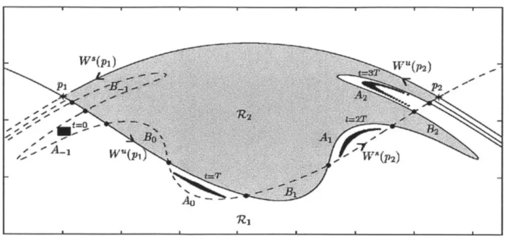
Lobe dynamics studies the mechanism of transport between regions separated by the invariant manifolds of two nearby hyperbolic points within a periodic flow. A schematic of the transport is presented in figure 1-6, and due to the periodicity of the flow the hyperbolic points return to their initial position at the conclusion of each period. As a result of their infinite length, the invariant manifolds appear to return to the same place when in fact all points on the manifold are advecting closer or further from the hyperbolic points with each period. The two hyperbolic points pi and P2 are connected by the trajectory consisting of W'(pi) and W'(p2). Meanwhile, the invariant manifolds W(pi) and W,(p 2) form enclosed regions like AO and BO in
figure 1-6. During the periodic advection, material within region AO moves to region A1 and particles in BO move to B1 after a period of advection as demonstrated by the
black, passive tracers in figure 1-6. After another period of advection the particles move to A2 and B2, and this process continues indefinitely. These lobes are important
because they take particles initially in R1 and transport them into R2 and vice versa.
While lobe dynamics and invariant manifolds do well in explaining the transport in these periodic infinite time systems, for applications to ocean flows, datasets never have infinite time lengths or perfect periodicity. Miller et al. (1997) took steps to ex-pand the theory to finite-time and aperiodic velocity fields. In place of the invariant manifolds, the finite time structures are found by advecting particles initially near the hyperbolic points. In the aperiodic flows, the hyperbolic points and invariant manifolds are free to move about the domain, so advection of these structures is
nec-P2.
Figure 1-6: Schematic of transport between R1 to 1Z2 via lobes formed by W"(pi)
and W'(p2
)-essary to understand the transport of the lobes in the domain. The advection reveals that lobes do not exist for the entirety of the time window Miller et al. (1997). While Miller et al. (2002) identified two nearby hyperbolic point in an ocean simulation and implemented the lobe approach to this aperiodic system, there is no guarantee of these types of systems existing in general flows. Finally lobe dynamics presents a graceful understanding of transport, but as the complexity of the system increases the lobe features become too numerous to account for making flux calculations unwieldy.
1.2
Lagrangian Coherent Structures
While Miller et al. (1997) created a heuristic approach to identifying the coherent structures forming lobes, Haller (2001) developed a more general approach to locate the LCS of a general dynamical system. Recognizing that invariant manifolds are the material lines most responsible for shaping transport, the theory aims to identify their analogs in finite time. Because the invariant manifolds can be characterized by their repulsion and attraction, the theory identifies a metric to measure the separa-tion between two neighboring particles for finite-time. From dynamical systems, the Lyapunov exponent measures the exponential rate of separation of two points initially infinitesimally close together (Lyapunov, 1992; Oseledec, 1968). For two points in a
- - --~:- --- -~-
chaotic system with initial distance apart, 6x, the separation is approximated as:
I Jx(t)|
~-.
e "IIJ
(0) 1,where A is the Lyapunov exponent. More formally, the maximal Lyapunov exponent is defined as:
1
16x(t)I
A = lim lim - log . (1.4)
IJX(tO)I-+O t-+oo t IJX(tO)I'
While Haller (2001) was not the first to create a finite-time analog (Wolf et al.,
1985; Pierrehumbert & Yang, 1993; Doerner et al., 1999), he was the first to utilize
the Cauchy Green deformation (CG) tensor, C, in order to define the finite time Lyapunov exponent (FTLE):
1
= -log A2 (1.5)
2t
where A2 is the largest eigenvalue of the CG tensor and t is the length of the finite-time
window. These concepts are further developed in chapter 2.
Haller (2001) identified local extrema of the FTLE field in forwards and backwards-time to locate LCSs. For a given backwards-time window T = [to t], the forwards-time FTLE field measures the repulsion of particles, and the local extrema of this field identify the location of repelling LCSs at time to. Calculating the FTLE field over the backwards-time window T = [t to] measures the amount of forwards time attraction, and the local extrema correspond to the position of attracting LCSs at time t. To compare the positions of repelling and attracting structures at some time, r in the window, it is necessary to advect the position of one or both types of structures to their posi-tion at r. This is often overlooked in many presentaposi-tions of FTLE results. Another, common mistake is to perform the forwards-time calculation over the time window T = [to to
+
t] and backwards-time calculation over the window T = [to to - t]. While this does identify the positions of attracting and repelling structures at time to, these results are not dynamically consistent because they do not span the same time window.formalized the definition of LCS as FTLE ridges calculated for a sequence of time intervals. Haller (2011) then modified the definitions of LCS to no longer be FTLE ridges but maximal lines of normal repulsion, strainlines. Most recently the theory has been expanded to include invariant tori like structures in Haller & Beron-Vera (2012). We do not discuss these advances in detail here as they are covered in depth in chapter 2.
1.3
Applications of LCS
A wide range of attempts have been made to apply LCSs to the study of experimental,
geophysical, atmospheric, and biological systems. The experimental applications of
LCS theory demonstrate that these structure do exist in real world environments and
have physical consequences. Because experimental measurements are noisy, these studies act as a filter to remove sensitive tools and develop robust replacements. The experimental results are followed by a sequence of studies of both observed and simulated atmospheric and oceanic systems. These studies reveal how locating LCSs can explain environmental events. Finally, in recent years there have been a number of exciting applications of LCS to biological systems. Because our primary interest is in application to ocean systems, we refer the reader to Peng & Dabiri (2009), Olascoaga (2010), and Hendabadi et al. (2013) for three unique applications of LCS theory to biological systems. While the following survey is not comprehensive it aims to highlight particularly novel applications and extensions of LCS theory.
1.3.1
Application to laboratory experiments
Voth et al. (2002) perform a sequence of two-dimensional, time-periodic experiments, which tracked particle motion as well as the distribution of fluorescein dye. From the data recorded over hundreds of forcing periods, a time-periodic velocity field is extracted and analyzed to calculate the backwards-time FTLE field and correspond-ing attractcorrespond-ing structures. Voth et al. (2002) then compare these structures to the spatial distribution of the dye concentration (see figure 1-7). They find that lines of
Figure 1-7: Distribution of dye (grey-scale) and attracting structures from an exper-imentally produced two-dimensional, time-periodic flow. Lighter regions correspond to lower concentration of dye and the attracting structures are calculated from the deformations over three periods. Figure reproduced from Voth et al. (2002).
constant dye concentration closely align with attracting structures under a variety of initial times and forcing frequencies. The study then identifies local hyperbolic and elliptic points in the periodic velocity field, and a direct relationship is found be-tween the position of the hyperbolic points and regions where attracting and repelling structures overlapped. While hyperbolic points always correspond to the crossing of structures, the reverse does not always hold and this inconsistency is not investigated. Additionally, it is ambiguous whether or not the attracting and repelling structures are calculated over the same time window, which might explain the inconsistencies between hyperbolic points and structure crossings.
While the experiments in Voth et al. (2002) are primarily laminar, a study by Mathur et al. (2007) analyzes a two-dimensional turbulent flow. The tall, rotating water column contains an approximately two-dimensional turbulent flow near the surface that is visualized to extract the velocity field. The data is used to create an FTLE field, from which Mathur et al. (2007) attempted to precisely find points of maximum FTLE value by advecting along the FTLE gradient. They also attempt to identify hyperbolic cores by locating positions where the rate of strain normal to the repelling structures is positive. Unfortunately, the authors do not use a dynamically consistent time window for their forwards and backwards-time calculations, so their
hyperbolic core test relies on hyperbolic activity at a single point in time as opposed to hyperbolic flow throughout a dynamically consistent time window.
The final experimental study we review attemptes to link the position of the LCS to the dynamical measure of average Lagrangian spectral energy flux (Kelley et al.,
2013). A quasi-two-dimensional, weakly turbulent flow, is measured and the resulting
FTLE field and corresponding repelling LCSs are calculated. Kelley et al. (2013) cre-ate the new dynamical measure: Lagrangian-averaged scale-to-scale spectral energy
flux, which filteres the velocity field and measures the scale-to-scale flux of energy
along a Lagrangian trajectory. This analysis tool indicates if energy is being trans-ported up or down the spectrum along particular trajectories. Combining this new diagnostic with the repelling LCS, the authors find statistically significant alignment between repelling LCSs and the division between regions with positive and negative flux. This study is the first to link LCS to any sort of energy transport indicating that LCS can be used to better understand the energy dynamics of turbulent flows.
1.3.2
Application to geophysical datasets
The first application of LCS theory to ocean measurements was by Lekien et al.
(2005) who analyze data from very high frequency (VHF) radar measurements of
surface flows off the coast of Florida. One issue encountered during FTLE calculations is particles escaping through open boundaries. The authors choose to simply stop advection once a trajectory reached a boundary, which results in a spatially varying integration time. Because of the inconsistency of integration time, spurious structures can form (Tang et al., 2010) such as those seen near (-80.1', 26.070) in figure 1-8. Despite these spurious features, Lekien et al. (2005) are able to demonstrate that particles released either side of a repelling LCS move to very different regions of the domain. They use the position of repelling structures to create a guidance system for when pollution should be released in the domain. A similar analysis of VHF radar in the Monterey Bay was performed by Coulliette et al. (2007). Lermusiaux et al.
(2006) also performed an FTLE analysis of Monterey Bay.
26,1 26.08 26.04 .26.04 -80.1 -80.075 -80.05 -80.025 Longitude (degrees)
Figure 1-8: Forwards-time FTLE field derived from VHF radar readings off the coast of Florida. Figure reproduced from Lekien et al. (2005).
simulation of Hurricane Isabel. While Lekien et al. (2005) view pollution as a passive tracer, Sapsis & Haller (2009) took the step to consider how inertial effects influence particle trajectories by adding an inertial term to the velocity equations. Performing one of the first non-analytic three-dimensional simulations, the authors were able to make rough approximations for the location of the hurricane's eye based on the attracting structure of aerosols.
Olascoaga & Haller (2012) present another study of how LCS theory can be used in understanding the advection of pollution. In this case, they focus on the previously discussed Deepwater Horizon spill of 2010 and locating influential hyperbolic cores. As opposed to Mathur et al. (2007), trajectories are required to be locally hyperbolic throughout the entire time window to be considered a potential core. While a number of potential cores may exist along a given LCS, the authors select to highlight struc-tures with the strongest normal repulsion at the end of the time window. The authors claim that these cores can be used for the prediction of major flow deformations in the near future. Over the period of 13 May to 17 May 2010 a long filament protrudes from the main oil spill site extending dangerously close to the Gulf of Mexico's Loop Current (see 1-1(a)). The authors identify a hyperbolic core, which accurately predict the filamentation days before it actually occurs. Their definition is discussed further in section 2.8.2
over the Hong Kong International Airport and attemptes to classify the LCSs. The two-dimensional velocity fields measured by radar span an open boundary, but unlike Lekien et al. (2005) the authors implement a finite domain technique, which removes spurious structures and covers a dynamically consistent time window (Tang et al., 2010). As mentioned in Shadden et al. (2005), regions of high shear can create high FTLE values just like hyperbolic points, so Tang et al. (2011) attempt to differentiate between such structures by implementing a classification method. We discuss this classification and potential problems in section 3.2.
1.4
Thesis outline
To date, all LCS studies seem to neglect presenting a detailed convergence analysis. Upon investigation and attempting reproduction of several key results, we found that under scrutiny many of the commonly used metrics break down primarily because they rely on gradient of numerical data. We begin with a thorough review of the fundamental concepts of current LCS theory in chapter 2, addressing the concepts of the flow map and its gradient. These concepts are then applied to a pair of analytic examples and convergence tests are discussed. While all studies so far have calculated the flow map gradient using finite difference, an alternative method is presented and the two are compared for the analytic system. Then the CG tensor and its eigenvalues and eigenvectors are discussed. Finally, we present a discussion of the variational LCS of Haller (2011), geodesic LCS of Haller & Beron-Vera (2012), and the hyperbolic cores of Olascoaga & Haller (2012).
The developments of Haller (2011) and Haller & Beron-Vera (2012) change the definition of LCS away from maximally repelling material lines. We return to the definition of LCS as the ridges of the FTLE field. In chapter 3, we present the defini-tion of a ridge that robustly captures these structures. An algorithm for identifying such ridges is presented along with a refinement scheme to improve the position ac-curacy. Because the structures repel nearby material, any error in the LCS position is magnified during advection. Our refinement scheme produces sufficient accuracy
to reliable advect the structures making direct comparison between attracting and repelling structures a reality. With the accurately located LCS, we next attempt to classify the results, and we discuss the classification presented by Tang et al. (2011). Finally, we apply the ridge detection, refinement, and classification to a number of analytic system. Recognizing that real datasets are not derived from a governing set of equations, we repeat the analysis of one autonomous-system where velocity data is interpolated from a discrete velocity field.
With the LCS theory and tools described and tested, we apply our techniques to an accurate simulation of the ocean surface off the coast of Western Australia in chapter 4. This region is of particular interest because it contains the longest fringing reef in Australia, a diverse marine environment, and a growing offshore drilling industry. For two time windows, we calculate the FTLE fields and extract the LCS. These ridge based LCS are compared to strainlines. While analysis of ocean surface data may produce the relevant structures for passive tracers, oil advection is influenced by the surface winds. We present the first study of systematically applied winds via hybrid current-wind velocity fields and their impact on the location of LCS.
While LCS do an excellent job of identifying coherent structures when the entire velocity field is known, this is not always the case. An alternative to the calculation of trajectory is to utilize the existing trajectory information from the large number of ocean floats moving along the surface. While the methods discussed in section 1.1.3 could be applied to these trajectories, the floats are sparsely distributed making precise coherent structure detection challenging. We present an alternative coherent structure detection mechanism in chapter 5, which is based on the application of braid theory to float trajectories. Following an introduction to braid theory and its tools, two different algorithms are presented for detecting sets of particles surrounded
by a material line that does not grow in length significantly over the time window.
The more efficient approach is then applied to a set of trajectories which track a stirred viscous system. The results of this initial test are promising, but do highlight limitations of the approach.
Chapter 2
Investigations of established LCS
practices
This chapter begins with an overview and introduction to the concept of LCSs in section 2.1, which is then followed in section 2.2 by a description of two analytic systems used throughout the chapter as test cases. Sections 2.3 and 2.4 discuss the flow map and its gradient respectively, which are used in section 2.5 to calculate the Cauchy Green (CG) deformation tensor. We discuss and analyze the merits of the finite difference and advected gradient approaches to calculating the terms of the CG tensor in section 2.6. While our focus in the next chapter is primarily on FTLE ridges, to assist the reader we present an overview of the concepts of strainlines and shearlines in section 2.7; these material lines are used as the basis for the variational and geodesic LCS as well as locating hyperbolic cores, all of which are discussed in section 2.8.
2.1
Background and motivation
The motivation for the concept of LCSs is to identify key structures that organize transport in a complex, time-dependent fluid flow. In general, LCSs are
codimension-1, meaning that an n dimensional system is segmented by n-I dimensional structures.
two-dimensional flows for which the LCSs are therefore one-two-dimensional lines. In seeking to define LCSs, we require one-dimensional structures which allow no flux of material through them. While any material line satisfies these conditions, we require LCSs to be material lines in the flow that are distinguished by the fact there is substantial deformation of material elements on and immediately adjacent to the material line over the time interval considered. It has been proposed that such structures can act as effective barriers to transport. It is important to note, however, that while material lines permit no through-flux there is no guarantee that the length of a material line does not alter significantly during advection, perhaps becoming sufficiently small that
in actuality it presents no real barrier to transport.
An important characteristic of a material line approach to identifying LCSs is the property of frame (or Galilean) invariance. This means the structures identified in a system from one frame of reference will be the same as those found from any other frame of reference. Under these circumstances it is reasonable to consider the structures that are identified as being the fundamental skeleton of the flow transport, independent of how the flow is viewed. This addresses a criticism of many other approaches to identifying key transport structures in fluid flows, such as the Okubo-Weiss criterion (Okubo-Weiss, 1991) and the mesohyperbolic approach (Mezi6 et al., 2010), which are not Galilean invariant and so one can alter the form and position of struc-tures identified by these approaches simply by viewing the system from a different reference frame. The LCS approach is Galilean invariant because the reference frame is Lagrangian, or moves with the fluid, whereas the other approaches mentioned are Eulerian, relying on quantities such as velocity gradients defined in a fixed frame of reference. Despite being a Lagrangian approach, however, LCS calculations do rely on Eulerian velocity field information.
The initial definition of LCSs was based on maximal ridges of the FTLE field, which quantifies the local repulsion around a tracer particle released from a partic-ular location at a given time and for a given time window (Haller, 2000). More recently, LCSs were defined as material lines that have the strongest normal and tangential repulsion as they follow the flow, referred to as strainlines and shearlines,
respectively (Haller & Beron-Vera, 2012). An issue with these different definitions is that one is not necessarily a subset of the other, and both have their merits and pitfalls. For example, while ridges of the FTLE field by definition are the most kine-matically active material lines, there is no additional information about what type of deformation is associated with the ridge, because that information is discarded in the calculation process. While strainlines and shearlines by definition are normally and tangentially repelling, however, they do not necessarily satisfy the condition that they are globally significant, as also by definition they are only locally the most kine-matically active material line segment. As such, strainlines and shearlines may pass rapidly through regions of high FTLE but then continue on to regions of low FTLE characteristic of inactive regions of the flow field.
In this chapter, we set our focus on the material lines that are most active in the system, these being the material lines that follow FTLE ridges, and furthermore seek to characterize their nature. This is something that has not previously been attempted, save for approach discussed later (Tang et al., 2011). The nature of FTLE ridges principally involves two scenarios: stretching or compression of material along the ridge and stretching or compression of material in a direction initially normal to the ridge. As we will see, in order to develop a classification scheme a challenge is to obtain an accurate enough refinement of the ridge in order to be able to calculate the relevant quantities. In so doing, however, we obtain an accurate enough representation of the ridge that its advection throughout the time window of investigation can be calculated, which is a significant challenge because FTLE ridges naturally seek to amplify any small error in their initial position.
A criticism that has been levied against the use of ridges of the FTLE field to define
LCSs is that when they are evaluated in sequential time windows and the resulting evolving ridge structure is used to interpret flow transport, in fact the resulting moving FTLE structure does not satisfy the no-flux condition (i.e. evolving FTLE ridges are not necessarily material lines). The following is an example from Haller (2011) where
2 V.*. : :.\ . V 0. 14N:NO N .5-. -2 -1 0 1 2 0 2 4 X1 X1 (a) (b)
Figure 2-1: (a) Distribution of passive tracers (red and blue), the autonomous velocity field (black arrows), and the FTLE ridge (solid black line) at time t = 0 for the time window t = [0 4]. (b) The advected position of the tracers and FTLE ridge (solid black line) at t = 1, and the FTLE ridge (dashed black line) for the time window
t = [1 5] also at t = 1.
for sufficient integration time the X2-axis is always an FTLE ridge:
,i = 1
+
tanh2x1:2 = -X 2. (2.1)
The autonomous velocity field for system (2.1) is presented in figure 2-1(a) along with a set of passive tracers. The FTLE ridge at time t = 0 for a time interval t = [0 4] is highlighted in black. Because the system is autonomous, regardless of the initial time considered, the FTLE field remains unchanged for a given integration length. This means that the x2-axis is still an FTLE ridge for the interval t = [1 5], as shown in figure 2-1(b), which demonstrates that passive tracers pass through the structure. If, however, one advects the FTLE ridge at t = 0 with the flow rather than recalculating the ridge using the new time as an initial condition then one has an LCS that is a material line and allows no flux through it. The advected position of the ridge is presented in figure 2-1(b) and as expected no material has passed through the structure, and this is the material line that had the dominant repulsion of nearby material for the time window t = [0 4].
identifying (and ultimately classifying) LCS, it is imperative to accurately calculate the components of the right Cauchy Green deformation tensor (CG), which will be defined in section 2.5. To date, finite difference approaches in various forms have been the common calculation method, but an alternative method involving the advection of gradient terms is also available but untested. We perform a thorough study of the advected gradient method to investigate its applicability.
A long standing issue of working with FTLE ridges is that the FTLE field only
reveals the magnitude of relative stretching of fluid elements, and contains no infor-mation on the nature of the stretching. A classification scheme provides the added benefit of deciphering what is happening to and in the vicinity of the material line that marks an FTLE ridge. The principal concern is whether the dominant stretch-ing is along or normal to an FTLE ridge. For example, quantification of the along ridge stretching identifies to what extent a ridge preserves its length or is stretched or compressed for the time window considered; this provides a tool to ascertain whether an LCS defined as an FTLE ridge will also act as a significant transport barrier.
2.2
Analytic Models
In order to elucidate important concepts, we have selected a pair of analytic examples, one of which is autonomous (time invariant) and the other non-autonomous. The autonomous system is a transformation of an established analytic system for which the trajectories are also known analytically; this has the benefit that key quantities such as the flow map gradient, CG tensor, and FTLE fields can all be solved analytically. The non-autonomous system is used to demonstrate the potential impacts of time dependence and is also a system commonly used throughout literature for technique and definition demonstration.
2.2.1
Autonomous System
The autonomous analytical system we use is based on the nonlinear system of equa-tions:
=
-X
13 + X1,
2
= - X2, (2.2)
where we define the domain D = {Xi E [-1, 1], X2 E [-1, 1]}. Due to the separated variables, the solution of these equations for an initial condition X0 = (A1, A2) and
integration time of t are simply:
X1(t, A1) = sign(A1) I - I - A-2t] -1/2,
S A12 t -1/2
X2(t, A2) = sign(A2) I - I - A2 e2] (2.3)
The velocity field, as well as a number of trajectories, are presented in figure 2-2(a). Because of the time-independence of the governing equations, the trajectories are streamlines of the velocity field.
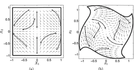
To add a degree of complexity to this analytical model, we introduce a rotation, thereby creating additional spatial variations. The rotation is a function of the ra-dial distance from the origin. Taking an initial set of points (X1, X2) in their polar
coordinate form (r cos 9, r sin 9), and increasing 9 with radial distance gives:
x, = r cos(9
+
r) = r (cos(9) cos(r) - sin(9) sin(r)) = r -, cos(r) - -2 sin(r)),(r r
= X1 cos(r) - X2 sin(r),
X2 = r sin(9
+
r) = r (sin(0) cos(r)+
cos(0) sin(r)) = r(2
cos(r)+
-l sin(r)),(r r = X2 cos(r) + X1 sin(r), (2.4) where r = fx 12 ± x2 2 = VX1 2
± X22 because no deformation in the radial direction has been made. A velocity field of the transformed system is presented in figure
2-1 0.5 0 -0.5 -1 -1 -0.5 0 X1 0.5 1 0.5 Or"~ NA / 7\ /7-7 -1 -0.5 0 X1 0.5 1 (a) (b)
Figure 2-2: Velocity field and sample trajectories of the system in (a) equation (2.2) and (b) equation (2.5). The trajectories (red lines) originate from their starting positions (circles) and extend to their final positions (crosses) over the time interval t = [0 2].
2(b).
The equations of motion for the transformed coordinates are calculated by taking the time derivative of equation (2.4):
= - X2
#)
cos(r) - (k 2 &2 = (k1 - X2?)
sin(r)+
(k 2where it can be shown that
± X17) sin(r),
± x1p) cos(r),
.X1k1
+
X2r2r = 2
Iv/X1'+ X2'
and the equations of motion (2.2) are substituted back in. Finally, we seek an ana-lytical expression for the velocity field in terms of the new (XI, x2) coordinates, which
is obtained by the substitution:
X1 = X1cos(r) + x2sin(r),
X2 = X2cos(r) - x, sin(r), (2.7)
into equations (2.2), (2.5), and (2.6). Solutions for the transformed equations of -0.5 -1 At . -(2.5) (2.6) 1
motion in equation (2.5) with the initial position (a,, a2) coordinates are:
xi(t, a,, a2) = X 1(t, A1(ai, a2)) cos (r(t, ai, a2))
- X2(t, A2(al, a2)) sin (r(t, a,, a2)),
x2 (t, ai, a2) = X2(t, A2(ai, a2)) cos (r(t,
a,,
a2))+ X, (t , (a, , a2)) Sin (r(t, a,, a2)). (2.8)
2.2.2
Non-Autonomous System: Double-Gyre
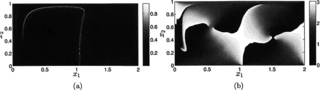
The analytic, time-dependent velocity field that we use as our example of a non-autonomous system is the well-known double-gyre system (Shadden et al., 2005). It is a simplification of the double-gyre features that are produced frequently in geophysical systems (Coulliette & Wiggins, 2001). Qualitatively, this system consists of two counter rotating gyres that oscillate in size and are contained within a domain with slip at the no-flux walls. The equations of motion for the double-gyre are:
,1 = -rA sin(7rf(xi, t)) cos(=rx2),
i2 = 7rA cos(rf (xi, t)) sin(7rX2)
d,
(2.9)where A is a scalar that sets the characteristic flow speed of the system, and
f(xi, t) = a(t)X12 + b(t)xi,
a(t) = csin(wt), b(t) = 1 - 2esin(wt),
c being the degree to which the gyres oscillate from side to side, and W being the
frequency of gyre oscillation. The system is defined in the domain D = {xi E
[0 2], yi E [0 1]}. For the examples in this chapter, we will use the parameters
A = 0.1,E = 0.1, and w = 27r/10. Snapshots of the corresponding velocity field are
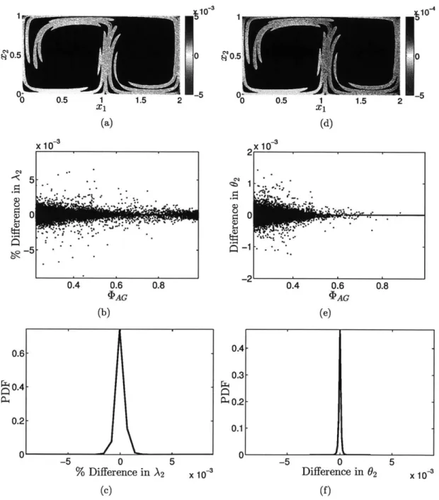
![Figure 2-10: (a) FTLE and (b) 02 based on equation (2.21) for the time interval t = [0 2] and calculated by the AG method](https://thumb-eu.123doks.com/thumbv2/123doknet/14723808.571215/47.918.199.686.140.355/figure-ftle-based-equation-time-interval-calculated-method.webp)
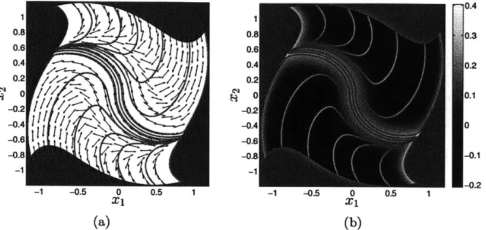
![Figure 2-18: The positive (a) and negative (b) shearlines for the double-gyre system the FTLE field for the time window t = [0 10]](https://thumb-eu.123doks.com/thumbv2/123doknet/14723808.571215/60.918.134.753.135.305/figure-positive-negative-shearlines-double-ftle-field-window.webp)