HAL Id: hal-03093363
https://hal.archives-ouvertes.fr/hal-03093363
Preprint submitted on 3 Jan 2021
HAL is a multi-disciplinary open access
archive for the deposit and dissemination of
sci-entific research documents, whether they are
pub-lished or not. The documents may come from
teaching and research institutions in France or
abroad, or from public or private research centers.
L’archive ouverte pluridisciplinaire HAL, est
destinée au dépôt et à la diffusion de documents
scientifiques de niveau recherche, publiés ou non,
émanant des établissements d’enseignement et de
recherche français ou étrangers, des laboratoires
publics ou privés.
First Co-spatial Comparison of Stellar, Neutral-, and
Ionized-gas Metallicities in a metal-rich galaxy: M83
Svea Hernandez, Alessandra Aloisi, Bethan L. James, Nimisha Kumari,
Danielle Berg, Angela Adamo, William P. Blair, Claude-André
Faucher-Giguère, Andrew J. Fox, Alexander B. Gurvich, et al.
To cite this version:
Svea Hernandez, Alessandra Aloisi, Bethan L. James, Nimisha Kumari, Danielle Berg, et al.. First
Co-spatial Comparison of Stellar, Neutral-, and Ionized-gas Metallicities in a metal-rich galaxy: M83.
2021. �hal-03093363�
FIRST CO-SPATIAL COMPARISON OF STELLAR, NEUTRAL-, AND IONIZED-GAS METALLICITIES IN A
METAL-RICH GALAXY: M83∗
Svea Hernandez,1Alessandra Aloisi,2 Bethan L. James,1 Nimisha Kumari,1 Danielle Berg,3 Angela Adamo,4 William P. Blair,5Claude-Andr´e Faucher-Gigu`ere,6 Andrew J. Fox,1 Alexander B. Gurvich,7 Zachary Hafen,8
Timothy M. Heckman,9 Vianney Lebouteiller,10 Knox S. Long,2, 11 Evan D. Skillman,12Jason Tumlinson,2, 9 and Bradley C. Whitmore2
1AURA for ESA, Space Telescope Science Institute, 3700 San Martin Drive, Baltimore, MD 21218, USA 2Space Telescope Science Institute, 3700 San Martin Drive, Baltimore, MD 21218, USA
3The Ohio State University, 4061 McPherson Chemical Laboratory, 140 W 18th Ave., Columbus, OH 43210
4Department of Astronomy, Oskar Klein Centre, Stockholm University, AlbaNova University Centre, SE-106 91 Stockholm, Sweden 5Department of Physics and Astronomy, The Johns Hopkins University, 3400 N. Charles Street, Baltimore, MD 21218
6Department of Physics and Astronomy, Northwestern University, 2145 Sheridan Road, Evanston, IL 60208-3112 7Department of Physics & Astronomy and CIERA, Northwestern University, 1800 Sherman Ave, Evanston, IL 60201, USA 8Department of Physics and Astronomy and Center for Interdisciplinary Exploration and Research in Astrophysics (CIERA),
Northwestern University, 2145 Sheridan Road, Evanston, IL 60208, USA
9Center for Astrophysical Sciences, Department of Physics and Astronomy, The Johns Hopkins University, Baltimore, MD 21218, USA 10AIM, CEA, CNRS, Universit´e Paris-Saclay, Universit´e Paris Diderot, Sorbonne Paris Cit´e, F-91191 Gif-sur-Yvette, France
11Eureka Scientific, Inc. 2452 Delmer Street, Suite 100, Oakland, CA 94602-3017, USA
12Minnesota Institute for Astrophysics, School of Physics and Astronomy, 116 Church Street S.E., University of Minnesota, Minneapolis,
MN 55455, USA (Accepted December 25, 2020)
Submitted to ApJ ABSTRACT
We carry out a comparative analysis of the metallicities from the stellar, neutral-gas, and ionized-gas components in the metal-rich spiral galaxy M83. We analyze spectroscopic observations taken with the Hubble Space Telescope (HST), the Large Binocular Telescope (LBT) and the Very Large Telescope (VLT). We detect a clear depletion of the HIgas, as observed from the HIcolumn densities in the nuclear region of this spiral galaxy. We find column densities of log[N (HI) cm−2] < 20.0 at galactocentric distances of < 0.18 kpc, in contrast to column densities of log[N (HI) cm−2]∼ 21.0 in the galactic disk, a trend observed in other nearby spiral galaxies. We measure a metallicity gradient of −0.03 ± 0.01 dex kpc−1for the ionized gas, comparable to the metallicity gradient of a local benchmark
of 49 nearby star-forming galaxies of−0.026 ± 0.002 dex kpc−1. Our co-spatial metallicity comparison of the multi-phase gas and stellar populations shows excellent agreement outside of the nucleus of the galaxy hinting at a scenario where the mixing of newly synthesized metals from the most massive stars in the star clusters takes longer than their lifetimes (∼10 Myr). Finally, our work shows that caution must be taken when studying the metallicity gradient of the neutral-gas component in star-forming galaxies, since this can be strongly biased, as these environments can be dominated by molecular gas. In these regions the typical metallicity tracers can provide inaccurate abundances as they may trace both the neutral- and molecular-gas components.
Keywords: galaxies – abundances – ISM – starburst
Corresponding author: Svea Hernandez
sveash@stsci.edu
∗Based on observations made with the Hubble Space Telescope
under program ID 14681.
2 Hernandez et al.
1. INTRODUCTION
Understanding the formation and evolution of galax-ies continues to be one of the main quests in modern astrophysics. Extragalactic abundance measurements have greatly contributed to uncover a variety of phys-ical and evolutionary processes influencing events tak-ing place within and among galaxies. Studies of galac-tic gradients and global metallicity relations (i.e., mass-metallicity relation, MZR) are widely used to investigate star-formation episodes, galactic winds, and accretion of pristine matter (Searle 1971; McCall et al. 1985; Zarit-sky et al. 1994;Tremonti et al. 2004;Andrews & Martini 2013;Kudritzki et al. 2015).
The measurements from both the MZR and metallic-ity trends in star-forming galaxies (SFGs), have relied for decades on the analysis of emission lines from H II
regions. Typically, when inferring the gas-phase metal-licities from the most common heavy element, oxygen, two main techniques are applied: strong-line analysis, and the electron temperature based (Te-based) method.
The strong-line analysis is based on the flux ratios of some of the strongest forbidden lines, e.g., [O II] and [OIII], with respect to hydrogen (Pagel et al. 1979; Mc-Gaugh 1994). On the other hand, the “direct” method, or Te-based method, relies on the flux ratio of
auro-ral to nebular lines, e.g., [OIII] λ4363/[O III] λλ4959, 5007, to measure the temperature of the high-excitation zone (Dinerstein et al. 1985; Rubin et al. 1994; Lee et al. 2004; Stasi´nska 2005). Furthermore, in the last decades these nebular techniques have been extended to studies of star-forming galaxies at high redshift (Pettini et al. 2001; Kobulnicky & Kewley 2004; Savaglio et al. 2005; Cowie & Barger 2008). Although the analysis of H II regions have made invaluable contributions when it comes to investigating the present-day chemical state of starburst galaxies, these regions could be enhanced compared to the surrounding interstellar medium (ISM, Kunth & Sargent 1986; Lebouteiller et al. 2013). And only in a few cases (e.g., S´anchez Almeida et al. 2015; Lagos et al. 2018) studies have found the metallicities in HIIregions to be lower than the rest of the galaxy. This has been attributed to infall of cold metal-poor gas.
An alternative method for investigating the chemical composition of galaxies is to directly study the neutral gas in SFGs. The metal content of a galaxy can be exam-ined through the analysis of the absorption lines in their far ultraviolet (UV) spectroscopic observations. A com-mon technique is to use bright UV targets within these galaxies as background sources (Kunth et al. 1994). In such observations, the metals along the line of sight im-print absorption features on the UV continuum of such targets. This technique has been applied extensively to
local galaxies (Aloisi et al. 2003;Lebouteiller et al. 2013; Werk et al. 2013;James et al. 2014). This approach not only allows us to study the metal contents accounting for the bulk of the mass of the galaxy, it also provides us with a view of the metal enrichment over large spatial scales and long timescales (dilution of abundances in HI
regions).
A third approach to studying the metallicities of star-forming galaxies is the analysis of young stellar popu-lations or individual stars. New techniques have been developed in the last decade to investigate the chemi-cal contents of nearby galaxies using blue supergiants, BSGs, and red supergiants, RSGs, as metallicity trac-ers (Davies et al. 2010, 2015, 2017a,b; Kudritzki et al. 2012, 2013, 2014; Hosek et al. 2014). Additionally, it is also possible to measure stellar metallicities from integrated-light spectroscopic observations of star clus-ters in nearby galaxies using high-resolution observa-tions (Colucci et al. 2011,2012;Larsen et al. 2006,2008, 2012,2014,2017,2018). This same technique has most recently been extended to intermediate-resolution obser-vations of extragalactic stellar populations (Hernandez et al. 2017,2018a,b,2019) as well as for populations at high redshifts (Halliday et al. 2008; Steidel et al. 2016; Chisholm et al. 2019).
In spite of the variety of tools available to investi-gate the chemical composition of star-forming galax-ies, detailed comparisons of the abundances obtained from the ionized-gas, neutral-gas, and stellar compo-nents are needed to fully understand the chemical state and evolution of galaxies. The general expectation is that young populations of stars should have a similar chemical composition as their parent gas cloud and as-sociated H II region. In this context, several studies in low-metallicity and chemically homogenous environ-ments have shown agreement between the ionized-gas and young stellar population metallicities (Bresolin et al. 2006;Lee et al. 2006). Studies of different galaxies with higher metallicities, such as spiral galaxies, have shown a varying degree of agreement between their nebular and stellar metallicities, from excellent (<0.1 dex) to differences as high as ∼0.2 dex (Bresolin et al. 2009, 2016; Hosek et al. 2014; Davies et al. 2017b). Even more intriguing is the fact that different studies have also hinted that for high-metallicity environments the Te-based method underestimates the metallicities; this
is suggested when compared to stellar abundances ( Zu-rita & Bresolin 2012; Sim´on-D´ıaz & Stasi´nska 2011; Garc´ıa-Rojas et al. 2014). These high-metallicity en-vironments are particularly challenging to study as the application of the direct method is limited given that
the temperature-sensitive lines are typically too weak to be detected (Bresolin et al. 2005).
Studies comparing different metallicity diagnostics show conflicting results. Through a study of 30 SFGs at z∼2, Steidel et al. (2016) found a factor of ∼4-5 difference between their inferred stellar and nebular metallicities, with a clear enhancement in the metallici-ties of the ionized gas. They argue that these artificially low stellar metallicities are observed due to the super-solar α/Fe abundance ratios of these galaxies at z∼2. They assume that this behavior is expected at high red-shift, and might be rare in low-z environments due to systematic differences in the star-formation history of typical galaxies. In a more recent study,Chisholm et al. (2019) measure the metallicity of these same compo-nents, ionized-gas and stellar, in a sample of 61 SFGs at z <0.2, and 19 galaxies at z∼ 2. In contrast to the work by Steidel et al. (2016), Chisholm et al. (2019) conclude that the stellar and nebular metallicities are similar to each other when assuming mixed-age stellar populations. Under the general assumption that young stellar populations have a similar chemical composition as their parent gas cloud and associated H II region, the work byChisholm et al. (2019) hints at a scenario where the gas surrounding high-mass stars is not instan-taneously metal-enriched by massive stars. This would imply that increasing the metallicity of the adjacent interstellar gas takes longer than the inferred lifetimes (∼10 Myr) of the massive stellar populations.
In this paper we analyze observations from the Cosmic Origin Spectrograph (COS) on Hubble, as well as data from the Multi-Object Double Spectrograph (MODS) on the Large Binocular Telescope (LBT) and the Multi Unit Spectroscopic Explorer (MUSE) on the Very Large Telescope (VLT) for a sample of pointings distributed across the face of the metal-rich spiral galaxy M83 (NGC 5236). M83 is our nearest face-on grand-design spiral and starburst galaxy (Dopita et al. 2010) at a distance of 4.9 Mpc (Jacobs et al. 2009, derived from the mag-nitudes of the tip of the red giant branch, TRGB). Its proximity and orientation allow for a spatially resolved study of its different components: stellar, neutral gas, and ionized gas. We present in Table1a detailed list of the general parameters of M83. Our main motivation is to understand how abundances from the different galaxy components relate to each other, particularly in a chal-lenging environment as is the metal-rich regime. In Sec-tion2we describe the observations and data reduction. The analysis of the different observations and for the different metallicity components is detailed in Section 3. We discuss our findings in Section4, and provide our concluding remarks in Section5.
Table 1. General parameters for M83
Parameter Value
R.A. (J2000.0) 204.253958◦ Dec (J2000.0) -29.865417◦
Distancea 4.9 Mpc
Morphological type SAB(s)c
R25b 6.440 (9.18 kpc)
Inclinationb 24◦
Position Anglec 45◦
Heliocentric radial velocity 512.95 km s−1 Notes. All parameters from the NASA Extragalactic Database (NED), except where noted.
aJacobs et al.(2009) b
de Vaucouleurs et al.(1991)
cComte(1981)
2. OBSERVATIONS AND DATA REDUCTION
2.1. COS observations
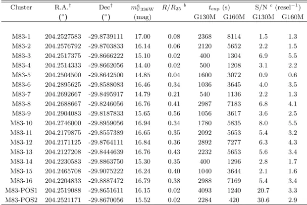
The analysis done here relies on the observations taken as part of HST program ID (PID) 14681 (PI: Aloisi), collected between 2017 May–July. The targets were ac-quired using near-UV (NUV) imaging, and the spec-troscopic data were observed with the G130M/1291 and G160M/1623 settings returning wavelength cover-age from 1130 to 1800 ˚A. The data were collected at Lifetime Position 3 providing a wavelength-dependent resolution ranging between R∼15,000 and 20,000. The targets observed in HST program ID 14681 were cho-sen from the list of young star clusters in the Wide Field Camera 3 (WFC3) Early Release Science Cycle 17 GO/DD PID 11360 (PI: O’Connell) and Cycle 19 GO PID 12513 (PI: Blair). An overview of this WFC3 multi-wavelength campaign is provided inBlair et al.(2014). Our selection criterion required targets to have magni-tudes mF336W. 17. We list in Table2the properties of
our COS sample along with the information of their ob-servations. We note that the spectroscopic observations for the M83-5 pointing were affected by a guide star fil-ure after the science exposfil-ures began collecting data. This caused the S/N of the resulting spectroscopic data for this target to be lower than originally planned. For this reason we have excluded this target from our anal-ysis.
In addition to the targets from PID 14681, we ex-tended our analysis to include two more COS point-ings, M83-POS1 and M83-POS2, observed as part of HST PIDs 11579 and 15193 (PI: Aloisi). These addi-tional observations were taken using the G130M/1291 and G160M/1623 setting with similar wavelength
cov-4 Hernandez et al. erage as that from PID 14681. Our final COS sample
is composed of 17 pointings distributed throughout the disk of M83 as indicated in Figure1.
We retrieved the observations from the Mikulski Archive for Space Telescopes (MAST) and calibrated them using the HST pipeline, CALCOS v3.3.4 (Fox et al. 2015). More details on the reduction of the ob-servations are provided byHernandez et al. (2019). As a final step we bin the spectra by a COS resolution ele-ment (1 resel = 6 pixels), corresponding to the nominal point-spread function.
2.2. MODS observations
Optical spectra of the H II regions in M83 were ac-quired with MODS (Pogge et al. 2010) on the LBT on the UT date of 2018 May 21. The primary goal was to obtain high signal-to-noise spectra, with detections of the intrinsically faint auroral lines (e.g., [O III] λ4363, [NII] λ5755, [SIII] λ6312), in order to obtain accurate abundances of the gas surrounding the ionizing young massive clusters (YMCs) observed with COS and pre-sented by Hernandez et al. (2019). To do so, we used the multi-object mode of MODS, which uses custom-designed, laser-milled slit masks, allowing multiple HII
regions to be targeted simultaneously. We highlight that two masks were originally cut to cover the whole COS sample. However, due to poor weather conditions and other complications, only half of the data were collected. The M83 mask used, which targets 13 H II regions si-multaneously, was observed for three exposures of 1200s, or a total integration time of 1-hour. At the latitude of the LBT, M83 stays below 30◦ on the sky, and thus
the observations were obtained at relatively high air-mass (∼2–3). To compensate, slits were cut close to the median parallactic angle of the observing window (PA=0), minimizing flux lost due to differential atmo-spheric refraction between 3200 – 10,000 ˚A (Filippenko 1982). Blue and red spectra were obtained simultane-ously using the G400L (400 lines mm−1, R ∼ 1850) and G670L (250 lines mm−1 R ∼ 2300) gratings, re-spectively. The resulting combined spectra extend from 3200–10000 ˚A, with a resolution of∼ 2 ˚A(FWHM).
Broad R-band and continuum-subtracted Hα images of M83 from The Spitzer Local Volume Legacy Survey (LVL;Dale et al. 2009) were used to identify the sample of target H II regions, as well as the alignment stars. H II regions were selected by prioritizing the knots of high Hα surface brightness that are in the closest phys-ical proximity to the YMCs. All target slits are 1.000 wide, but with lengths varying according to the size of each H II region. The resulting multi-slit mask con-tained 13 H II region slits and 2 sky slits. We list in
the Appendix in Table9 the coordinates of each of the slits. The mask slit locations are shown in Figure1 in comparison to the stellar clusters. Within the slit mask footprint, and avoiding aberration issues near the edges, we were able to target six distinct HII regions that di-rectly correspond to YMC regions. To effectively use the mask real estate, we targeted six additional HIIregions that do not clearly correspond to one the of YMCs (R4, R5, R9, R13, R14, and R15).
The M83 optical spectra were reduced and analyzed using the MODS reduction pipeline1following the proce-dures detailed inBerg et al.(2015). Here, we summarize notable reduction steps. Given the crowding of bright HIIregions in the disk of M83, diffuse nebular emission can complicate local sky subtraction. Therefore, the ad-ditional sky slits cut in the mask were used to provide a basis for clean sky subtraction. Continuum subtrac-tion was performed in each slit by scaling the continuum flux from the sky-slit to the local background continuum level. One-dimensional spectra were then corrected for atmospheric extinction and flux calibrated based on ob-servations of flux standard stars (Bohlin 2014).
2.3. MUSE observations
To complement our COS and MODS observations we make use of archival MUSE data covering 12 out of 17 clusters in our COS sample with spectral resolution in-creasing between R ∼ 1770 at the bluest wavelengths (4800 ˚A) and R∼ 3590 at the reddest wavelengths (9300 ˚
A). The observations were taken during 2016 April and 2017 April–May as part of PID: 096.B-0057(A) with PI: Adamo. We downloaded the fully reduced dat-acubes from the European Southern Observatory (ESO) archive. The datacubes are reduced using the MUSE pipeline v.2.0.1, which performs removal of instrumental artifacts, astrometric calibration, sky-subtraction, wave-length and flux calibrations. We note that upon further inspection we found that the astrometric calibration for these archival datacubes was not correct, so we man-ually corrected their astrometry through a comparison with HST images.
We identify the location of the 12 clusters in our COS sample within the MUSE cubes and extract their spec-tra. The extraction was done by summing all spec-tra within circular apertures of diameter 2.500 co-spatial with the HST/COS pointings, taking into account the fractional level of overlap of the spatial pixel with the region. We identified a few bad pixels in the datacubes and excluded them from our analysis. In the left panel
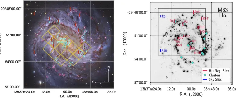
13h37m24.0s 12.0s 00.0s 36m48.0s 36.0s -29 48’00.0” 51’00.0” 54’00.0” 57’00.0” R.A. (J2000) Dec. (J2000)
M83
H↵
R1 R2 R4 R5 R6 R7 R8 R9 R11 R12 R13 R14 R15 R3 R10Hii Reg. Slits Clusters Sky Slits 13h37m24.0s 12.0s 00.0s 36m48.0s 36.0s -2948’00.0” 51’00.0” 54’00.0” 57’00.0” R.A. (J2000)
R-Band
C1 C2 C3 C4 C5 C6 C7 C8 C9 C10 C11 C12 C13 C14 C15 C16Figure 1. Lef t: Color-composite image observed with the 2.2m Max Planck-ESO Telescope, the 8.2m Subaru Telescope (NAOJ), and the Hubble Space Telescope. We marked with cyan circles the location of the star clusters observed with COS. We overlay the footprints of the MODS slits in red showing the position of the observed HIIregions. MUSE FoV are shown in yellow. Processing and Copyright: Robert Gendler. Right: Spitzer Local Volume Legacy Survey Hα image of M83 (Dale et al. 2009). The footprint of the LBT/MODS mask is shown as a gray square, with sky slits (blue) and HIIregion slit locations (red) overlaid in comparison to the stellar clusters targeted with COS (cyan diamonds). The slit positions targeted HIIregions associated with YMCs, although additional associated HIIregions were added in order to maximize effective usage of mask real estate.
of Figure 1 we highlight in yellow the fields of view of MUSE.
3. ANALYSIS
3.1. Neutral-gas Metallicities 3.1.1. Continuum and line-profile fitting
As part of the analysis performed we normalized the individual COS spectroscopic observations before fitting the different line profiles. We fit the continuum of the star clusters by interpolating between regions (nodes) strategically positioned to avoid stellar and ISM absorp-tion. We make use of a spline function when interpolat-ing between the manually defined nodes.
We derive the column densities for the different el-ements by fitting Voigt profiles using the recently de-veloped Python software VoigtFit v.0.10.3.3 (Krogager 2018). This relatively new code allows users to pro-vide line spread function (LSF) tables to account for the broadening of the absorption lines introduced by the instrument itself. We convolve the COS LSF profiles with the FWHM of the source in the dispersion direc-tion as measured from the acquisidirec-tion images, similar to the approach described in Section 3.3 in Hernandez et al. (2020). We also note that VoigtFit allows for multi-component fitting, particularly useful for deblend-ing different components along the same line of sight.
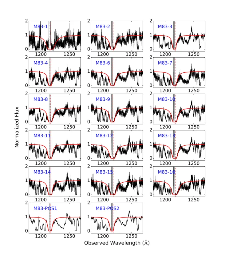
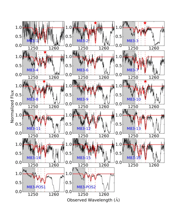
We note that although the COS observations allow us to access a variety of absorption lines of several heavy elements, our work focuses on measuring the metallicity of the neutral gas. Given that S/H traces metallicity reliably (Lebouteiller et al. 2013;James & Aloisi 2018) we primarily study the SIIand Lyα lines. We present in Table3 the theoretical parameters for each of the lines analyzed as part of this work. We show in Figures2and 3the best fitting profiles for the Lyman α and SIIlines along with the COS observations.
3.1.2. HI
The COS observations analyzed here cover the Lyα absorption line at λ =1215.671 ˚A originating from the multiple sightlines in M83. Given the close proximity of M83, the Lyα absorption from the MW is heavily blended with those from our M83 pointings. In order to extract precise column densities for the HIgas in M83 we simultaneously fit the MW and galaxy Lyα profiles. Following the approach adopted byJames et al.(2014), we make use of the red wing of Lyα to constrain the fit of the H I column density intrinsic to the different targets, and adopt a fixed MW HIcolumn density mea-sured in James et al. (2014) in the direction of M83, log[N (H I)MW cm−2] = 20.57. Measurements of the
HIcolumn densities of the individual pointings in M83, log[N (H I)], are listed in Table 4. Lastly, the best
fit-6 Hernandez et al.
0.0
0.2
0.4
0.6
0.8
1.0
Observed Wavelength (
Å
)
0.0
0.2
0.4
0.6
0.8
1.0
Normalized Flux
1200
1250
0
1
2
M83-1
1200
1250
0
1
2
M83-2
1200
1250
0
1
2
M83-3
1200
1250
0
1
2
M83-4
1200
1250
0
1
2
M83-6
1200
1250
0
1
2
M83-7
1200
1250
0
1
2
M83-8
1200
1250
0
1
2
M83-9
1200
1250
0
1
2
M83-10
1200
1250
0
1
2
M83-11
1200
1250
0
1
2
M83-12
1200
1250
0
1
2
M83-13
1200
1250
0
1
2
M83-14
1200
1250
0
1
2
M83-15
1200
1250
0
1
2
M83-16
1200
1250
0
1
2
M83-POS1
1200
1250
0
1
2
M83-POS2
Figure 2. Lyα profiles for the M83 pointings in our sample. In black we show the COS observations binned by 1 resolution element (1 resel = 6 pixels). In red we display the best fitting VoigtFit model. The names of the individual targets are shown in each panel. We show with thin dashed lines the MW component (grey) and the M83 component (red).
Table 2. Properties of the observed targets and their COS Observations
Cluster R.A.† Dec† ma
F336W R/R25 b texp (s) S/Nc(resel−1) (◦) (◦) (mag) G130M G160M G130M G160M M83-1 204.2527583 -29.8739111 17.00 0.08 2368 8114 1.5 1.3 M83-2 204.2576792 -29.8703833 16.14 0.06 2120 5652 2.2 1.5 M83-3 204.2517375 -29.8666222 15.10 0.02 400 1304 6.9 5.5 M83-4 204.2514333 -29.8662056 14.40 0.02 500 1208 3.1 2.2 M83-5 204.2504500 -29.8642500 14.85 0.04 1600 3072 0.9 0.6 M83-6 204.2895625 -29.8588083 16.46 0.34 1036 3645 4.0 3.5 M83-7 204.2692667 -29.8495917 14.79 0.21 540 1136 2.2 1.3 M83-8 204.2688667 -29.8246056 16.76 0.41 2987 7183 6.8 4.1 M83-9 204.2904083 -29.8187833 15.65 0.56 1056 3617 3.6 2.5 M83-10 204.2746000 -29.8959056 16.94 0.34 1780 5835 8.0 5.5 M83-11 204.2179875 -29.8557389 16.65 0.35 2092 5653 5.4 3.2 M83-12 204.2171125 -29.8764111 16.84 0.36 2892 7277 6.3 4.3 M83-13 204.2127208 -29.8444639 16.76 0.43 2232 5653 5.6 3.4 M83-14 204.2230583 -29.8863750 15.30 0.35 400 1296 2.8 1.7 M83-15 204.2465708 -29.9075222 16.24 0.40 1040 3644 2.1 1.6 M83-16 204.2204833 -29.8887472 16.79 0.38 2988 7169 5.4 3.4 M83-POS1 204.2519088 -29.8651611 16.15 0.02 4093 1240 20.7 3.3 M83-POS2 204.2521171 -29.8670056 15.52 0.02 2284 420 30.6 2.9 †
Coordinates extracted from the Mikulski Archive at the Space Telescope Science Institute (MAST). We note that the HST performance has jitter of 0.00800 RMSd.
a
Magnitudes are in the Vegamag system, calculated using a 2.500 aperture size.
b
Calculated adopting the parameters listed in Table1.
c
Estimated at wavelengths of 1310 ˚A and 1700 ˚A for G130M and G160M, respectively.
8 Hernandez et al.
0.0
0.2
0.4
0.6
0.8
1.0
Observed Wavelength (
Å
)
0.0
0.2
0.4
0.6
0.8
1.0
Normalized Flux
1250
1260
0.0
0.5
1.0
M83-1
1250
1260
0.0
0.5
1.0
M83-2
1250
1260
0.0
0.5
1.0
M83-3
1250
1260
0.0
0.5
1.0
M83-4
1250
1260
0.0
0.5
1.0
M83-6
1250
1260
0.0
0.5
1.0
M83-7
1250
1260
0.0
0.5
1.0
M83-8
1250
1260
0.0
0.5
1.0
M83-9
1250
1260
0.0
0.5
1.0
M83-10
1250
1260
0.0
0.5
1.0
M83-11
1250
1260
0.0
0.5
1.0
M83-12
1250
1260
0.0
0.5
1.0
M83-13
1250
1260
0.0
0.5
1.0
M83-14
1250
1260
0.0
0.5
1.0
M83-15
1250
1260
0.0
0.5
1.0
M83-16
1250
1260
0.0
0.5
1.0
M83-POS1
1250
1260
0.0
0.5
1.0
M83-POS2
Figure 3. SIIprofiles for the M83 pointings in our sample. In black we show the COS observations binned by 1 resolution element (1 resel = 6 pixels). In red we display the best fitting model. The names of the individual targets are shown in each panel. Vertical grey dashed lines show the location of the MW components, vertical red dashed lines indicate the strongest M83 components. We note that we have masked out the MW SIIλ1250 line when fitting our extragalactic SIIlines, as this is strongly affected by the P-Cygni profile of the NVline. We show these masks as shaded grey regions. Lastly, we mark those pointings exhibiting hidden saturation with a red F. The fits for these targets have been obtained excluding the strongest SII λ1253 line.
Table 3. Atomic Data for UV absorption lines Line ID λrest fa (˚A) Lyα 1215.6710 4.16e-01 SII 1250.5780 5.43e-03 SII 1253.8050 1.09e-02 a
Oscillator strength values compiled by the Vienna Atomic Line Database 3 (VALD3).
ting profiles for the whole sample are shown in different panels in Figure2.
3.1.3. SII
In general, direct measurements of the oxygen abun-dances in the neutral gas are difficult to access as the most easily observed OIline, 1302 ˚A, in the COS spec-tral coverage at low redshifts is typically saturated. On the other hand, OIat 1355 ˚A is too weak to be detected. As such, we use proxies for oxygen to indirectly derive the oxygen abundances (James & Aloisi 2018). As part of our analysis we measure the column densities of the S II lines listed in Table 3 and make use of the solar ratio of log(S/O) = −1.57 ± 0.06 to derive the O/H
abundances in the neutral gas of M83. 3.1.4. Curve-of-growth Analysis
To assess if our measured abundances are affected by saturation, we plot the column density measurements along the curve-of-growth (COG) corresponding to the ion in question. For each ion we generate a COG show-ing the relation between the equivalent width, log(W/λ), and the column density, log(f N ), where f is the oscilla-tor strength. When generating the individual COGs we adopt the b parameters listed in Appendix Bin Table 10 inferred from the simultaneous line-profile fitting of the SII lines.
In Figure 4 we show a selected sample of COGs il-lustrating the line strength regimes encountered in our analysis. We primarily use the location of the SII tran-sitions on their corresponding COG to determine if the column density estimates are reliable or if they need to be considered as lower limits due to saturation effects. For those pointings where both SIItransitions are found on the right side of the vertical line, we consider them as saturated lines as they occupy the curved or satu-rated regime in the COG (see left panel in Figure 4). In those cases we are unable to constrain the column densities for SII and we consider them as lower limits. We also identified cases where one of the two transitions was found borderline or clearly in the saturated regime
as shown in the middle panel of Figure4. In such sce-nario we are still able to constrain the column densities as we fit the weakest transition, i.e., SII λ1250, avoid-ing hidden saturation effects. Lastly, we observed cases where both transitions were located on the linear part of the COG clearly showing an absence of saturation for those pointings.
3.1.5. Ionization corrections
In ISM abundance studies it is critical to take into ac-count ionization effects due to contaminating ionized gas along the line of sight and/or contributing higher ioniza-tion ions present in the neutral gas, but not measured directly from the observations. Generating tailored pho-toionization models for a sample of nearby star-forming galaxies, Hernandez et al. (2020, hereafter H20) found ionization correction factors (ICFs) as high as∼0.7 dex in the neutral gas, clearly demonstrating the importance of precise ICFs. To accurately infer the chemical abun-dances of the neutral gas along the different pointings throughout M83, as part of this work we investigate the amount of ionized gas contaminating the neutral abun-dance measurements (ICFionized), as well as the amount
of higher ionization ions, compared to the dominant ion of a certain species in the HIgas (ICFneutral).
To accurately estimate the ionization effects affect-ing our measured abundances we adopt a similar ap-proach as that followed by H20. We generate tailored photoionization models for each of the pointings in our sample using the spectral synthesis code CLOUDY ( Fer-land et al. 2017). We adopt an overall metallicity of Z= 3.24 Z as measured from the ionized-gas component
(Marble et al. 2010). The work of H20 takes advan-tage of newly acquired COS/FUV observations covering bluer wavelengths than our M83 COS/FUV data, which they use to measure the FeIII/FeIIratio for the galax-ies in their sample, including two M83 pointings in our analysis here (M83-POS1 and M83-POS2). This ratio is a critical indicator of the gas volume density of the targets and is essential to generate tailored photoion-ization models. Given that the Fe IIIline at λ = 1122 ˚
A is not covered in our COS observations, we instead adopt an average value from the two M83 pointings in H20 of log[N (Fe III)/N (Fe II)] = −0.811 dex for the rest of the M83 targets studied here. Furthermore, H20 estimate the effective temperature of the star clusters observed in the two M83 pointings in their sample to be Teff =42,500 K. We adopt the same Teff for the rest of
our M83 pointings. We highlight that according to the work by H20, this physical parameter (Teff) has
mini-mal effects on the final ICF values calculated from the photoionization models. The rest of the input
param-10 Hernandez et al.
SII M83 1
7.0 7.5 8.0 8.5 9.0 9.5 10.0 log [Nf ] (log(cm1 )) 5.0 4.5 4.0 3.5 3.0 2.5 2.0 log (W/ )SII M83 2
7.0 7.5 8.0 8.5 9.0 9.5 10.0 log [Nf ] (log(cm1 )) 5.0 4.5 4.0 3.5 3.0 2.5 2.0 log (W/ )SII M83 2 2
7.0 7.5 8.0 8.5 9.0 9.5 10.0 log [Nf ] (log(cm1 )) 5.0 4.5 4.0 3.5 3.0 2.5 2.0 log (W/ )SII M83 3
7.0 7.5 8.0 8.5 9.0 9.5 10.0 log [Nf ] (log(cm1 )) 5.0 4.5 4.0 3.5 3.0 2.5 2.0 log (W/ )SII M83 4
7.0 7.5 8.0 8.5 9.0 9.5 10.0 log [Nf ] (log(cm1)) 5.0 4.5 4.0 3.5 3.0 2.5 2.0 log (W/ )SII M83 6
7.0 7.5 8.0 8.5 9.0 9.5 10.0 log [Nf ] (log(cm1)) 5.0 4.5 4.0 3.5 3.0 2.5 2.0 log (W/ )SII M83 7
7.0 7.5 8.0 8.5 9.0 9.5 10.0 log [Nf ] (log(cm1)) 5.0 4.5 4.0 3.5 3.0 2.5 2.0 log (W/ )SII M83 7 2
7.0 7.5 8.0 8.5 9.0 9.5 10.0 log [Nf ] (log(cm1)) 5.0 4.5 4.0 3.5 3.0 2.5 2.0 log (W/ )SII M83 8
7.0 7.5 8.0 8.5 9.0 9.5 10.0 log [Nf ] (log(cm1)) 5.0 4.5 4.0 3.5 3.0 2.5 2.0 log (W/ )SII M83 9
7.0 7.5 8.0 8.5 9.0 9.5 10.0 log [Nf ] (log(cm1)) 5.0 4.5 4.0 3.5 3.0 2.5 2.0 log (W/ )SII M83 10
7.0 7.5 8.0 8.5 9.0 9.5 10.0 log [Nf ] (log(cm1)) 5.0 4.5 4.0 3.5 3.0 2.5 2.0 log (W/ )SII M83 10 2
7.0 7.5 8.0 8.5 9.0 9.5 10.0 log [Nf ] (log(cm1)) 5.0 4.5 4.0 3.5 3.0 2.5 2.0 log (W/ )SII M83 11
7.0 7.5 8.0 8.5 9.0 9.5 10.0 log [Nf ] (log(cm1)) 5.0 4.5 4.0 3.5 3.0 2.5 2.0 log (W/ )SII M83 12
7.0 7.5 8.0 8.5 9.0 9.5 10.0 log [Nf ] (log(cm1)) 5.0 4.5 4.0 3.5 3.0 2.5 2.0 log (W/ )SII M83 13
7.0 7.5 8.0 8.5 9.0 9.5 10.0 log [Nf ] (log(cm1)) 5.0 4.5 4.0 3.5 3.0 2.5 2.0 log (W/ )SII M83 14
7.0 7.5 8.0 8.5 9.0 9.5 10.0 log [Nf ] (log(cm1)) 5.0 4.5 4.0 3.5 3.0 2.5 2.0 log (W/ )SII M83 1
7.0 7.5 8.0 8.5 9.0 9.5 10.0 log [Nf ] (log(cm1)) 5.0 4.5 4.0 3.5 3.0 2.5 2.0 log (W/ )SII M83 2
7.0 7.5 8.0 8.5 9.0 9.5 10.0 log [Nf ] (log(cm1)) 5.0 4.5 4.0 3.5 3.0 2.5 2.0 log (W/ )SII M83 2 2
7.0 7.5 8.0 8.5 9.0 9.5 10.0 log [Nf ] (log(cm1)) 5.0 4.5 4.0 3.5 3.0 2.5 2.0 log (W/ )SII M83 3
7.0 7.5 8.0 8.5 9.0 9.5 10.0 log [Nf ] (log(cm1)) 5.0 4.5 4.0 3.5 3.0 2.5 2.0 log (W/ )SII M83 4
7.0 7.5 8.0 8.5 9.0 9.5 10.0 log [Nf ] (log(cm1)) 5.0 4.5 4.0 3.5 3.0 2.5 2.0 log (W/ )SII M83 6
7.0 7.5 8.0 8.5 9.0 9.5 10.0 log [Nf ] (log(cm1)) 5.0 4.5 4.0 3.5 3.0 2.5 2.0 log (W/ )SII M83 7
7.0 7.5 8.0 8.5 9.0 9.5 10.0 log [Nf ] (log(cm1)) 5.0 4.5 4.0 3.5 3.0 2.5 2.0 log (W/ )SII M83 7 2
7.0 7.5 8.0 8.5 9.0 9.5 10.0 log [Nf ] (log(cm1)) 5.0 4.5 4.0 3.5 3.0 2.5 2.0 log (W/ )SII M83 8
7.0 7.5 8.0 8.5 9.0 9.5 10.0 log [Nf ] (log(cm1)) 5.0 4.5 4.0 3.5 3.0 2.5 2.0 log (W/ )SII M83 9
7.0 7.5 8.0 8.5 9.0 9.5 10.0 log [Nf ] (log(cm1)) 5.0 4.5 4.0 3.5 3.0 2.5 2.0 log (W/ )SII M83 10
7.0 7.5 8.0 8.5 9.0 9.5 10.0 log [Nf ] (log(cm1)) 5.0 4.5 4.0 3.5 3.0 2.5 2.0 log (W/ )SII M83 10 2
7.0 7.5 8.0 8.5 9.0 9.5 10.0 log [Nf ] (log(cm1)) 5.0 4.5 4.0 3.5 3.0 2.5 2.0 log (W/ )SII M83 11
7.0 7.5 8.0 8.5 9.0 9.5 10.0 log [Nf ] (log(cm1 )) 5.0 4.5 4.0 3.5 3.0 2.5 2.0 log (W/ )SII M83 12
7.0 7.5 8.0 8.5 9.0 9.5 10.0 log [Nf ] (log(cm1 )) 5.0 4.5 4.0 3.5 3.0 2.5 2.0 log (W/ )SII M83 13
7.0 7.5 8.0 8.5 9.0 9.5 10.0 log [Nf ] (log(cm1 )) 5.0 4.5 4.0 3.5 3.0 2.5 2.0 log (W/ )SII M83 14
7.0 7.5 8.0 8.5 9.0 9.5 10.0 log [Nf ] (log(cm1 )) 5.0 4.5 4.0 3.5 3.0 2.5 2.0 log (W/ )SII M83 14 2
7.0 7.5 8.0 8.5 9.0 9.5 10.0 log [Nf ] (log(cm1)) 5.0 4.5 4.0 3.5 3.0 2.5 2.0 log (W/ )SII M83 15
7.0 7.5 8.0 8.5 9.0 9.5 10.0 log [Nf ] (log(cm1)) 5.0 4.5 4.0 3.5 3.0 2.5 2.0 log (W/ )SII M83 15 2
7.0 7.5 8.0 8.5 9.0 9.5 10.0 log [Nf ] (log(cm1)) 5.0 4.5 4.0 3.5 3.0 2.5 2.0 log (W/ )SII M83 16
7.0 7.5 8.0 8.5 9.0 9.5 10.0 log [Nf ] (log(cm1)) 5.0 4.5 4.0 3.5 3.0 2.5 2.0 log (W/ )SII M83 POS1
7.0 7.5 8.0 8.5 9.0 9.5 10.0 log [Nf ] (log(cm1 )) 5.0 4.5 4.0 3.5 3.0 2.5 2.0 log (W/ )SII M83 POS1 2
7.0 7.5 8.0 8.5 9.0 9.5 10.0 log [Nf ] (log(cm1 )) 5.0 4.5 4.0 3.5 3.0 2.5 2.0 log (W/ )SII M83 POS2
7.0 7.5 8.0 8.5 9.0 9.5 10.0 log [Nf ] (log(cm1 )) 5.0 4.5 4.0 3.5 3.0 2.5 2.0 log (W/ )Figure 4. Selected sample of curves of growth displaying the linear and saturated regimes for a fitted b parameter specific to SII. We show with blue dashed lines the 1σ errors on the b parameter. We indicated with a dashed vertical line the transition from the linear to the saturated regime. Each subplot illustrates a different line-strength regime. The filled circles show the equivalent width, W , and column density, N , of each line as derived from our line-profile fitting analysis. Left: SIItransitions in the saturated part of the COG indicating saturation in both lines. Middle: One of the two transitions lies close to the saturated regime. The location of the second transition in the linear regime allows us to rule out the possibility of hidden saturation e.g., if we are able to fit both lines simultaneously. Right: Both transitions show unsaturated lines.
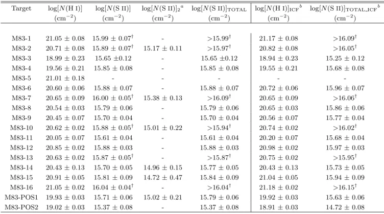
Table 4. Column densities for the different pointings in M83.
Target log[N (HI)] log[N (SII)] log[N (SII)]2a log[N (SII)]TOTAL log[N (HI)]ICFb log[N (SII)]TOTAL ICFb
(cm−2) (cm−2) (cm−2) (cm−2) (cm−2) (cm−2) M83-1 21.05 ± 0.08 15.99 ± 0.07† - >15.99† 21.17 ± 0.08 >16.09† M83-2 20.71 ± 0.08 15.89 ± 0.07† 15.17 ± 0.11 >15.97† 20.82 ± 0.08 >16.05† M83-3 18.99 ± 0.23 15.65 ±0.12 - 15.65 ±0.12 18.94 ± 0.23 15.25 ± 0.12 M83-4 19.56 ± 0.21 15.85 ± 0.08 - 15.85 ± 0.08 19.55 ± 0.21 15.68 ± 0.08 M83-5 21.01 ± 0.18 - - - - -M83-6 20.60 ± 0.06 15.88 ± 0.07 - 15.88 ± 0.07 20.72 ± 0.06 15.96 ± 0.07 M83-7 20.65 ± 0.09 16.00 ± 0.05† 15.38 ± 0.13 >16.09† 20.65 ± 0.09 >16.06† M83-8 20.54 ± 0.03 15.79 ± 0.06 - 15.79 ± 0.06 20.65 ± 0.03 15.86 ± 0.06 M83-9 20.45 ± 0.07 15.70 ± 0.04 - 15.70 ± 0.04 20.56 ± 0.07 15.77 ± 0.04 M83-10 20.62 ± 0.02 15.88 ± 0.05† 15.01 ± 0.22 >15.94† 20.74 ± 0.02 >16.02† M83-11 20.05 ± 0.07 15.61 ± 0.04 - 15.61 ± 0.04 20.20 ± 0.07 15.68 ± 0.04 M83-12 20.85 ± 0.02 15.88 ± 0.03 - 15.88 ± 0.03 20.98 ± 0.02 15.97 ± 0.03 M83-13 20.63 ± 0.02 15.87 ± 0.05† - >15.87† 20.75 ± 0.02 >15.95† M83-14 20.43 ± 0.13 15.70 ± 0.05 14.96 ± 0.15 15.77 ± 0.05 20.43 ± 0.13 15.73 ± 0.05 M83-15 20.91 ± 0.05 15.81 ± 0.09 14.72 ± 0.47 15.84 ± 0.09 21.04 ± 0.05 15.94 ± 0.09 M83-16 21.05 ± 0.02 16.04 ± 0.04† - >16.04† 21.18 ± 0.02 >16.15† M83-POS1 19.93 ± 0.03 15.71 ± 0.06 15.02 ± 0.21 15.79 ± 0.06 19.92 ± 0.03 15.63 ± 0.06 M83-POS2 19.02 ± 0.03 15.37 ± 0.08 - 15.37 ± 0.08 18.91 ± 0.03 14.72 ± 0.08
aMulti-component cases. A second SIIcomponent was identified for these pointings. b
Column densities calculated after applying the ionization correction factors listed in Table6. †
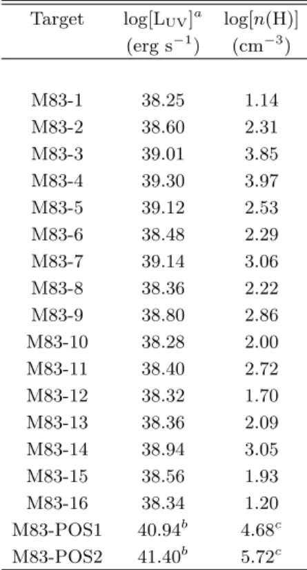
eters are listed in Table 5. We estimate the log[LUV]
values from the mF336W values listed in the Table 2,
with the exception of M83-POS1 and M83-POS2; the log[LUV] values for these two clusters were calculated
using ACS/SBC frames observed with the F125LP fil-ter. We measure the HIcolumn densities directly from the COS observations as described in section 4.1. In the third column of Table5 we show the measured vol-ume densities using the assvol-umed FeIII/FeIIratios. For more details on the precise steps taken to generate the photoionzation models we refer the reader toHernandez et al.(2020).
The different ICF values, ICFionized, ICFneutral, and
ICFTOTAL, for the full M83 sample are listed on Table
6. Similar to the work ofJames et al. (2014) and H20 we calculate the final column densities for each element X using the following equation:
log[N (X)ICF] = log[N (X)]− ICFTOTAL (1)
In Table6 we list the individual correction values, both ICFionizedand ICFneutral, for each ion and target. In the
last two columns of Table6we show the total ionization correction factors to be applied to the measured column densities. And finally, we list in the last columns of Table4 the ionization corrected column densities for H and S obtained after applying the inferred ICFTOTAL
using Equation1.
3.2. Nebular Metallicities
We measure the emission line fluxes from the optical observations (LBT and VLT) for the recombination and collisionally excited lines by fitting Gaussian profiles af-ter subtracting the continuum and absorption features in the spectral region of interest. Equal weight is given to the flux in each spectral pixel while fitting the Gaus-sian profiles. We further propagate the uncertainties on the three Gaussian parameters (amplitude, centroid, and FWHM) to estimate the final uncertainty in the fluxes.
We use the attenuation curve by Fitzpatrick et al. (2019) along with the observed Hα/Hβ ratio to esti-mate the nebular emission line color excess, E(B-V), at an electron temperature and density of 10,000 K and 100 cm−3, respectively (Case B recombination). We note that we have also tested our metallicity calculations assuming Case B recombination coefficients associated with an electron temperature of 5000 K (which may be more representative of the high metallicity gas within M83), and find that the final metallicity estimates are insensitive to the electron temperature adopted for the Case B recombination coefficient, within the uncertain-ties. The E(B-V) is then used to deredden the observed
Table 5. Input parameters for the CLOUDY models tailored to each of the M83 pointings in our sample
Target log[LUV]a log[n(H)]
(erg s−1) (cm−3) M83-1 38.25 1.14 M83-2 38.60 2.31 M83-3 39.01 3.85 M83-4 39.30 3.97 M83-5 39.12 2.53 M83-6 38.48 2.29 M83-7 39.14 3.06 M83-8 38.36 2.22 M83-9 38.80 2.86 M83-10 38.28 2.00 M83-11 38.40 2.72 M83-12 38.32 1.70 M83-13 38.36 2.09 M83-14 38.94 3.05 M83-15 38.56 1.93 M83-16 38.34 1.20 M83-POS1 40.94b 4.68c M83-POS2 41.40b 5.72c a
Luminosities estimated from the mF336W listed in Table2. bLuminosities estimated from the ACS/SBC frames
observed with the F125LP filter (Hernandez et al. 2020).
c
Volume densities fromHernandez et al. (2020).
emission line fluxes. We include in Appendix Cthe ta-bles listing the individual fluxes, dereddened fluxes and reddening values for each of the pointings studied here. As part of our analysis we tested various diagnos-tics for estimating the gas-phase metallicities, which in-cluded R232, O3N23, and N24 (Pettini & Pagel 2004;
Curti et al. 2017). We note that theCurti et al.(2017) metallicity calibrations are only valid for 12+log(O/H) < 8.85, objects with metallicities of 12+log(O/H) = 8.85 need to be considered lower limits. This limitation dras-tically reduced the number of available metallicity mea-surements in our study, as we are primarily exploring a high-metallicity environment. In a previous metallic-ity study of M83 by Bresolin et al. (2016), they find that empirically calibrated strong-line diagnostics usu-ally provide lower abundances than those inferred from the stellar populations. They attribute this behavior to
2([OII] λ3727+[OIII] λλ4959, 5007)/Hβ 3([OIII] λ5007/Hβ)/([NII] λ6584/Hα) 4[NII] λ6584/Hα
12 Hernandez et al.
Table 6. Ionization Correction Factors for the M83 COS pointings
ICFionized ICFneutral ICFTOTAL
Target HI SII HII SIII H S M83-1 0.00 0.00 0.12 0.10 −0.12 −0.10 M83-2 0.00 0.00 0.12 0.08 −0.12 −0.08 M83-3 0.08 0.40 0.04 0.01 0.04 0.40 M83-4 0.02 0.17 0.01 0.00 0.01 0.17 M83-5 0.00 0.00 0.12 0.10 −0.12 −0.10 M83-6 0.00 0.00 0.12 0.08 −0.12 −0.08 M83-7 0.00 0.03 0.00 0.00 −0.00 0.03 M83-8 0.00 0.00 0.12 0.08 −0.12 −0.08 M83-9 0.00 0.00 0.11 0.07 −0.11 −0.07 M83-10 0.00 0.00 0.12 0.08 −0.12 −0.08 M83-11 0.00 0.00 0.15 0.07 −0.15 −0.07 M83-12 0.01 0.00 0.12 0.10 −0.12 −0.10 M83-13 0.00 0.00 0.12 0.08 −0.12 −0.08 M83-14 0.00 0.04 0.01 0.00 −0.00 0.04 M83-15 0.00 0.00 0.12 0.10 −0.12 −0.10 M83-16 0.00 0.00 0.13 0.11 −0.13 −0.11 M83-POS1 0.02 0.16 0.01 0.00 0.01 0.15 M83-POS2 0.27 0.67 0.17 0.02 0.11 0.65
the difficulties in selecting adequate samples when cali-brating high metallicity environments. They note that among those strong-line methods tested in their work, the O3N2 calibration by Pettini & Pagel (2004) pro-vides nebular abundances that are in best agreement with their BSG metallicities. For the rest of our study we adopt the O3N2 calibration byPettini & Pagel(2004) as recommended by Bresolin et al. (2016). The uncer-tainties in the final nebular metallicities listed in the last two columns of Table 7 account for both the statistical and systematic components. We highlight that point-ings M83-1 and M83-6 have been observed with both LBT and VLT. The metallicities calculated from these two sets of observations agree within their uncertainties. Lastly, we performed a detailed inspection on possible contamination on our nebular fluxes due to nearby su-pernova remnants (SNRs). Using the catalogs by Blair et al. (2014), Blair et al. (2012), Dopita et al. (2010) and Russell et al. (2020) of previously identified SNRs in M83, we confirm that almost all of the slits and aper-tures are free of contamination, with the exception of LBT target R7 (see Table 9). We exclude this target from the rest of our analysis.
3.3. Stellar Metallicities
Hernandez et al.(2019) performed the first metallicity study of M83 using the integrated UV light of most of the YMCs we study here. More precisely they measure
the metallicities of those targets observed in HST PID 14681. Hernandez et al.(2019) did not include the last two targets listed in Table2 from HST PID: 11579 and 15193, M83-POS1 and M83-POS2. They applied the same full spectral fitting technique developed byLarsen et al.(2012), and previously applied to spectroscopic ob-servations of stellar populations in the optical and NIR wavelength regime. Briefly summarized, this technique combines the information from the Hertzsprung-Russell diagram, stellar atmospheric models and synthetic spec-tra to derive abundances from the integrated light of single stellar populations.
In order to have stellar metallicities of our full M83 sample, we apply the same approach as that described inHernandez et al.(2019) to measure the overall metal-licities of the two missing clusters, POS1 and M83-POS2. After some inspection of the individual targets and their acquisition images, we discovered that the 2.500 COS aperture for M83-POS2 encompassed more than one YMC. Given that the COS observations for this tar-get contained multiple stellar population, we were un-able to estimate the stellar metallicity for this pointing as the analysis technique by Larsen et al.(2012) is op-timized for single stellar populations.
We adopt an age of 3 Myr (Wofford et al. 2011) when fitting for the stellar metallicity of M83-POS1, and mea-sure an overall metallicity of [Z] = logZ/Z = +0.18±
0.12 dex. We adopt the solar oxygen abundance by As-plund et al. (2009), 12+log(O/H) = 8.69, and obtain an oxygen abundance of 12+log(O/H) = 8.87 for M83-POS1.
We list the final metallicities from all three compo-nents in Table7.
4. DISCUSSION
4.1. HI distribution
We show in Figure5the HIcolumn density as a func-tion of galactocentric distance, normalized to isophotal radius (see Table 1). We find a depletion of H I gas in the nuclear region of M83, with column densities of log[N (H I) cm−2] <20.0. Our data indicate a general trend where at galactocentric distances R/R25 >0.02
the column density of HIincreases to values of the or-der of log[N (H I) cm−2]∼ 21.0, typical of the disks of spiral galaxies (Kamphuis & Briggs 1992; Bigiel et al. 2008; Ianjamasimanana et al. 2018), with a relatively flat gradient to larger galactocentric distances of −0.4 ± 1.1 dex R−125 (dashed line in Figure5).
Lundgren et al. (2004) found that the CO emission in M83, which is assumed to be linearly proportional to the mass surface density intensity of the molecular hydrogen (H2), and the HIcolumn density follow each
Table 7. M83 metallicities of the stellar, neutral-gas, ionized-gas components for the COS pointings.
HST/COS HST/COS VLT/MUSE LBT/MODS
Target 12+log(O/H)stellar 12+log(O/H)neutral 12+log(O/H)ionized 12+log(O/H)ionized
O3N2 O3N2 M83-1 9.26 ± 0.10 >8.48† 8.80 ± 0.15 8.97 ± 0.14 M83-2 8.55 ± 0.17 >8.80† – – M83-3 9.02 ± 0.15 9.88 ± 0.27 8.85 ± 0.15 – M83-4 8.71 ± 0.16 9.70 ± 0.23 8.86 ± 0.14 – M83-5 – – – – M83-6 8.74 ± 0.12 8.81 ± 0.11 8.86 ± 0.20 9.00 ± 0.16 M83-7 8.90 ± 0.18 >8.99† – – M83-8 8.65 ± 0.14 8.78 ± 0.09 – 8.93 ± 0.14 M83-9 8.35 ± 0.08 8.77 ± 0.10 – 8.64 ± 0.14 M83-10 8.89 ± 0.15 >8.85† 8.84 ± 0.14 – M83-11 8.66 ± 0.09 9.05 ± 0.10 – – M83-12 8.81 ± 0.14 8.57 ± 0.07 8.84 ± 0.15 – M83-13 8.75 ± 0.13 >8.77† – – M83-14 8.81 ± 0.19 8.87 ± 0.15 8.89 ± 0.14 – M83-15 8.62 ± 0.08 8.47 ± 0.12 – – M83-16 8.87 ± 0.14 >8.53† 8.86 ± 0.14 – M83-POS1 8.87 ± 0.12 9.28 ± 0.09 9.00 ± 0.14 – M83-POS2 – 9.38 ± 0.10 8.89 ± 0.14 – †
Metallicities should be considered as lower limits.
other tightly with one clear exception at the nucleus, where they observed a clear depletion of H I. The low column densities reported in our study in the center of M83 clearly agree with the molecular- and neutral-gas maps inLundgren et al.(2004).
To further investigate this anti-correlation between HIand molecular gas at the center of M83 we inspected the integrated 21-cm HI map observed and calibrated as part of The H I Nearby Galaxy Survey5 (THINGS, Walter et al. 2008). In Figure6 we show a map of the atomic hydrogen from THINGS using the Very Large Array (VLA) and a synthesized beam of 10.400× 5.600. The archival image was made with natural weighting of the visibilities. In the top right image of Figure 6 we show a zoomed-in version of the nuclear region of M83. We mark with green circles the location of the four M83 pointings with log[N (HI) cm−2]< 20.0. We also show with white dots two pointings with log[N (HI) cm−2]> 20.0. From the H I map it is clear that a depletion of neutral hydrogen is present in the center of this spiral galaxy.
We contrast these results with the CO observa-tions obtained with the Atacama Large
Millime-5http://www.mpia.de/THINGS/Overview.html
ter/submillimeter Array (ALMA) with an extremely high beam resolution of 2.0300× 1.1500and published by Hirota et al. (2018). We obtained the calibrated CO map resulting after applying a mask to discard veloc-ity pixels dominated by noise (kindly provided by A. Hirota). However, in order to perform a direct compar-ison with the lower-resolution HImap, we convolve the high-resolution CO map with a kernel created using the Gaussian profiles from both maps, H I and CO. As a last step we place the CO image in the same pixel scale as that from the HImap. The final CO map is shown in the lower right panel in Figure6. Similar to the zoomed frame of the HImap, we also show in this CO image the location of the COS pointings with low column densities of HIwith green dots. We confirm the strong contrast between the depletion of atomic hydrogen gas, and the excess of molecular gas at the core of M83.
Neutral atomic hydrogen has been observed to be de-pleted within the inner regions of many spiral galaxies (Morris & Lo 1978; Sage & Solomon 1991; Crosthwaite et al. 2000; Crosthwaite & Turner 2007), however, the precise reason for this depletion is not completely un-derstood. The most natural explanation would be the conversion of atomic gas to molecular gas in regions with high metallicities and dust contents. Since molecular gas is the primary driver of star-formation, star-forming
re-14 Hernandez et al. gions are known to have higher molecular gas content
(Kumari et al. 2020), naturally explaining the depletion in atomic gas in the center of M83. Moreover, given that H2molecules are created on the surface of dust, one
crucial parameter regulating the formation of H2 is the
amount of dust, which is assumed to be proportional to the metallicity (Honma et al. 1995). This trend is clear in the work of Casasola et al. (2017), where they find a high concentration of dust in the core of M83, along with a depletion of H I in these same regions. Con-sidering that in the nucleus of M83 we find the highest metallicities (see Section 4.2), a scenario where H I is converted to H2 is the most reasonable explanation for
the strong depletion observed in our HIcolumn densi-ties. Lastly, the column densities of log[N (HI) cm−2]∼ 21.0 observed just outside of the nuclear region of M83 correspond to the usual threshold where local galaxies begin to experience the HI–H2transition (Schaye 2001;
Krumholz et al. 2009a,b).
In the MW similar H I voids have been observed in the inner Galaxy (Lockman 1984;Lockman & McClure-Griffiths 2016). It has been proposed that the lack of HI
in the central regions of the MW, compared to the rest of the Galactic disk, might hint at an excavation by Galac-tic winds (Bregman 1980;Lockman & McClure-Griffiths 2016). In addition to the scenario provided above, a second explanation for the depletion of HIobserved in the center of M83 could be the excavation by galactic winds, as observed in the MW. This scenario would be supported by studies confirming the existence of an on-going starburst in the center of this spiral galaxy (Dopita et al. 2010;Wofford et al. 2011) causing high cluster for-mation efficiencies (from about∼26% in the inner region to 8% outside of this region) and a significant steepening of the initial cluster mass function in the inner regions of M83 (Adamo et al. 2015). The stellar feedback from these young massive star clusters in the core of M83 can generate energetic winds capable of ejecting large fractions of the neutral gas. Furthermore, through the analysis of high-resolution hydrodynamical simulations of the multiphase components of galactic winds, Schnei-der & Robertson (2017) find that momentum does not transfer efficiently, and therefore the momentum in the galactic winds is unable to accelerate the dense phase to the wind velocity, failing to entrain the cool dense gas. Until recently, the results fromSchneider & Robertson (2017) were supported by the lack of evidence of cold dense molecular gas in the Galactic nuclear wind. Al-though this same process could possibly explain the ex-cess in molecular gas observed in the nuclear regions of M83, a recent study byDi Teodoro et al.(2020) reports for the first time on the detection of molecular gas
out-0.0
0.1
0.2
0.3
0.4
0.5
0.6
R/R
2518.5
19.0
19.5
20.0
20.5
21.0
21.5
lo g[
N
(H
I)]
0
1
2
R (kpc)
3
4
5
Figure 5. H I column densities measured from the COS observations as a function of galactocentric distance (bottom axis: normalized to isophotal radius). A linear regression is shown for those M83 pointings with log[N (HI)]> 20.0 dex.
flowing from the center of the MW. Di Teodoro et al. (2020) confirm that their results pose a challenge for current theoretical models of galactic winds in regular SFGs, as no process is currently able to explain the ex-istence of fast-moving molecular gas in the MW nuclear wind.
4.2. Metallicity gradients in the multi-phase gas and stellar component
The discovery of the inhomogeneity of metals in the ISM throughout the MW (Shaver et al. 1983) has be-come a fundamental concept in our understanding of galaxy interactions, accretion, mergers and gas flows. Studies of nearby spiral galaxies have shown relatively higher metallicities in the inner regions compared to the outer disk, with gradients typically of the order of ∼ −0.05 dex kpc−1 (Pilkington et al. 2012). Most of
the studies investigating metallicity gradients in local galaxies have focused on their ionized-gas component (H II regions, e.g., Walsh & Roy 1997; Bresolin et al. 2005;Bresolin 2007;Kewley et al. 2010;Ho et al. 2015; Bresolin 2019; Kreckel et al. 2019), and to a lesser de-gree on the stellar component (Moll´a et al. 1999;Carrera et al. 2008; S´anchez-Bl´azquez et al. 2011; Davies et al. 2017a). In contrast, metallicity gradients imprinted in the neutral gas of nearby galaxies have been rather un-explored.
In this section we will describe in detail the different metallicity trends presented in Figure7as inferred from the neutral gas (top left), ionized gas (top right), and stellar populations (lower left) in M83.
M83-8 M83-7 M83-6 M83-10 M83-15 M83-16 M83-14 M83-12 M83-2 M83-1 M83-13 M83-11 M83-P1 M83-P2 M83-3 M83-4 13:37:00.0 13:36:50.0 13:37:10.0 -29:49:00.0 -29:51:00.0 -29:53:00.0 Dec (J2000) M83-P1 M83-P2 M83-3 M83-4 M83-1 M83-2 13:37:00.0 13:37:02.0 -29:52:00.0 M83-P1 M83-P2 M83-3 M83-4 M83-1 M83-2 13:37:00.0 13:37:02.0 -29:52:00.0 R.A. (J2000)
Figure 6. Left: 21-cm H Imap from THINGS (Walter et al. 2008). We show the location of the COS M83 pointings with white- and green-font labels. Note that with the exception of four pointings in the nuclear region of this spiral galaxy, most of the targets are located in regions with strong HIemission. Top right: 21-cm HIzoom-in of the nuclear region of M83, 5500× 5000. Green dots show the location of the COS pointings with low column densities, log[N (HI)]< 20.0 dex. White dots show the location of the pointings with log[N (HI)]> 20.0 dex. Bottom right: 5500× 5000
CO emission map of the nuclear region of M83 byHirota et al.(2018) matching the resolution and pixel scale of the HImap.
Assuming a single gradient (one without breaks), we also show in Figure7linear regressions for the different metallicity components. As previously discussed, given the high metallicities in the core of the galaxy, partic-ularly in the neutral gas, we find a steep gradient of the order of−1.6 ± 0.4 dex R−125 (dashed yellow line in upper left panel). We estimate a slightly shallower gra-dient for the stellar component of−1.0 ± 0.3 dex R−125 (dotted-dashed red line in lower left panel), and a much shallower one for the ionized-gas component of−0.2 ± 0.1 dex R−125 (dashed blue line in upper right panel). We note that to obtain an accurate view of the metallicity gradients, we exclude the lower limit values when fitting the neutral-gas measurements.
4.2.1. Neutral-gas metallicity gradient
The steep gradient observed in the neutral gas (upper left panel in Figure 7, −1.6 ± 0.4 dex R−125 or −0.17 ± 0.05 dex kpc−1) appears to be primarily driven by
the low column densities of H I in the nucleus of the galaxy (discussed in Section4.1). In an effort to better understand the derived neutral-gas metallicities in the core of M83 we display the column densities of H and S as a function of galactocentric distance in Figure 8. Figure 8 shows that the neutral metals, traced by S, are depleted at the center, to a lesser degree than H. To help guide the eye we apply linear regressions to the column densities of H and S at R/R25> 0.02 excluding
the highly depleted pointings, and including the lower limits in S to have a better galactocentric coverage. We note that the inclusion of the lower limits in S returns a gradient which should be considered as a lower limit as well.
Following the trends in Figure 8, shown as dashed lines, and assuming the radial profile of H should hold in the center of M83, we would expect column densities of H of the order of log[N (H) cm−2]∼ 21.0, and instead
16 Hernandez et al.
0.0 0.1 0.2 0.3 0.4 0.5 0.6
R/R
258.5
9.0
9.5
12+log(O/H)
−0.02
±0.17 dex kpc
−1 −0.17
±0.05 dex kpc
−1Neutral Gas (this work)
0.0 0.1 0.2 0.3 0.4 0.5 0.6
R/R
258.5
9.0
9.5
12+log(O/H)
−0.03
±0.01 dex kpc
−1Ionized Gas (this work)
Ionized Gas (Bresolin et al. 2005)
0.0 0.1 0.2 0.3 0.4 0.5 0.6
R/R
258.5
9.0
9.5
12+log(O/H)
−0.11
±0.03 dex kpc
−1Stellar (Hernandez et al. 2019)
BSGs (Bresolin et al. 2016)
0.0 0.1 0.2 0.3 0.4 0.5 0.6
R/R
258.5
9.0
9.5
12+log(O/H)
Neutral
−0.02
±0.17 dex kpc
−1Ionized
−0.03
±0.01 dex kpc
−1Stellar
−0.11
±0.03 dex kpc
−1Figure 7. Upper left: Oxygen abundances inferred for the neutral-gas component. The yellow dashed line represents the metallicity gradient inferred for the whole galactocentric range, including the pointings in the nuclear region. The solid yellow line represents the gradient calculated after the exclusion of the pointings in the center of M83. We point out that the lower limits have been excluded both from the figure and when applying the linear regressions. Upper right: The ionized-gas abundances calculated as part of this work using the O3N2 calibration by Pettini & Pagel(2004) are shown in blue diamonds. We show with a dashed blue line the metallicity gradient for the ionized-gas component using our inferred abundances. For comparison, we include the metallicities calculated using the same O3N2 calibration and the HII-region sample by Bresolin et al.(2005). Lower left: Red stars represent the M83 stellar metallicities as measured byHernandez et al.(2019). The dotted dashed red line shows the inferred metallicity gradient. We compare these measurements with those fromBresolin et al. (2016) using BSGs, shown as cyan circles. Lower right: We show the inferred metallicity gradients, solid yellow line for the neutral gas, dashed blue line for the ionized gas, and dotted dashed line for the stellar populations. The corresponding 1σ confidence intervals are shown as shaded regions.
we measure log[N (H) cm−2] ∼ 18.9. This implies that ∼ 99% of the neutral H has been depleted. Using S as a metallicity tracer in the neutral gas, from Figure 8 we would expect column densities of log[N (S) cm−2] & 16.2, and instead measure column densities as low as log[N (S) cm−2]∼ 14.7. Note that for S, we basically as-sume that the S/H ratio is approximately constant. The observed trend hints at a depletion in the neutral metals
of & 97%. One possible explanation for the differences observed in the fraction of depleted neutral H and S might be linked to the high concentration of molecular gas in the nucleus of M83 discussed in Section4.1.
Given that the medium in the center of this spiral galaxy is mainly in molecular form (Casasola et al. 2017), it is possible that a significant fraction of the measured S might be tracing the CO-dark H2 gas,