Updated Interpretation of Magnetic Anomalies and Seafloor Spreading Stages in the South China Sea : Implications for the Tertiary Tectonics of Southeast Asia

HAL Id: hal-00552239

https://hal.archives-ouvertes.fr/hal-00552239

Submitted on 5 Jan 2011

HAL is a multi-disciplinary open access

archive for the deposit and dissemination of

sci-entific research documents, whether they are

pub-lished or not. The documents may come from

teaching and research institutions in France or

abroad, or from public or private research centers.

L’archive ouverte pluridisciplinaire HAL, est

destinée au dépôt et à la diffusion de documents

scientifiques de niveau recherche, publiés ou non,

émanant des établissements d’enseignement et de

recherche français ou étrangers, des laboratoires

publics ou privés.

Updated Interpretation of Magnetic Anomalies and

Seafloor Spreading Stages in the South China Sea :

Implications for the Tertiary Tectonics of Southeast Asia

Anne Briais, Philippe Patriat, Paul Tapponnier

To cite this version:

Anne Briais, Philippe Patriat, Paul Tapponnier. Updated Interpretation of Magnetic Anomalies and

Seafloor Spreading Stages in the South China Sea : Implications for the Tertiary Tectonics of Southeast

Asia. Journal of Geophysical Research : Solid Earth, American Geophysical Union, 1993, pp.VOL.

98, NO. B4, PAGES 6299-6328. �hal-00552239�

JOURNAL OF GEOPHYSICAL RESEARCH, VOL. 98, NO. B4, PAGES 6299-6328, APRIL 10, 1993

Updated Interpretation

of Magnetic Anomalies and Seafloor Spreading

Stages

in the South China Sea' Implications

for

the Tertiary Tectonics of Southeast

Asia

ANNE BRIAIS 1, PHILIPPE PATRIAT, AND PAUL TAPPONNIER

Institut de Physique du Globe de Paris

We present the interpretation of a new set of closely spaced marine magnetic profiles that complements previous data in the northeastern and southwestern parts of the South China Sea (Nan Hai). This interpretation shows that seafloor spreading was asymmetric and confirms that it included at least one ridge jump. Discontinuities in the seafloor fabric, characterized by large differences in basement depth and roughness, appear to be related to variations in spreading rate. Between anomalies 11 and 7 (32 to 27 Ma), spreading at an intermediate, average full rate of •50 mm/yr created relatively smooth basement, now thickly blanketed by sediments. The ridge then jumped to the south and created rough basement, now much shallower and covered with thinner sediments than in the north. This episode lasted from anomaly 6b to anomaly 5c (27 to •16 Ma) and the average spreading rate was slower, •35 mm/yr. After 27 Ma, spreading appears to have developed first in the eastern part of the basin and to have propagated towards the southwest in two major steps, at the time of anomalies 6b-7, and at the time of anomaly 6. Each step correlates with a variation of the ridge orientation, from nearly E-W to NE-SW, and with a variation in the spreading rate. Spreading appears to have stopped synchronously along the ridge, at about 15.5 Ma. From computed fits of magnetic isochrons, we calculate 10 poles of finite rotation between the times of magnetic anomalies 11 and 5c. The poles permit reconstruction of the Oligo-Miocene movements of Southeast Asian blocks north and south of the South China Sea. Using such reconstructions, we test quantitatively a simple scenario for the opening of the sea in which sea floor spreading results from the extrusion of Indochina relative to South China, in response to the penetration of India into Asia. This alone yields between 500 and 600 km of left-lateral motion on the Red River-Ailao Shan shear zone, with crustal shortening in the San Jiang region and crustal extension in Tonkin. The offset derived from the fit of magnetic isochrons on the South China Sea floor is compatible with the offset of geological markers north and south of the Red River Zone. The first phases of extension of the continental margins of the basin are probably related to motion on the Wang Chao and Three Pagodas Faults, in addition to the Red River Fault. That Indochina rotated at least 12 ø relative to South China implies that large-scale "domino" models are inadequate to describe the Cenozoic tectonics of Southeast Asia. The cessation of spreading after 16 Ma appears to be roughly synchronous with the final increments of left-lateral shear and normal uplift in the Ailao Shan (18 Ma), as well as with incipient collisions between the Australian and the Eurasian plates. Hence no

other causes than the activation of new fault zones within the India-Asia collision zone, north and east of the

Red River Fault, and perhaps increased resistance to extrusion along the SE edge of Sundaland, appear to be required to terminate seafloor spreading in the largest marginal basin of the western Pacific and to change the sense of motion on the largest strike-slip fault of SE Asia.

INTRODUCTION

The South China Sea (Nanhai), and basins contiguous to it,

cover

a surface

of 2.32 106 km

2. They are the result

of a large

amount of extension, including the creation of seafloor, within a

continental mass that may have extended from the Malay Peninsula

to the Philippines between South China and the Sunda shelf.

Extension started in the Paleocene and stopped in the middle-

Miocene [Taylor and Hayes, 1980, 1983; Hinz and Schhiter, 1985;

Ru and Pigott, 1986]. A significant amount of shortening fol-

lowed, mostly along the eastern and southern margins of the sea,

from the middle Miocene to the present [Holloway, 1982; Fricaut,

1984]. Because the South China Sea is large and surrounded on

three sides by large continental blocks, a quantitative understanding

of its opening history is important for understanding the tectonics of

Southeast Asia in Mid-Tertiary time.

Previous attempts to describe the formation and growth of the

South China Sea [Taylor and Hayes, 1980, 1983; Holloway, 1982]

1 Now at Observatoire Midi-Pyrfinfies, GRGS, Toulouse, France.

Copyright 1993 by the American Geophysical Union. Paper number 92JB02280.

0148-0227/93/92-JB02280505.00

have been based on a limited number of marine profiles, on struc-

tural evidence along the margins, and on the directions of magnetic anomalies identified in the easternmost part of the sea. All these early attempts concur on a roughly N-S direction of seafloor spreading, and on a fixed position of Borneo and Indochina relative

to South China during the opening of the sea. Combining predic-

tions derived from laboratory models of the India-Asia collision

with geological evidence suggesting that the Cenozoic tectonics of

regions surrounding the South China Sea were dominated by left-

lateral strike-slip faulting, Peltzer et al. [1982], Tapponnier et al.

[1982, 1986] and Peltzer and Tapponnier [1988] have advocated a

different view. They suggested that the collision between India and Asia had rotated and pushed Indochina and Borneo towards the SE, leading to the opening of the South China Sea and related basins as

terminal pull-apart basins at the extremities of the Red River, Wang

Chao and Three Pagodas faults. None of these studies, however,

provided a complete, quantitative reconstruction of the opening of

the South China Sea using the powerful constraints given by mag-

netic isochrons and seafloor fabric.

In this paper, we present an updated interpretation of the mag-

netic data in the basin, made possible by the detailed analysis of a

dense new set of profiles [S. Chen, 1987] and discuss the implica-

tions of this interpretation for the evolution of the South China Sea

6300 BRIAIS ET AL.: RECONSTRUCTIONS OF THE SOUTH CHINA SEA

spreading ridge. After recalling previous identifications of the mag-

netic anomalies in the basin, we describe our own identification of

magnetic lineations. We then present the kinematic parameters of

spreading computed from the fit of the magnetic isochrons and ana-

lyze the characteristics of the spreading and its evolution in space

and time. Finally, we investigate whether the computed reconstruc-

tion of the opening of the basin is consistent with what is known of the deformation of the adjacent continental blocks. From this com-

parative analysis, we derive a sequence of schematic Tertiary

palinspastic reconstructions of Southeast Asia. By including the

geological evidence on sedimentary basins surrounding the area

floored by oceanic crust, the reconstructions may be extrapolated to

the initial stages of crustal extension, which led to the formation of the pull-aparts and rifts of the Sunda shelf and of the South China

and North Borneo margins. Our palinspastic scenario is compared

to scenarios based on different sets of data, concerning either the

evolution of the west Pacific [Jolivet et al., 1989], or that of the

India-Asia collision zone [Peltzer and Tapponnier, 1988]. PREVIOUS STUDIES

Since there exists no deep sea drilling core in the South China

Basin, the identification of the magnetic anomalies provides the

most important constraint on the age of the seafloor. Bowin et al.

[1978] initially recognized magnetic lineations trending N70øE on a

few profiles near Luzon Island. Taylor and Hayes [1980] then cor-

related magnetic profiles in the eastern part of the basin with a geo-

magnetic reversal time scale. They identified magnetic anomalies 11 to 5d, thus dating the seafloor to be between 32 and 17 million years old. With additional data, the same authors [Taylor and Hayes, 1983] revised their distribution of fracture zones, and dis- carded anomaly 5d as reflecting only the disturbance by seamounts

of the magnetics close to the ridge axis.

Insufficient evidence in the southwestern part of the South China Sea at that time prevented dating of that part of the basin. Taylor and Hayes [1983] nevertheless inferred the magnetic lineations to

trend NE-SW, and heat flow measurements [Watanabe et al., 1977;

Taylor and Hayes, 1983] suggested an early Miocene age. Since

then, new magnetic profiles have been collected by the R/V J.

Charcot during the French NANHAI and MASIN cruises, and by

vessels from Chinese institutions (Figure 1). These profiles are an important addition to the set of available data, especially in the

northwestern and southwestern subbasins, where the seafloor fabric and age were not constrained. Nevertheless, while all

previous studies concur upon the Oligo-Miocene age of the eastern

basin, with minor differences concerning the orientation of the

magnetic lineations and the existence of a jump at the time of

anomaly 7 [Taylor and Hayes, 1980, 1983; Watanabe et al., 1977;

Lu et al., 1987], there is still no consensus about the age of the

southwestern basin. Using data from new R/V R. D. Conrad

cruises RC2612 and RC2614, Hayes et al. [1987] identify

anomalies 6 to 5d and thus infer a Miocene age for the southwestern

part of the basin. In contrast, Lu et al. [1987], using the same set of Chinese data that we use in this study, infer a large age discrepancy between the eastern and southwestern subbasins. They identify anomalies 32 to 27 (70-63 Ma), oriented NE-SW,

southwest of Macclesfield Bank, and anomalies 11 to 5D (32-

17 Ma) to the east, with orientations swinging from ENE for

anomalies 11-8 to E-W for anomalies 7-5d. Consequently, they

distinguish three episodes of spreading in the evolution of the

basin, the first in Cretaceous-Paleocene time, the last two in Oligo-

Miocene time. The most peculiar feature of their analysis is the 30- m.y.-long lapse in seafloor spreading in the early Tertiary.

The Sea Beam bathymetric data collected during the 1985

Charcot cruises revealed predominantly NE and NW striking topo-

graphic scarps in the 200-km-wide axial region of the entire South

China Basin. This homogeneous fabric suggested that whether in

the east or in the southwest the axial seafloor was generated by a

spreading axis consisting of segments striking NE-SW [Pautot et

al., 1986], dissected in the east by numerous right-lateral transform faults that maintain the overall E-W trend of the axis there [Briais et

al., 1989]. Since no detailed information on the structural fabric of

the seafloor exists farther off-axis to the north or south, correlating

the magnetic anomalies between closely spaced profiles is the only

way to constrain the direction of spreading and its evolution in time.

MAGNETIC ISOCHRONS IN THE SOUTH CHINA SEA

New Data Set

The most valuable new source of magnetic data is the map of

closely spaced profiles compiled by S. Chen [1987] at the Second

Marine Geological Investigation Brigade (SMGIB) of the Chinese

Ministry of Geology and Mineral Resources (Figure 1). We digi-

tized the magnetic anomaly profiles from the map, to obtain a set of

data that could be easily projected and processed. With a mean

spacing of 10 nautical miles (•18 km) between profiles, this data set is the first to provide resolution sufficient for a detailed and quantitative analysis of the evolution of the spreading ridge. The

locations of the SMGIB, NANHAI and MASIN profiles are shown

in Figure 1. In addition to these new data, our analysis includes

the previously published Conrad and Verna profiles [Hayes and

Taylor, 1978; Taylor and Hayes, 1980, 1983], which are not repre- sented in the figures to keep them readable. The magnetic profiles

drawn from the SMGIB map show good consistency with previous

profiles guided by accurate satellite navigation. In particular, the

SMGIB magnetic data match data from other cruises at crossing

points, implying that the processing of the data and their drafting on the map are correct.

Methods

Our analysis of the magnetic anomalies in the South China Sea

differs from previous analyses in three ways. First, we chose a

geomagnetic time scale specifically adjusted for ridges with half

spreading rates varying from less than 10 mm/yr to 30 mm/yr,

such as the Mid-Indian and South-Atlantic Ridges. The half rates

of 20-30 mm/yr inferred by Taylor and Hayes [1980, 1983] in the

South China Sea fall within this range. Second, since the magnetic

profiles are numerous, but the magnetic anomalies sometimes diffi-

cult to identify due to asymmetric spreading rates and ridge jumps,

we systematically tested the magnetic isochrons by fitting identified

conjugate isochrons. The goal was to obtain a good superposition

of magnetic isochrons from either side of the axis, and to get a con- sistent series of isochrons, under the assumption that no major dif- ferential strain occurred within the oceanic crust since its creation. This combination of identifying the anomalies by comparison with synthetic profiles, and checking the identification by fitting the isochrons, helped us choose between alternative solutions in certain areas. Finally, we complemented the magnetic data with the stratig- raphy of sediments covering the oceanic floor or deposited on the

margins, the depth and structural fabric of the seafloor, the evolu-

tion of the margins as suggested by wells and subsidence studies,

the heat flow and the free air gravity anomalies. Such additional

data served to guide our final identifications and choose between various sequences implying different ages for the oceanic crust.

110 ø 112 ø 114 ø , 116 ø 118 ø 120øE N 22 ø 20 ø 18 ø 16 ø 14 ø 12 ø 10 ø N + +

A

\

Fig 1. Location and number of magnetic anomaly profiles used in this study. Solid lines are Chinese data (mostly from S. Chen [1987]), dashed lines French data. Magnetic anomalies identified by Taylor and Hayes [1983] are shown as bold lines. Dotted line

is the approximate limit of oceanic crust. Areas 1, 2, 3 are eastern, northwestern and southwestern subbasins, respectively, as referred to in text. Bathymetry is in meters. Major seamounts are shaded. Boxes A to D show locations of Figures 3a, 3b, 6a, and 6b, respectively.

6302 BRIAIS ET AL.' RECONSTRUCTIONS OF THE SOUTH CHINA SEA

This approach permits a coherent interpretation in small basins such

as marginal seas, even though profiles are short and difficult to cor-

relate with a unique sequence of magnetic reversals, especially

when the axial age is unknown.

Taylor and Hayes [1980, 1983] chose to base their interpretation

on the magnetic time scale of LaBrecque et al. [1977]. We have

chosen to use a slightly modified version of the magnetic time scale

described by Patriat [1987] (Table 1). In particular, the sequence

of anomalies 5 to 13 was adjusted by Patriat [1987] so that

synthetic magnetic anomaly profiles resemble profiles observed not

only on fast and medium spreading ridges, but also on slow

spreading ridges. The reversal time scale used here (Table 1,

Figure 2) was mostly obtained by fixing the ages of major

reversals in the succession of reversals described by Patriat [1987], so that in terms of absolute ages it is comparable to that of Berggren et al. [1985] (ends of anomaly 5:10.42 Ma, anomaly 6: 20.45 Ma, anomaly 8:27.74 Ma; beginning of anomaly 12:

32.46 Ma). For the sequence of anomalies 5c to 13, both the

number of reversals and their relative ages differ between the scales

ofLaBrecque et al. [1977] and Patriat [1987] (Figure 2, Table 1).

Both LaBrecque et al. [1977] and Patriat [1987] added short-period intervals (< 30,000 years) to change the shape of certain

anomalies, in order to obtain a better fit with observations. Short

normal and reverse polarity intervals have been added at the times of anomalies 5c and 5e, respectively, in Patriat's time scale, resulting in a change in the relative positions of reversals relative to LaBrecque's scale (Figure 2). Short reverse polarity intervals have also been added to the large normal interval of anomaly 6, implying a lower relative amplitude for anomaly 6 and making anomalies 5e

and 6a more distinct from anomaly 6 at slow spreading rates

[Patriat, 1987] (Figure 2, Table 1). Both effects are observed on

profiles in the Indian Ocean, where the spreading rate varies

between 15 and 60 mm/yr, which suggests that Patriat's time scale

is more reliable than previous ones for interpreting profiles from

ridges spreading at rates of less than 60 mm/yr. In calculating

synthetic profiles, we also have taken into account the fact that the

change from one anomaly to the next along a magnetic profile

generally results from a progressive, rather than sharp, contrast of

magnetization between normal and reverse-polarity blocks [e.g.,

$chouten, 1971; Blakely and Cox, 1972; Tisseau and Patriat, 1981]. We used the method of artificial rates developed by Tisseau and Patriat [1981], in which an artificial spreading rate slower than that corresponding to the model is chosen, and the horizontal scale

adjusted to restore the predicted length of the modeled magnetic

profile. A prominent effect of this filtering is to produce lower-

amplitude anomalies, which are most often observed on slow-

spreading ridges.

The fit of conjugate magnetic isochrons is the best check of a

good identification and yields the spherical parameters that describe

the spreading quantitatively. We used two methods to fit the

isochrons and calculate the poles and angles of rotation. The first

method, introduced by Patriat [1987] and discussed by $loan and

Patriat [1992], is based on minimizing the misfit area obtained

when matching the two lines defined by the picks of conjugate

magnetic anomalies. Representative points are chosen on each

isochron, to avoid disturbed areas such as transform offsets.

Starting with a "first guess" pole, we compute the corresponding

misfit, then those associated with a series of poles at a chosen

distance (here 1 ø) from the first one. The pole that yields the

smallest misfit is retained and the operation repeated. The search is complete when any pole at a chosen distance (here 0.1 o) around the

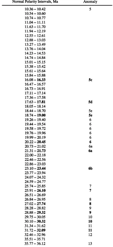
TABLE 1. Magnetic Reversal Time Scale Used in This Study Normal Polarity Intervals, Ma Anomaly

10.36- 10.42 5 !0.54 - !0.60 10.74- 10.77 11.04- 11.11 11.63- 11.70 11.94- 12.19 12.55- 12.61 12.88-13.03 13.27- 13.49 13.76- 14.04 !4.23 - !4.53 14.74- 14.84 15.01- 15.15 15.38- 15.42 15.61-15.64 15.84- 15.88 16.08 - 16.33 5c 16.47- 16.57 16.73- 16.91 17.11- 17.14 !7.36 - !7.58 17.63 - 17.81 5d 18.05- 18.14 18.44- 18.70 5e 18.74-19.00 5e !9.26 - !9.40 6 19.44- 19.54 6 19.58- 19.72 6 19.76- 19.96 6 19.99- 20.19 6 20.22- 20.45 6 20.73- 21.02 6a 21.31 - 21.73 6a 22.00 - 22.18 22.46- 22.56 22.86- 23.03 23. !0 - 23.44 6b 23.77- 23.94 24.07- 24.32 24.59- 24.77 25.74- 25.85 7 25.91 - 26.10 7 26.5 ! - 26.69 26.84- 26.95 8 27.02- 27.74 8 28.28- 28.82 9 28.88- 29.32 9 29.75 - 30.05 10 30.10- 30.32 10 31.34- 31.62 11 31.72- 32.09 11 32.46- 32.96 12 35.51 - 35.71 35.77- 36.12 13

Bold: picked anomalies.

last selected leads to a larger misfit [Patriat, 1987]. The second

method is an inverse method first described by Hellinger [1981], and refined by Chang [1987] and Royer and Chang [1991], who developed the software we used. The points at which isochrons are picked are grouped to define segments of either magnetic lineations or transform faults, paired before computation, and treated as arcs of great circles. The great circles and the rotation to fit them are determined by least squares. The misfit between the points and the great circles is used to compute the corresponding 95% confidence region, which represents the set of admissible poles and angles of

BRIAIS ET AL.: RECONSTRUCTIONS OF THE SOUTH CHINA SEA 6303

This Study LaBrecque (1977)

15 Ma - 20 Ma - 25 Ma - 30 Ma - 35 Ma - Patfiat (1987) s N symmetrical part Berggren et al. (•985) lO 11 5d 5e 6 6a 6b 6c 7 8 9 10 11 12

Fig 2. Comparison of magnetic reversal time scales. Normal polarity blocks are solid. Symmetric synthetic profiles calculated,

for scales of LaBrecque et al. [1977] and this study, assuming a 400-m-thick magnetized layer under a ridge oriented E-W at 15øN, 117øE since its creation.

rotations. The confidence region may be visualized as an ellipse in

the latitude-longitude plane. It becomes very large when the angle

of rotation is small. We used this method to visualize the

confidence regions of the poles of rotations. A finite pole of

rotation was obtained independently for each magnetic anomaly.

Stage poles, describing the rotation between two consecutive magnetic anomalies, were then computed to characterize, step by step, the evolution of the rate and direction of spreading.

Structural observations were used to separate the eastern, north- western and southwestern oceanic subbasins (Figure 1), and to re-

6304 BRIAIS ET AL.: RECONSTRUCTIONS OF THE SOUTH CHINA SEA

late the characteristics of the fabric of the oceanic crust in each basin

to our model of magnetic isochrons. The location of the relict

spreading axis corresponding to the last spreading episode was de-

duced from the bathymetry and the geometry of inward-facing nor-

mal faults observed on seismic profiles and Sea Beam swaths. In

the southwest subbasin, this relict axis is also marked by a promi-

nent free air gravity anomaly low [Taylor and Hayes, 1983; Pautot et al., 1986, 1990; Hayes et al., 1987]. Along the axial part of the eastern basin, the Scarborough seamount chain (Figure 1) probably lies on or close to the relict axis [Taylor and Hayes, 1983; Briais et

al., 1989]. The fabric of the 200-km-wide axial part of that basin is

characterized by a blocky basement, with normal faults striking

ENE to NE and fracture zones striking NW, covered by a sedimen-

tary layer about 0.5-s thick (two-way travel time) [Pautot et al.,

1986, 1990; Briais et al., 1989]. North and southeast of the in-

ferred relict spreading axis, the sediment thickness increases signifi-

cantly, to 1.5-2 s (two-way travel time) and the basement becomes

much smoother [Taylor and Hayes, 1983]. To the southwest, the

fabric is characterized by normal fault scarps striking more homo-

geneously NE and fracture zone scarps striking NW [Pautot et al.,

1986; Briais et al., 1989]. The northwestern subbasin is a deep,

thickly sedimented oceanic trough between the passive continental

margin of South China and the continental blocks of Macclesfield

Bank and Paracels Islands. To the east, this trough is continuous

with the deepest northern part of the eastern basin where Taylor and

Hayes [1980, 1983] identified magnetic anomalies 8 to 11

(Figure 1). The large and sometimes sharp changes observed both

in the seafloor fabric and in the sediment thickness, which suggest

that the characteristics of the spreading changed abruptly in time

during the opening of the basin, clearly represent first-order

features to be explained by any kinematic model derived from the

magnetic data.

Identification of Magnetic Anomalies

Estimation of the age and overall anomaly sequence in the eastern basin. The several attempts we made to fit the anomalies observed

on the longest magnetic profiles from the eastern subbasin with se-

quences of the geomagnetic time scale confirm the Oligocene-early Miocene age of the sequence of anomalies, with spreading rates of the order of 20-30 mm/yr, as first inferred by Taylor and Hayes

[1980, 1983] (Figures 3 and 4a). These ages postdate the rifting

estimated to have started in the Paleocene-Eocene along the northern and southern continental margins of the eastern South China Sea

[e.g., Holloway, 1982; Hinz and Schliiter, 1985; Fricaut, 1984; Ru

and Pigott, 1986; Suet al., 1989]. The heat flow measurements are also consistent with an early to mid-Tertiary age for the ocean floor

[Watanabe et al., 1977; Anderson, 1980; Taylor and Hayes, 1980,

1983]. The most typical sequence to be recognized in the basin is the 6b-6 anomaly sequence. It is especially prominent in the north-

eastern part of the basin (Figures 3 and 4). Nowhere else in the

basin, to the south or southwest, is it found with the same typical

shape (Figures 6 and 7). A priority in our interpretation of the

anomalies in the eastern basin was to respect the broad shape of

anomaly 6, which is characteristic in most oceanic basins [e.g.,

Patriat, 1987], as well as the large amplitude of anomaly 6b, which

is prominent on both sides of the ridge (Figures 3, 4a, 6 and 7). It

should be noted that the skewness is such that a given time in the

magnetic time scale corresponds, within the uncertainty in picking

of the anomalies, to a negative anomaly to the north of the profile,

and to a positive anomaly to the south of the profile (Figures 2, 4

and 7).

Old crust in the eastern basin. The oldest magnetic lineations that

could be identified are anomaly 11 in the north and 10 in the south

(respectively, 32 Ma and 30 Ma, Figures 3 and 4). Magnetic

anomalies in the southeast have a lower amplitude than in the north- east, and anomalies 8 to 10 are not observed near the southeastern

continental margin (Figures 3 and 4a). We discuss possible causes

for this asymmetry in the section concerning reconstructions.

In the eastern basin, there is a greater number of magnetic anomalies north than south of the Scarborough relict axis

(Figure 4a). This asymmetric distribution implies that the ridge

jumped to the south, as Taylor and Hayes [1983] first inferred.

Placing this jump just after anomaly 7 provides the best fitting syn- thetic magnetic profile (Figures 3 and 4a). The two conjugate

anomalies 7 are observed in the north. To the southeast, anomaly 7

is missing, and the large-amplitude anomalies 6b and 8 are juxta-

posed (Figures 3 and 4a). A fanning of the magnetic lineations,

spanning about 20 ø, is observed north of the ridge, revealing a

change in the overall trend of the spreading center, from N70øE for

anomaly 10, to N80øE for anomaly 8, and to E-W for the aban-

doned spreading center (Figure 3). This reorientation of the ridge system is accompanied by a reorganization of the ridge axis, which

we shall discuss in the section on the evolution of the spreading system.

Northwestern basin. Previous data were too scarce to identify

magnetic anomalies in the northwestern subbasin, although seismic

data suggested that it is underlain by oceanic crust. The new pro- files confirm this view and reveal symmetrically magnetized crust.

Because this oceanic trough is particularly narrow (•150 km), the correlation of observed profiles with a magnetic model is not unique

(Figure 5). Nevertheless, only three sequences, consisting of

anomalies 10-11, 13-15 or 21-22, provide an acceptable match to

the observed profiles. Of these three possibilities, the 10-11 se- quence is most consistent with structural and stratigraphic observa-

tions, because it allows continuous spreading over the whole north-

ern basin in the early Oligocene (Figures 3, 4a and 5).

Ridge jump at the time of anomaly 7 and correlative ridge reor-

ganization. To the east, the ridge jump after anomaly 7 is confirmed by morphological observations of its effect on the ridge system. Since the conjugate anomalies 7, which bound the abandoned ridge axis, are separated by the same distance all along

that ridge, we infer that the jump was simultaneous for all

segments. The eastern spreading segments, however, jumped

farther south than the western ones (Figures 3 and 4a). The age

difference at the boundary between the old and new crust is thus

greater east of 117øE than to the west, as reflected by the larger

topographic step observed between these crusts [Rea, 1978; Patriat,

1987] on seismic profiles (Figure 4b). The jump was accompanied

by a reorganization of the ridge axis, characterized by the demise of

the previous left-stepping geometry, and the formation of more

continuous, mostly right-stepping axial ridge segments as observed

on isochron 6b (Figure 3).

The best-fitting synthetic profile also suggests a change in half

spreading rate at the time of the jump, from 24 mm/yr (in the west) to 29 mm/yr (in the east) before the jump, to 19 mm/yr after that

jump (Figure 4a). We infer that the increase in the roughness of

the seafloor observed on the seismic lines is due to the decrease in spreading rate (Figure 4b). A similar increase in the local rough-

ness of the oceanic crust with decreasing spreading rate has been

observed along the Indian Ocean ridges, which display half

spreading rates varying from less than 10 mm/yr to 20 mm/yr and

30 mm/yr for the Southwest, Central and Southeast Indian Ridges,

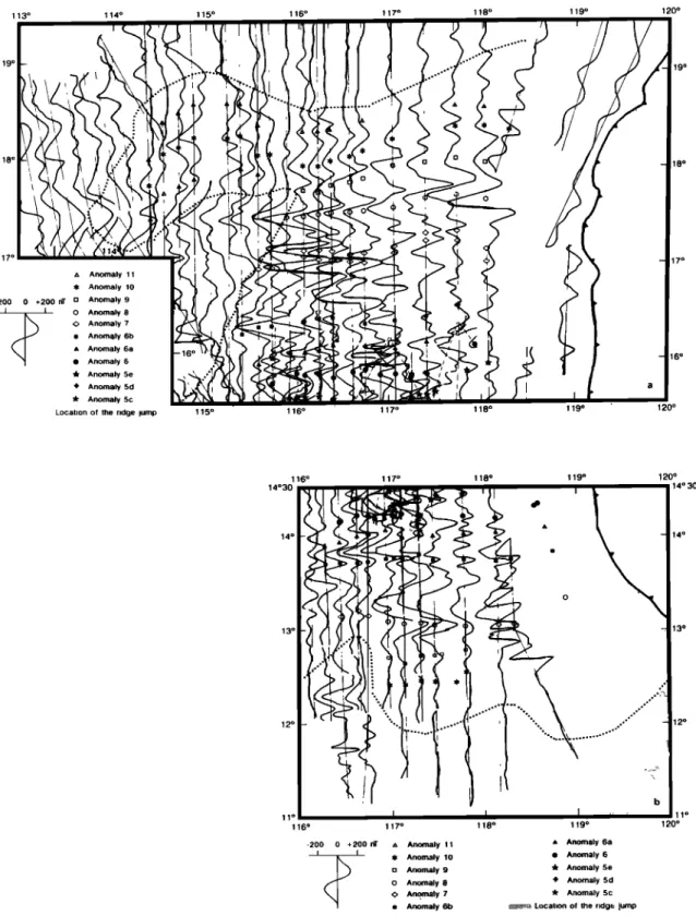
BRIAIS ET AL.: RECONSTRUCTIONS OF THE SOUTH CHINA SEA 6305 113 ø 114 ø 115 ø 116 ø 117 ø 118 ø 119 ø 120 ø 19 ø 19 o 18 ø 18 ø 17 ø /, Anomaly 11 • Anomaly 10 -200 0 +200 nT o Anomaly 9 O Anomaly 8 0 Anomaly 7 ß Anomaly 6b ß Anomaly 6a ß Anomaly 6 '• Anomaly 5e ,I, Anomaly 5d ß k Anomaly 5c

Locahon of the ridge lump 115 ø 116 ø 117 ø 118 ø 119 ø 120 ø 17 ø

16 ø

116 ø 117 ø 118 ø 119 ø ! 20 ø

14 ø 30' 14 ø 30'

11; 16 ø 117 ø 118 ø 119 ø

-2010

0 +2100

nT ,,, Anoma!y

1

1

ß Anomaly

6a

• •3

Anomaly

9

•'

Anomaly

5e

O Anomaly 7 '• Anomaly 5c

ß Anomaly 6b !•i•::•!•::•½•!:.!• Location of the ridge lump

14 ø

13 ø

12 ø

120 lø 1 o

Fig. 3. Magnetic profiles plotted along ship tracks in (a) northern and (b) southern parts of eastern basin. Frames A and B in

Figure

1. Barbed

line

is the

Manila

subduction

zone.

Dotted

line

is the

inferred

location

of continent-ocean

boundary.

Symbols

are

the

picks

of anomalies

identified

in this

study

(and

picks

of anomalies

on

Verna

profiles

from

Taylor

and

Hayes

[1983]).

Note

the

fanning

of anomalies

11

to 7, the

southwar

d ridge

jtimp

and

the

reorganization

of spreading

axis

at

time

of anomaly

7. Gray

dashed

line

is the

approximate

boundary

between

the

pieces

of crust

created

before

and

after

the

ridge

jump.

Short segments of isochron 7 are tentatively identified to the

northwest and to the southwest, along the continental margins

(Figures 3 and 4). The ridge therefore started to propagate towards

the southwest, between Macclesfield Bank and Reed Bank, at that time.

Axial eastern area. In the eastern area, after the ridge jump, the

magnetic isochrons appear to be more disrupted when approaching

the axis (Figures 3 and 6). Taylor and Hayes [1983] inferred that

disruption to result from the magnetization of the Scarborough

6306 BRIAIS ET AL.: RECONSTRUCTIONS OF THE SOUTH CHINA SEA

ß -•.-- N

29mmlyr I

19mmlyr

Synthetic

Profile

••

12 11 10 9 7 7 jump 6b 6a 6

I--I C]O OO

cDr--1

r---IOO

C3

on, onoOOill)OOo]•m•lDI

2oo]

C) OO DO C]C] [•)OO [] DO] 00000DOOOrr113CDD

24mm/yr 19mm/yr

19mm/yr

] 29mm/yr

• N

I•D•oDODODOOO • OO• • DO O•

no jump

19mm/yr 24mm/yr

Fig. 4. (a) Identification of magnetic anomalies in (left) northern and (right) southern parts of the eastern basin, showing the ridge

jump just after anomaly 7. Anomaly 7 is also tentatively identified on the southern parts of profiles NS11 to NS15. Data profiles

are projected on N180øE direction. Shown below the synthetic profiles are corresponding normal blocks in the time scale. (b)

Seismic profiles [from Taylor and Hayes, 1983] and location of ridge jump identified from magnetics, showing the correlation of

decreasing spreading rate with increasing basement roughness.

[e.g., Pautot et al., 1990]. This hypothesis, however, can only ac-

count for an abnormal magnetic signature close to the seamounts,

while the anomalies seem to be distorted farther off-axis as well (Figure 6a). The disruption is thus more likely attributed to the

geometry of the spreading axis itself, which includes numerous dis-

continuities [Briais et al., 1989].

For the sequence of anomalies 6b to 6 in the eastern subbasin

(Figure 7a), the eastern and western segments appear to have dis- tinct behaviors. East of 117øE, the best-fitting synthetic magnetic profile suggests that the magnetic sequences are rather symmetrical,

with a half spreading rate of about 18-20 mm/yr. West of 117øE,

the best fit is obtained with a model involving a small ridge jump

towards

the

south

at anomalies

6a-6

time,

and

a half

spreading

rate

of 19 mm/yr (Figure 7a). Another possible model involves

asymmetric spreading, with half spreading rates of 18-20 mm/yr

for the northern side of the ridge and =12 mm/yr for the southern

side. We have a slight preference for the former model because it

accounts best for the observation that anomalies 6 and 6a are repre- sented by a total of 3 picks in the southeast and only 2 in the south- west, and that anomaly 6 is particularly large to the northwest (near N15ø30, Ell6 ø , Figures 6 and 7). This change in the behavior of

the spreading center along strike probably explains why the 6b-6

sequence is more difficult to recognize south of the ridge than north of it, as initially noted by Taylor and Hayes [1980, 1983].

Southwestern basin. With the integration of the new profiles,

the magnetic data in the southwestern subbasin have become

especially dense, which frequently permits easy correlation of the

anomalies between the profiles. That such a correlation is easier

than in the central eastern basin suggests that the seafloor in the southwestern subbasin has been created along a spreading axis with

100krr

BRIAIS ET AL.: RECONSTRUCTIONS OF THE SOUTH CHINA SEA 6307

8

RIDGE

JUMP 6b

6 a

6

5 ©

Spreading

rate I

Spreading

rate

,• 2.5cm/yr -• 2cm/yr

Smooth basement rough basement

East

.., ..:.]!::. ....,, . .,. .• . N

i:

I

I

b

!.',

'

:'"

Fig. 4. (continued)

more simple geometry than that of the axis in the eastern basin. The

prominent free air gravity anomaly provides the location of the relict

spreading axis [Taylor and Hayes, 1983; Pautot et al., 1990]. As

in the northwest, the narrowness of the oceanic crust in this

subbasin, less than 150 km from the relict axis to the margin,

makes the match of observed anomalies with a synthetic model

nonunique. Four different sequences of anomalies, 6b-5c, 13-8,

19-13 and 26-21, of the reversal time scale provide synthetic profiles that resemble the observed magnetic profiles, with similar spreading rates, from 12.5 to 20mm/yr (FigureS).

Reconstruction of the geometry of the whole basin, however,

permits us to tentatively choose between these sequences.

Inspection of the shapes of the anomalies initially led us to

choose the sequence of anomalies 13 to 8, with spreading rates of 17 mm/yr in the north and about 11 mm/yr in the south. This in-

terpretation implied that spreading had ceased in the southwestern

subbasin 10 m.y. before it did in the eastern one, and therefore that

a major transcurrent zone existed near the boundary between the

eastern and southwestern subbasins. A model in which the ridge

was successively linked to eastward-jumping strike-slip faults could

have accounted for such a pattern of spreading (Figure 9 inset).

The uncontroversial identification of magnetic anomalies more re-

cent than anomaly 7 in the eastern basin, and the reconstruction of

its central part may be used to yield an image of the entire basin at

the time when spreading would have ceased in the southwest, in

that interpretation. This image (Figure 9) reveals a complex system

AXIS Preferred model 12 11

•

30-32

Ma

•

34-38

Ma

•

47-53

Ma

t'. '! '. '. '-'-'"'-•/'.

'. '. "./'. '-'- '•"" "'-:A

foø

oø

oø

oø

oø

,ø

oø

•x•

ø

oø

.ø

•ø

ß

oO

oø

oø

oø

oø

oø

oø

oø

oø

,,o::

::

::

::: .::

::'

18" 18 ø

' "' -" '" -' ti

113 ø 114 ø 115 ø 116 ø 117 ø

Fig. 5. (a) Identification of magnetic anomalies in the northwestern riff. Alternative synthetic profiles with an acceptable match with data are shown. Data profiles are projected on a N160øE direction. Gray dashed line is approximate location of the continent-ocean boundary. (b) Location of identified magnetic anomaly picks, showing NE-SW orientation of rift. Bathymetry in meters.

of ridge

segments,

in which

the

central

area

is occupied

both'by

an

isolated, abandoned rift to the north and an intervening continental block (Macclesfield Bank) to the south. Clearly, our data are insuf- ficient to argue for such complexity.

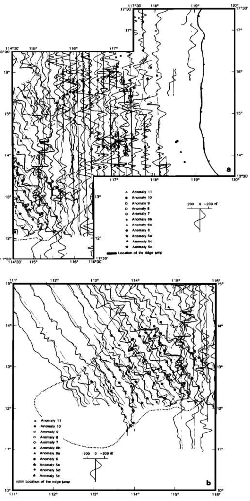
117o30 ' 118 ø 119 ø 120;7o30 , 17o30 ' 17 ø 17 ø 114o30 ' 11,5 ø 16o30 ' 116 ø 117 ø 16 ø 16 ø 15 ø 15 ø 14 ø 13 ø 12 ø 11 ø30' 114ø30 ' 115 ø 1 16 ø 117 ø 118 ø 119 ø ß • Anomaly 11 13ø • Anomaly 10 n Anomaly 9 o Anomaly 8 O Anomaly 7 ß Anomaly 6b & Anomaly 6a ß Anomaly 6 'A' Anomaly 5e 12 ø ,I. Anomaly 5d ß A. Anomaly 5c • Location of the ridge lump 11 ø30' 116030 ' -20[0 0 +2100 nT 14 ø 13030 ' 120 ø 111 ø 112 ø 113 ø 114 ø 115 ø 15 ø 116 ø 15 ø 14 ø 13 ø 13 ø 12 ø • Anomaly 11 • Anomaly 10 O Anomaly 9 o 11 ø _ ß '• Anomaly 5e ß Anomaly 5d W Anomaly 5c Locabon of the ridge lump

10 o J 111 ø 112 ø Anomaly 8 o. :" Anomaly 7 ."' Anomaly 6b ... '"' Anomaly 6a -200 0 +200 nT Anomaly 6 I i 12 ø 11 ø b 113 ø 1 14 ø 1 15 ø 116 ø

Fig. 6. Magnetic profiles plotted along ship tracks in axial area, (a) east and (b) southwest. Frames C and D in Figure 1. Dotted line is the inferred location of continent-ocean boundary. Barbed line is the Manila subduction zone. Symbols are the anomalies identified in this study. Note the stepwise southwestward propagation of oceanic spreading after anomaly 7.

BRIAIS ET AL.: RECONSTRUCTIONS OF THE SOUTH CHINA SEA 6309 o

I

Synthetic

6b

6a

6 5e

5d

5•

AXIS

200

3

50

I

100km

I

i •?•

,/

•

PN57-74

•

NS9

Fig. 7. Identification of magnetic anomalies in axial area of basin, (a) east, (b) intermediate, (c) southwest. Shown below the

synthetic profiles are corresponding normal blocks in time scale. All models are calculated for half spreading rate of 19 mm/yr.

Poor identification on profiles NS5-8 and NWl-13 reflects the complexity of the intermediate zone between Macclesfield and Reed Banks. The synthetic profiles at the bottom of Figures 7a and 7b include ridge jumps at the time of anomalies 6a-6 and 5e-Sd,

6310 BRIAIS ET AL.: RECONSTRUCTIONS OF THE SOUTH CHINA SEA

•

N

AXIS

--E

'•'•5'30'

•

NS8

NW1

••j•,..'"•,

NW

5

•

_

.

NS6

NW

7

6 6a

6b

200•

nT

o

I

NS5

•

NW9

•

NW11

0 50 100km

•_•

• v

••'•

•'ltl

N•15

Synthetic

profile

s I 5 •c

_mp

_6a

BRIAIS ET AL.' RECONSTRUCTIONS OF THE SOUTH CHINA SEA 6311 o I,

200-1

nTO-

//

/

•

NW

38

DC]D

rid

I 0 0 rl•DTITDOTD•••••

0 01

i• ODD

AXIS

Fig. 7. (continued)

This led us to abandon our initial match and to opt for a match

corresponding to the sequence of anomalies 6b to 5c (Figures 6

and 7). The main advantage of this match is that it yields a simple,

continuous geometry of magnetic isochrons across the whole central part of the basin. Moreover, fits of anomalies in the

southwestern part, using poles of rotation computed only from

anomalies identified in the eastern part, provide a positive test for

the choice of the 6b-5c sequence of reversals in the southwest.

That we could obtain a consistent set of Euler poles of rotation,

with reasonable confidence ellipses, for these anomalies is also an argument in favor of this choice. A problem that remains with this

alternative match, however, is that the amplitude and shape of

anomalies 6 to 6b in the southwest are different from those of the

same sequence in the east, where anomaly 6b is so easily

recognized (Figures 6 and 7). In fact, this new interpretation of the

southwest subbasin now hinges on the series of anomalies

observed on the northern side of profiles NW20-23, from anomaly

5c, close to the axis, to anomaly 6 or 6b, close to the margin

(Figures 6, 7b and c and 8).

The first identifiable anomalies along the margin are anomaly 6 in

the southwest (west of 115øE) and anomaly 6b in the intermediate

zone between the disrupted eastern and the southwesternmost axes

(from 115øE to 116øE) (Figures 6 and 7). This arrangement of the

6312 BRIAIS ET AL.: RECONSTRUCTIONS OF THE SOUTH CHINA SEA AXIS NW20 NW21 NW22 NW23 6c-5b 25-15.5my N • AXIS HSR 1.75cm/yr 13•.8 38-27.õmy 1.5cm/yr 18-13 45.5-'36my 26-20 6o'-46my 2.0cm/yr 1.25cm/yr

Fig. 8. Magnetic data profiles from (top) SW subbasin compared with (bottom) synthetic magnetic profiles corresponding to four different sequences of magnetic reversal time scale, showing that the interpretation is nonunique.

southwest in two major steps, first at the time of anomalies 6b-7, creating a new spreading axis in the intermediate zone, then at the time of anomaly 6, when the ridge reached its longest extent. The poorly developed shape of anomaly 6b in the southwest may be due to the fact that it represents the first anomaly along the margin, as

does anomaly 11 to the northeast.

The best fit with a synthetic magnetic profile is obtained with a

spreading rate of about 18 mm/yr on either sides of the axis.

Several profiles (NW20 to NW25, Figures 7b and 7c), however,

display prominent asymmetry. Synthetic profiles involving asym- metry in the spreading rates do not match the observations as well

as models invoking a ridge jump. Our preferred model thus in-

cludes one more small ridge jump along the segment defined by

these profiles at the time of anomaly 5d. As all other jumps inferred

from magnetic anomalies in the South China Sea, that jump was di-

rected toward the south.

Cessation of seafloor spreading. Because the axial part of the

eastern basin does not display any identifiable magnetic anomalies,

the last episode of spreading there may only be deduced from the

model for anomalies 6-5d, assuming a constant spreading rate after

anomaly 5d. This suggests a cessation of spreading near anomaly

5c (Figure 7a). The anomalies observed in the axial zone show

prominent variations of wavelength along strike (Figures 4 and 7),

which may be interpreted in terms of differential asymmetric

spreading related to the reorientation of spreading segments

[Menard andAtwater, 1968; Hey et al., 1988]. In the southwestern

part, the end of the spreading is observed just after anomaly 5c

BRIAIS ET AL.: RECONSTRUCTIONS OF THE SOUTH CHINA SEA 6313 18 ø 16 ø 14 ø 112 ø 114 ø 116 ø 118 ø

:.

:.y \::::: :)-/

_--

:(

\'::.://--'

_

....:

::

::

::

::

:: :-:

.:

.:

.:

.:

.:

.:

.:

.:

.:

.:

.:

.: .:

...:

Fig. 9. Computed reconstruction of the central eastern basin at time of the ridge jump (-An7) showing complexities implied if sequence of anomalies 8-13 is chosen. Inset: Sketches depicting model of evolution of spreading in South China Sea assuming spreading, and associated strike-slip faulting, ceased earlier in the southwest (1) than in the east, due to the activation of a new strike-slip fault to the east (2).

conclusion is thus that the cessation of spreading in the South China Sea was synchronous all along the ridge, just after anomaly 5c, at •15.5 Ma, although slight diachronism between the east and the southwest cannot be excluded. Note that this conclusion is a direct consequence of our preferred anomaly sequence match.

RECONSTRUCTION OF SEAFLOOR SPREADING IN THE SOL/TH CHINA SEA

The set of all the magnetic lineations deduced from the analysis

described above is presented in Figure 11, along with all the tec-

tonic features observed on Sea Beam swaths. The segmentation of

the isochrons derives from the fits of magnetic anomalies identified

on the profiles, resulting in the same shape of the isochrons on

either side of the ridge. By fitting these magnetic isochrons we cal- culated the Eulerian poles of rotation. We present here the results

of the fits and the reconstructions of the oceanic part of the basin,

without considering the surrounding continental areas. We discuss

the parameters of rotation calculated from these fits (Tables 2-4)

and the major steps in the evolution of the spreading ridge

(Figures 10-12). To assess the limit of the oceanic crust, we took

into account the gravity anomalies defined in the gravity profiles of

Taylor and Hayes [1983] and in the free air gravity anomaly map

published by B. Chen et al. [1987]. We also took into account the

magnetic profiles, especially along the northern and southwestern

limits of the basin. The oldest, southeasternmost part of the oceanic crust in the basin appears to be partly concealed under a recent com-

pressional thrust wedge and the thick sedimentation derived from it.

That interpretation is supported by seismic evidence [Taylor and

Hayes, 1983], and by the existence of a slice of Mid-Oligocene

oceanic crust inferred to have been part of the South China Sea

floor and obducted onto Mindoro Island in middle Miocene time

[Rangin et al., 1985].

Finite and Stage Poles of Rotation

Using both Patriat's [1987] and Hellinger's [1981] methods, we

adjusted the parameters of rotation to obtain a consistent set of stage poles, with no abrupt change in spreading direction and rate. The isochrons in a small ocean basin like the South China Sea are rela- tively short and close together, so that a simple best fit may lead to inconsistencies. To constrain the fit of anomalies older than anomaly 7 in the eastern basin, we thus used the additional obser-

vation that the anomalies abut the continental margin, west of

Macclesfield Bank to the north and of Reed Bank to the south

(Figure 11). The fit of magnetic anomalies younger than anomaly

7 is constrained by the elbow shape of the axis. The greatest uncer- tainty is in the central axial zone of the basin, due to the poor mag- netic data and large number of seamounts. Hence as an additional constraint to fit anomalies 5e to 5c in this zone, we tried to respect the orientation of the fault scarps observed on Sea Beam bathymet-

ric swaths (Figure 11). The only magnetic isochrons that are sig-

nificantly offset by fracture zones are anomalies 10, 6b and 5d

(Figures 3, 6 and 11). The fact that we could clearly identify most

of the segments of these anomalies on either side of the ridge pro-

vided a valuable constraint for the fit. Such a constraint could not

be used for other isochrons, however, because they were either not disrupted by fracture zones, as in the case of anomalies 9 or 8, or too disrupted by short-offset discontinuities, as for anomalies 6 to 5d in the east.

Because small ridge jumps occurred at the times of anomalies 6

and 5d (Figure 7), the corresponding reconstructions are less cer-

6314 BRIAIS ET AL.' RECONSTRUCTIONS OF THE SOUTH CHINA SEA

TABLE 2. Finite Rotation Parameters

Anomaly Age, Ma Latitude, deg Longitude, deg Angle, deg Patriat's [1987] Method 5c 16.56 -3.0 93.6 0.7 5d 17.81 5.0 105.5 3.7 5e 19.00 -1.4 88.7 2.4 6 20.45 0.1 83.3 2.8 6a 21.73 0.1 81.3 3.5 6b 23.44 -1.1 75.9 3.9 jump 25.91 7.0 87.8 7.5 8 27.74 9.3 91.2 10.3 9 29.32 8.2 87.4 10.3 10 30.32 7.9 85.7 10.8 Hellinger's [1981] Method 5d 17.81 5.70 105.01 3.79 5e 19.00 0.09 92.26 2.72 6 20.45 -4.52 74.37 2.32 6a 21.73 -0.50 78.60 3.26 6b 23.44 0.02 84.61 4.78 8 27.74 9.73 92.95 10.98 9 29.32 11.12 94.02 13.29 10 30.32 8.27 86.79 11.20

Positive latitudes and longitudes are northern and eastern hemisphere, respectively. TABLE 3. Stage Poles and Angles of Rotation

Anomalies Age End, Ma Time Span, m.y. Latitude, deg Longitude, deg Angle, deg Patriat's [1987] Method End- 5c 15.64 0.69 -3.0 93.6 0.7 5c- 5d 16.33 1.48 6.7 108.2 3.0 5d-5e 17.81 1.19 -12.9 -47.8 1.6 5e - 6 19.00 1.45 7.3 58.0 0.5 6-6a 20.45 1.28 0.4 72.9 0.7 6a- 6b 21.73 1.71 -7.2 39.1 0.6 6b - jump 23.44 2.47 14.2 101.0 3.4 jump - 8 25.91 1.83 14.3 101.0 3.3 8- 9 27.74 1.58 -10.7 2.7 0.7 9- 10 29.32 1.00 4.4 55.8 0.6 10- 11 30.32 1.77 10.9 84.9 1.4 Hellinger's [1981] Method End - 5d 15.64 2.17 5.7 105.0 3.79 5d- 5e 17.81 1.19 -15.4 -46.6 1.33 5e - 6 19.00 1.45 -11.0 -33.1 0.90 6 - 6a 20.45 1.28 8.8 89.0 0.98 6a-6b 21.73 1.71 0.6 97.3 1.57 6b - 8 23.44 4.30 16.2 100.1 6.41 8- 9 27.74 1.58 17.0 100.0 2.33 9- 10 29.32 1.00 -17.3 -51.2 2.65 10- 11 30.32 1.77 10.1 84.1 1.36

Poles and angles computed for southern flank of the ridge from finite rotations in Table 2. Positive latitudes and longitudes are northern and eastern hemisphere, respectively.

however, they may be considered to reflect a mere asymmetry in spreading. We therefore include the results of the fits of anomalies 5d and 6, noting that the uncertainty for them is greater. The pa- rameters of rotation at the time of the large jump after anomaly 7 are interpolated from those corresponding to anomalies 8 and 6b.

Since anomaly 11 is only tentatively identified on both sides of the narrow rift in the northwest, we calculated the pole of rotation corresponding to the stage between anomaly 11 and anomaly 10,

which forms the axis of that rift.

Uncertainties on the rotation parameters were computed using

Hellinger's [1981] method. The results of the computations were

unstable and varied as a function of the data points considered. The

95% confidence ellipses are shown in Figure 12a. For anomaly

5c, no acceptable confidence ellipse was obtained, although a good fit was reached using Patriat's [1987] method. The confidence el-

lipses for anomalies 11 and 9 are very large. For anomalies 11 and 5c, the conjugate picks are very close to one another, implying a very small rotation angle and therefore a greater uncertainty. For anomaly 9, the great uncertainty is probably related to the shape of the isochron, which consists of short segments without significant

offset. For other anomalies, the confidence ellipses are smaller

(Figure 12a) but are always elongated in a direction parallel to the

isochrons, which reflects the absence of large-offset transform

faults, and the relatively short length of all the isochrons.

The finite poles of rotation are all located to the SW of the basin,

the poles corresponding to anomalies 10 to 8 being closer to the

basin than the poles corresponding to the younger phases of

seafloor spreading (Figure 12a). The stage poles of rotation are

much more scattered, but roughly aligned on a great circle. Using