HAL Id: insu-03011247
https://hal-insu.archives-ouvertes.fr/insu-03011247
Submitted on 18 Nov 2020HAL is a multi-disciplinary open access archive for the deposit and dissemination of sci-entific research documents, whether they are pub-lished or not. The documents may come from
L’archive ouverte pluridisciplinaire HAL, est destinée au dépôt et à la diffusion de documents scientifiques de niveau recherche, publiés ou non, émanant des établissements d’enseignement et de
Linking thermochronological data to transient
geodynamic regimes; new insights from kinematic
modeling and Monte Carlo sampling of thermal
boundary conditions
Nassif Sanchez, Kerry Gallagher, Miguel Ezpeleta, Gilda Collo, Federico
Davila, Andres Mora
To cite this version:
Nassif Sanchez, Kerry Gallagher, Miguel Ezpeleta, Gilda Collo, Federico Davila, et al.. Linking thermochronological data to transient geodynamic regimes; new insights from kinematic modeling and Monte Carlo sampling of thermal boundary conditions. Journal of South American Earth Sciences, Elsevier, 2021, 105, pp.103018. �10.1016/j.jsames.2020.103018�. �insu-03011247�
Journal Pre-proof
Linking thermochronological data to transient geodynamic regimes; new insights from kinematic modeling and Monte Carlo sampling of thermal boundary conditions Sanchez Nassif Francisco, Gallagher Kerry, Ezpeleta Miguel, Collo Gilda, Davila Federico, Mora Andres
PII: S0895-9811(20)30561-7
DOI: https://doi.org/10.1016/j.jsames.2020.103018
Reference: SAMES 103018
To appear in: Journal of South American Earth Sciences
Received Date: 29 May 2020 Revised Date: 14 October 2020 Accepted Date: 6 November 2020
Please cite this article as: Francisco, S.N., Kerry, G., Miguel, E., Gilda, C., Federico, D., Andres, M., Linking thermochronological data to transient geodynamic regimes; new insights from kinematic modeling and Monte Carlo sampling of thermal boundary conditions, Journal of South American Earth
Sciences (2020), doi: https://doi.org/10.1016/j.jsames.2020.103018.
This is a PDF file of an article that has undergone enhancements after acceptance, such as the addition of a cover page and metadata, and formatting for readability, but it is not yet the definitive version of record. This version will undergo additional copyediting, typesetting and review before it is published in its final form, but we are providing this version to give early visibility of the article. Please note that, during the production process, errors may be discovered which could affect the content, and all legal disclaimers that apply to the journal pertain.
Conflict of interest
The authors whose names are listed immediately below certify that they have NO affiliations with or involvement in any organization or entity with any financial interest (such as honoraria; educational grants; participation in speakers’ bureaus, membership, employment, consultancies, stock ownership, or other equity interest; and expert testimony or patent-licensing arrangements), or non-financial interest (such as personal or professional relationships, affiliations, knowledge or beliefs) in the subject matter or materials discussed in this manuscript.
Author names:
Francisco Sanchez Nassif Kerry Gallagher Miguel Ezpeleta Gilda Collo Federico Dávila Andres Mora.
Journal Pre-proof
Linking thermochronological data to transient geodynamic regimes; new insights 1
from kinematic modeling and Monte Carlo sampling of thermal boundary conditions 2
Authors: Sanchez Nassif, Francisco1; Gallagher, Kerry2; Ezpeleta, Miguel1; Collo, Gilda1,
3
Davila, Federico1, Mora, Andres3
4
1. Centro de Investigaciones en Ciencias de la Tierra (CICTERRA). Av Velez
5
Sarsfield 1699, Cordoba, Cordoba, Argentina.
6
2. Geosciences/OSUR, University of Rennes, Campus de Beaulieu, Rennes, 35042,
7
France
8
3. Ecopetrol, Praia de Botafogo, Brazil
9
Abstract 10
It is common practice to assume values for basal heat flow or basal temperatures as a
11
lower boundary condition for thermo-kinematic models of crustal tectonics. Here, we infer
12
spatial and temporal variations of the paleo-basal temperature from integrated modelling of
13
thermochronological ages, to relate the inferred variations to the geodynamic setting. To
14
this end, we consider the Argentine Precordillera as a natural laboratory, given that its
15
kinematic evolution is relatively well constrained and therefore, the focus can be placed on
16
the variations of its basal thermal state. By means of a simple Monte Carlo sampling
17
approach with thermochronological data as constraints, we infer the paleo-basal
18
temperature history. This is compared to estimates posed by models existing in the
19
literature concerning flat-slab subduction. Our results imply that, given the kinematic
20
models used to date in the area, extremely low temperature gradients (< 15°C/km) are
21
required to adequately predict the observed thermochronological ages. Substantial cooling
22
of the lithosphere around 10 Ma is also required in order to fit measured values. This
23
agrees with previous thermal simulations carried out in the region. Furthermore, major
24
controls of the thermal architecture on the Argentine Precordillera are implied, thus
25
reigniting the debate on thermal driving mechanisms in the evolution of mountainous
26
settings and their relationship with deeper processes within the Earth, such as on the
27
effects of the flat-slab subduction.
28 29 30
Introduction 31
Thermochronological data have been extensively used as constraints for models of the
32
thermal evolution of the lithosphere (see Reiners and Ehlers, 2005; Guillaume et al.,
33
2013., Dávila and Carter, 2013; Fosdick et al., 2015; and also England and Molnar, 1990;
34
Ring et al., 1999; for a review of cooling processes). In that sense, the growing use of
35
thermochronological data has propelled major advances in kinematic thermochronological
36
modeling in the last two decades (Braun et al., 2012; Almendral et al., 2015, among
37
others). Moreover, inverse thermochronologic modeling carried out under the assumption
38
of constant lower boundary conditions (such as basal temperature or heat flow) has
39
rendered valuable information on heat transfer in settings where the geodynamic evolution
40
is relatively well understood (Braun, 2003; Fillon and van der Beek, 2012; Coutand et al,
41
2014; Olivetti at al., 2017). In general, the lower boundary conditions are rarely treated as
42
variable (spatially and/or temporally) parameters (although see Schildgen et al., 2009 for
43
an example of transient lower thermal boundary conditions). Furthermore, no studies have
44
focused on inferring transient boundary conditions from thermochronological
45
measurements. Not taking geodynamic variability into account in regions where major
46
changes have clearly occurred (e.g. modification of the subduction angle; see for example
47
Dávila et al., 2018), can lead to equivocal results and conflicting interpretations. These
48
concerns are corroborated by studies demonstrating the thermal evolution of the
49
continental lithosphere is dependent on the evolving geodynamic scenario (Vitorello and
50
Pollack, 1980; Sachse et al., 2016; Ávila and Dávila, 2020). Thus, the relationship between
51
transient geodynamics and thermochronological modeling of the upper crust calls for
52
special attention.
53
To understand the implications of unsteady subduction and, as would be likely, an
54
unsteady or transient lower boundary condition for the overlying lithosphere, we consider
55
the well-known Argentine Precordillera (AP) as a preliminary case study. Structural
56
reconstructions in the Jachal area (near Jachal city, see Fig. 1; Jordan et al., 1993;
57
Allmendinger and Judge, 2014; Nassif et al., 2019) have been complemented with
58
thermochronological data (Levina et al., 2014; Fosdick et al., 2015; Val et al., 2016; and
59
new data from this work) and estimations of erosion rates (Fosdick et al; 2015; Val et al.,
60
2016; Nassif et al., 2019). These multiple constraints make the Argentine Precordillera of
61
Jachal an ideal test case to assess the potential of extracting novel geodynamic
62
information from measured thermochronological ages. Furthermore, the present work
63
seeks to build on previous findings exploring the influence of basal temperatures on
64
thermochronological data (see for instance Shildgen et al., 2009), and also to cast new
65
light on heating mechanisms. As has been previously suggested (Ehlers, 2005; Dávila and
66
Carter, 2013; Nassif et al., 2020, in press), physical phenomena other than burial and
67
denudation processes may play a significant role regarding rates and durations of heating
68
and cooling. Hence, we take advantage of the state-of-the-art knowledge of the Argentine
69
Precordillera to pose questions not directly concerning exhumation and/or erosion. In
70
particular, can we constrain variations of paleo-basal temperatures with kinematic and
71
thermochronological data? What implications may such estimates have on our
72
interpretations and thermochronologically driven conclusions? The present effort
73
addresses those questions by means of Monte Carlo sampling to infer basal temperature
74
values over time. We apply an easy-to-implement statistical framework to compare model
75
predictions with existing and new thermochronological data. These data are
76
complemented with diagenetic indicators (% Illite to Smectite; see Środoń et al., 1986),
77
the combination of which lets us set bounds on the lower thermal boundary condition, i.e.
78
basal temperature over time. The model results are compared to proposed thermal states
79
in the study region (Gutscher et al., 2000) which are of particular importance given the
80
uncommon nearly-flat subduction angle in the region. We propose that the stochastic
81
sampling approach described here may be suitable for other geological scenarios where
82
inversion of thermochronological data can aid reducing uncertainties of first-order variables
83
present in thermal simulations.
84 85
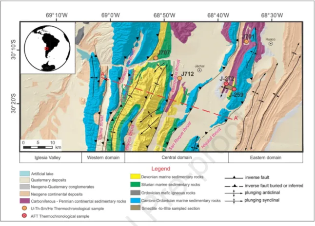
Geological setting 86
The Argentine Precordillera (AP) is an intraplate fold-and-thrust belt located at the
87
southern end of the Central Andes foreland. It is composed of N-S trending mountains that
88
record a prolonged Paleozoic to Cenozoic tectonic history, suggested being controlled by
89
subduction processes and the accretion of exotic terranes (Ramos et al, 1986; 2004).
90
Major Andean deformation and uplift in this region have been related to the ongoing flat
91
subduction of the Nazca plate beneath the South American lithosphere (Isacks et al.,
92
1982; Jordan et al., 1983a-b; Kay and Abbruzzi, 1996; Dávila et al., 2018).
93
The present-day landscape in the AP shows meridional and sub-parallel thrust sheets
94
separated by seven major thrust faults, named from west to east: Tranca, Caracol W,
95
Caracol E, Blanco, Blanquitos, San Roque, and Niquivil (Fig. 1; Allmendinger and Judge,
96
2014). Such structures, suggested to be associated with a deep decollement (~ 16 km),
97
are responsible for the complex scenario outcropping in Jachal section (see Fig 1). Studies
98
of the chronology of motion of the thrustbelt have elucidated its kinematics (Allmendinger
99
and Judge, 2014; Jordan et al., 1993), and have been complemented by recent efforts to
100
estimate Tertiary erosion and deposition (Fosdick et al., 2015; Val et al., 2019; Nassif et
101
al., 2019). Taken together, the structural and thermochronological endeavours in the area
102
have successfully constrained the spatial evolution of the region, but kinematic models
103
relating such deformation to the thermal evolution of the belt remain to be developed.
104
Given that the AP constitutes an exploratory frontier (Pérez et al., 2011), insights into the
105
thermal history experienced by potential source-rocks within the Cambro-Ordovician
106
limestone sequence. (Pérez et al., 2011; see Fig. 1 for reference), are of importance to
107
both researchers and industry.
108
Regarding its thermal state, the AP has been linked to refrigerated thermal regimes, as it
109
sits over the Chilean-Pampean flat slab segment (see Collo et al., 2018). Shifting of the
110
asthenospheric wedge caused by slab flattening is suggested to produce thermal cooling
111
of the upper crust (Gutscher et al., 2000; English et al. 2003; Álvarez et al. 2014), with
112
evidence of the 'cold state' provided in the Vinchina Basin. Here extremely low heat flow
113
values (< 30 mW/m2) were proposed to explain thermal calibration data (Collo et al., 2011;
114
2015). Such low heat flow values may have varied with the slab geometry, which has also
115
been constrained in the study region. Several authors (Gutscher et al. 2000; Jordan et al.,
116
2001; Ramos and Folguera, 2009; among others) have postulated the beginning of the
117
flattening episode at ~15-18 Ma, with the slab becoming sub-horizontal at ~7-6 Ma
118
(Gutscher et al. 2000; Kay and Mpodozis, 2002). Taking into account the already
119
understood spatial deformation at Jachal (see Fig. 1, above), the available data and
120
interpretations make this region of the Pampean flat slab an ideal scenario to explore the
121
relationship between a) the record of crustal cooling and exhumation, and b) the combined
122
effects of thin-skinned deformation and changes in subduction geometry at the lithospheric
123
scale.
124 125
126 127
Methodology 128
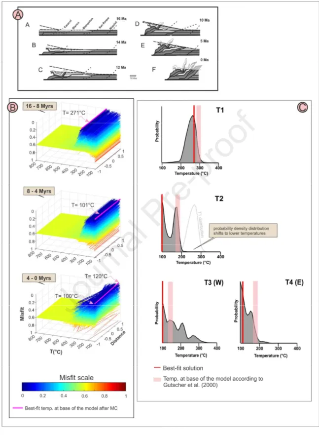
a) Inversion of time-dependent boundary conditions from thermochronological and 129
kinematics data 130
Using the documented deformational sequence for the AP (see Jordan et al., 1993;
131
Allmendinger and Judge, 2014; Nassif et al.; 2019, and references therein) as a geological
132
reference framework, we used Fetkin (Finite element kinematics; see Almendral et al.,
133
2015) to predict thermochronological ages along the thrustbelt. Fetkin is a 2D
thermo-134
kinematic code which takes as input a series of structural sections to forward-model
low-135
temperature thermochronological ages at user-specified locations by solving the heat
136 equation, given as 137 ( ) ( ) T C T q C T H t
ρ
λ
ρ
∂ = ∇⋅ ∇ − ⋅∇ + ∂ 138where T is temperature, t is time, is the thermal conductivity, ρ and C are the density
139
and specific heat capacity, respectively; and q is the rock velocity, determined by the
140
tectonic history of the setting. Rock velocities are obtained directly in Fetkin by tracking the
141
position of material particles throughout the simulation of the structural evolution. H
142
represents heat sources and sinks, which for simplicity, were not included in the models
143
considered here. Moreover, to solve the 2D form of the heat transfer equation, four
144
boundary conditions; namely B1 (lower), B2 (upper), B3 (right boundary) and B4 (left 145
boundary) are required. In this work, the lower boundary condition, B4, was allowed to vary 146
over time to better represent the geodynamic evolution of the system. The numerical
147
model starts from an equilibrated thermal steady-state, thereafter solving the heat equation
148
considering thrusting kinematics and boundary enforcements.
149
Our thermo-kinematic model for the Jachal AP (see Fig. 1 for location) started at 16 Myrs,
150
when movement along the westernmost thrust, Tranca (see Fig. 1), was triggered (Jordan
151
et al., 1993; Allmendinger and Judge, 2014). Thermo-kinematic calculations were carried
152
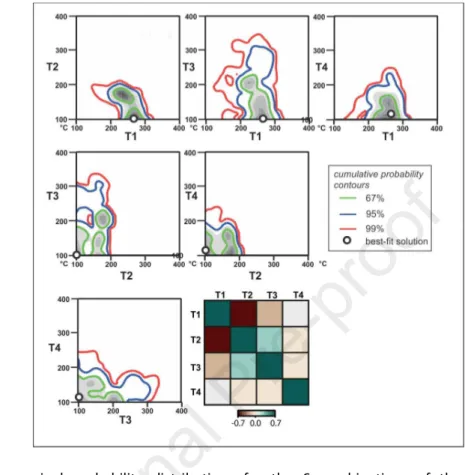
out to the present day, with the final model form being equivalent to the outcropping
153
structural configuration today (see Allmendinger and Judge, 2014; Nassif et al., 2019). For
154
λ
the thermal model calibration, we incorporated 2 sets of unpublished fission track data
155
(processed by Late Andes laboratory, Argentina, see Table 1). Sample J272, belonging to
156
Permian strata within the San Roque nappe (see Fig. 1 for location in the thrustbelt),
157
yielded a central AFT age of 152.3±12.9 Ma. Track lengths measurements were also
158
carried out in this sample, resulting in a unimodal distribution with a mean track length
159
(MTL) of 10.17 ± 1.68 μm (see Table 1 and also Supplementary Material, S1). In the
160
easternmost nappe, Niquivil, analysis in a Silurian sandstone yielded a central AFT age of
161
10.9 ± 2.1Ma, but no track lengths were observed in this sample. It is highlighted that the
162
two central ages obtained (ages for samples J259 and J272) were concordant (passed the
163
chi-squared test, see Supplementary Material 2) and are also considerably younger than
164
their stratigraphic ages. Moreover, no appreciable relationship between the single grain
165
ages and the kinetic parameter considered, Dpar (measured on each grain) was seen in
166
any sample (see Supplementary Material). These ages are therefore considered to reflect
167
primarily the post-depositional thermal history and are interpreted in terms of the samples'
168
cooling to the surface.
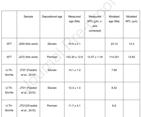
169 170 Sample X Y Z (m) Geologic unit Ns Ni Nd Rho-d (1/cm2 ) grains Dpar (μm) MTL(μm) U (ppm) Central
ages (Ma) Disp. P(X
2 ) J272 68.64° W 30.30° S 1125 Fm Panacan 777 519 10000 6.48E+05 15 1.46 10.16 37.52 152.3+-12.9 0.06 34.98 J259 68.62° W 30.31°
S 1195 Fm Los Espejos 33 314 10000 6.48E+05 21 1.36 no
lengths 17.21 10.9+-2.1 0.13 46.51 Table 1. AFT data from this work
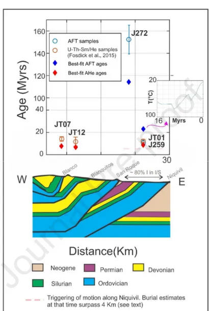
171 172
In addition to the new AFT measurements, data from 3 U-Th/He samples are available
173
from the literature (Fosdick et al., 2015; see Fig. 4, results) and these were also
174
incorporated as constraints. Finally, in order to complement the inferences based on the
175
thermochronological data, diagenetic indicators in clays (Smectite to Illite, I/S%) were also
176
measured along the easternmost nappe, Niquivil; following standard procedures for clay
177
treatment at the clay laboratory at Universidad Nacional de Córdoba (see Środoń et al.,
178
1986; an references therein).
179
Regarding the 2D heat transfer and thermochronological age simulations, the model
180
considers: a) a mesh resolution of 2500 nodes covering the modeled thrust belt ; b) a
181
timestep of 1 Myr; c) kinetics for AFT and U-Th-Sm/He from Ketcham et al. (2007) and
182
Wolf et al. (1998), respectively; d) an inherited age of 152 Myrs for the apatites in the study
183
region before Andean deformation took place. The last assumption is based on AFT
184
detrital results that registered such age (152.3 ± 16 Ma; see sample HC07 from Fosdick et
185
al., 2015) in grains from the foreland basin, Huaco (see Fig. 1 for location). Likewise,
186
results (this work) from AFT measurements in an eastern nappe of the thrust belt (San
187
Roque nappe; 152.3 ± 12.9 Ma; see also Supplementary Material); point also to a
188
Mesozoic inherited age of apatite grains before Andean deformation started in the AP (16
189
Ma). The program assumes the same inherited age for all thermochronological systems,
190
which poses no major problems in modeling exercises as long as thermal resetting in
U-191
Th-Sm/He samples is guaranteed (as occurs in this work; see results). Radiation damage
192
effects on He retentivity were not incorporated into the modelling (see also Limitations and
193
further insights)
194
The depth scale of the model, i.e. the depth to the lower thermal boundary condition, was
195
defined to be 20 km. In accordance with lithological characterizations in the area stating
196
that the thrustbelt is mostly composed by siliciclastic sediments (see Allmendinger and
197
Judge, 2014), we assigned a thermal conductivity of 2.5 W/m*K, a density of 2500 Kg/m3
198
and specific heat of 1000 J/kg*K (see Hantschel and Kauereauf, 2009; for value
199
references) across the whole model. Given the limited amount of calibration data, a more
200
complex set of thermophysical parameters or the inclusion of heat production, was not
201
justified for this preliminary study. The top boundary condition at mean sea level was set to
202
23 °C, after climate characterizations in the region (arid to semi-arid for the studied time
203
interval; see Walcek and Hoke, 2012).
204
As the aim of this work is to infer the lower thermal boundary condition
205
(temperature at 20 km), values for this parameter were allowed to vary in the range
100-206
800°C, corresponding to very low (5 °C/km) to high (40°C/km) thermal gradients (see
207
Hantschel and Kauereauf, 2009). These are broadly equivalent to a range in heat flow of
208
10 to 100 mWm-2. To allow for some time dependence, and following thermal numerical
209
models involving slab-flattening processes (Gutscher et al., 2000), we parameterized the
210
basal temperature history in 3 stages, in a step-function manner, with a constant but
211
unknown value in each stage. The time intervals considered for each stage were 1) 16-8
212
Ma, 2) 8-4 Ma and 3) 4 Ma to present (see Fig. 2). The time interval of the first stage was
213
selected to be relatively wide as that the slab-flattening process started around 20 Ma (Kay
214
and Mpdozis, 2002), and that its associated thermal effects would not have been
215
perceived before 10 Ma in the upper crust, equivalent to the depth scale of our model (see
216
Gutscher et al., 2000; Jaupart and Mareschal, 2010). Using simple Monte Carlo (MC)
217
sampling we select candidates for the basal temperatures in each time interval from the
218
temperature range defined earlier. To avoid drawing non-physical candidates (for example,
219
“scissor-like” ones implying rapid and large oscillations in the basal temperature), our
220
Monte Carlo sampling proceeded as follows: First, we drew a value from a uniform
221
distribution between 100°C (T min) and 800 °C (T max), corresponding to the first time
222
interval (16 to 8 Ma). Then, we drew a second value (part 2) from a uniform distribution
223
centered on the candidate value in the first time interval and extending 200°C on either
224
side. This large range (400°C) was set to ensure that a wide set of physically plausible
225
possibilities could be tested. The same prior lower and upper limits set (Tmin = 100°C, Tmax 226
= 800°C) as for the first part were also enforced in this instance, so samples were modified
227
accordingly when necessary (for example when values from the first draw corresponded to
228
temperatures near a limit). The basal temperatures for the first and second stages (see
229
Fig. 2) were constant in space, consistent with subduction numerical models that suggest
230
no major lateral variation in the relatively short spatial scale defined by the AP, at the
231
depth scale concerned by this work (see 2D predictions in Gutscher et al., 2000; Gutscher
232
and Peacock, 2003; Manea and Manea, 2011; and also 3D models in Ji et al, 2017; see
233
also Fig. 2). Finally, a candidate model was drawn for the final stage (part 3; 4 Ma to
234
present; Fig 2), using constrained sampling conditional on the value for the second stage,
235
as described previously. For this final stage, we also allowed for spatial variation for the
236
basal temperature (see Fig. 2) as flat-slab Andean thermal models predict an appreciable
237
gradient in the lateral direction (west-east) for this time interval (4 Ma to present; see
238
Gutscher et al., 2000). Hence, a candidate model for this part (3) consisted of two values,
239
both drawn from the same distribution (a uniform centered on the value for previous stage;
240
2). 10000 iterations of the process above described were performed, and the proposed
241
lower boundary condition temperature history were then entered into Fetkin to run a
242
thermal simulation for each iteration. As the final stage of a candidate model consisted of
243
two values (at the lateral boundaries), the values were interpolated linearly in space in the
244
Fetkin environment. A Python program to parallelize thermal modeling calculations carried
245
out by the Fetkin algorithm was deployed. To measure the agreement of predictions from
246
the thermal model with the observed data, we adopted the following misfit expression ( )
247
ϕ
248
where N the number of data sets and M the samples in each data set, the modeled
249
age for a particular set of parameters and the sampled value (measured age).
250
refers to the data uncertainty. Following Valla et al. (2010), we adopted an uncertainty of
251
0.5 Myrs to equally weight all data in terms of the difference between the observed and
252
predicted ages.
253 254
b) Additional views from classical inverse thermal history modelling 255
To complement insights derived from the 2D thermochronological simulations, we used
256
inverse thermal history modeling for samples J259 and J272, using the software HeFTy
257
(see Ketcham, 2005). To account for the depositional history of each sample, as well as
258
episodes of heating (potential resetting) before the period concerned by this work (16 Ma
259
to present), the inverse modeling exercises were set considering the following constraints:
260 Sample Time (Ma) Temp. range (°C) Rationale 400-280 >170 simulate provenance 300-280 0-30 sediment accumulation J272 260-80 60-140 burial heating 60-23 20-45
Paleozoic rocks should have been close to the surface anytime in the Cenozoic, as implied by the Neogene/Permian
unconformity in the maps
23-0 60-100 burial and heating of Paleozoic rocks as Andean-related
subsidence took place
500-440 >170 simulate provenance 440-420 0-30 sediment accumulation 300-90 60-140 burial heating
J259
60-23 20-45
Paleozoic rocks should have been close to the surface
(but deeper than sample J259, and therefore hotter)
anytime in the Cenozoic, as implied by the Neogene/Permian
unconformity in the maps
23-0 60-100 burial and heating of Paleozoic rocks as Andean-related
subsidence took place
261 2 ,mod , 1 1 (i i ) N M j j sam i i j j
α
α
ϕ
σ
= = − =∑ ∑
,mod jα
, j samα
i j σJournal Pre-proof
Table 2. Constraints considered in classical inverse thermal modeling.
262 263
Results and discussion 264
a) Misfit distribution 265
Results from the MC inversion are shown in Fig. 2. Fig. 2A shows the AP kinematics used
266
after Nassif et al (2019), which considered an in-sequence thrustbelt deformation starting
267
at 16 Ma. Fig. 2B displays a “noodle plot” of thermal candidates for each of the 3 periods
268
considered (16 Myrs to 8 Myrs, 8 Myrs to 4 Myrs, 4 Myrs to 0 Myrs), and their respective
269
misfit values. Misfits were normalized for this figure to a 0-1 scale, with 0 representing the
270
lowest misfit observed (best agreement between model predictions and data) and 1 the
271
highest (worst agreement between model predictions and data). We note that a
272
normalized misfit value of 0 does not represent a perfect agreement between data and
273
predictions. The distance along the AP axis is also shown rescaled (-1 to 1 representing
274
west to east; see Fig. 2). Finally, Fig. 2C shows 1D marginal distributions obtained via
275
Neighborhood Algorithm Bayes (see Sambridge, 1999), along with deterministic
276
temperature estimates at the base of the model (20 km) after the flat slab subduction
277
model of Gutscher et al (2000). Best-fit temperature candidates are also shown in Fig. 2C
278
for clarity (see red lines).
279
We remark that the conditional dependence (or correlation) between parameters from
280
each of the 3 periods plays a major role regarding the misfit values. For example,
281
normalized misfit values for T = 200°C in the first stage (16 Myrs to 8 Myrs; see Fig. 2B),
282
vary between 0.7 and 0.1, depending on the values of the other 3 parameters. Some
283
combinations of this candidate (T=200°C) with candidates from the other two stages
284
yielded better misfits than others, demonstrating a conditional dependence or trade-off
285
among values drawn for each of the 3 periods. Overall, however, basal temperatures in
286
the range between 400°C to 800°C represent poor models (high normalized misfit, 0.6 or
287
higher; see Fig. 2) for all of the 3 stages considered, regardless of how they were
288
combined.
289
Lower values of misfit for the first stage (16 Myrs to 8 Myrs) are obtained when candidates
290
are in the 300°C-100°C range (with some conditional dependence on the other two
291
periods, as discussed above). Misfit values are lower when candidates are around 200°C
292
to 100°C in the second stage (8 Myrs to 4 Myrs) , implying that basal temperatures (at 20
293
km depth) in the AP for this time interval may have decreased. This statement also holds
294
true for the third stage (4 Myrs to present). However, since a lateral variation of
295
temperature was allowed for this time interval of the simulations, the results appear more
296
dispersed across the temperature axis relative to the second phase. Furthermore, our MC
297
inversion results suggest that heat coming into the base of the AP (20 km) during the
298
Miocene may have never led to temperatures in excess of 300°C, implying low thermal
299
gradients (~15°C/km, or heat flow about 30mWm-2).
300
Marginal distributions obtained for each variable considered (Fig. 2C) using the NA
301
resampling method (see Sambridge, 1999) corroborate previous comments in regards to
302
temperature reduction after 8 Ma (see Fig. 2C), as the range of temperatures in the
303
marginal pdf is strongly peaked at lower values (2 modes seen in the distribution) for the
304
interval 8-4 Ma. It can also be noted that marginal distributions from T1 and T2 barely
305
overlap, disclosing the diminution in basal temperatures after 8 Ma (see Fig. 2C). The 2
306
distributions for the last stage (in the period 4 to 0 Myrs, W and E) span a similar range to
307
the 2nd stage, and both are peaked at low values (100-120°C).
308
To complement the previous assertions on conditional dependence, we used the same
309
resampling approach to construct the 2D marginal distributions for each combination of
310
variables analyzed (T1, T2, T3, T4; see Fig. 3) and we also calculated the correlation
311
matrix for the 4 parameters (Fig. 3; bottom). These results show that there are indeed
312
correlations between parameters, the strongest being between the parameters for stages
313
1 (T1) and 2 (T2) (correlation coefficient of -0.67), implying a trade-off such that as T1
314
increases T2 decreases. This is also manifested in the orientation of the contours in the
315
2D marginal distribution for these two parameters. There are less strong correlations of
316
stage 1 and stage 2 with the parameter in the west (T3) from stage 3 (correlation
317
coefficients of -0.25, and 0.26 respectively, implying slightly negative and positive
318
correlations). The temperature parameter in east (T4) has correlation coefficients of < 10-2
319
with the other 3 parameters, so effectively no correlation. Both the 1D and 2D marginal
320
distributions also demonstrate that the more probable values for all 4 temperature
321
parameters are below 300°C, highlighting the dominantly cold thermal regime since 16 Ma.
322
b) Comparison with the Andean flat-slab subduction model of Gutscher et al. (2000) 323
The results presented in this work are consistent with previous subduction models
324
(Gutscher et al., 2000; Gutscher and Peacock, 2003; Manea and Manea, 2011), that
325
propose refrigerated thermal architectures after slab flattening (see estimates from
326
Gutscher et al., 2000; Fig. 2C). Moreover, the trends from our best-fit models agree well
327
with the pronounced cooling after c.a. 10 Myrs proposed by Gutscher et al. (2000; see Fig.
328
2C). The main difference between our best-fit result and Gutscher et al. (2000) occurs for
329
the period from 8 to 4 Myrs (Fig. 2C), where our inferred best temperature values (around
330
100°C for T2) are lower than those after Gutscher et al. (2000; around 200°C). However,
331
the marginal distributions suggest that there is a local maximum (equivalent to a local
332
minimum for the misfit) around 200°C, so the results overall are consistent with Gutscher
333
et al. (2000). More data are required to resolve more definitively whether the thermal effect
334
of the flat slab had already perturbed the upper crust by 8 Myrs (for our best model) or if
335
this effect arrived at a later stage (as implied by Gutscher et al., 2000). Regarding the last
336
4 Myrs, our best-fit candidate implies the same eastward increase in temperature as in the
337
Gutscher et al. (2000) model, but again more data are needed to better constrain the basal
338
temperature values for that period. A lack of resolution is implied by the variable
339
orientations among basal temperature candidates and associated lack of correlation for
340
that interval (see Fig 2B, 2C and Fig. 3). We note that the implied present day gradients
341
resulting from all the lower misfit candidates (~13°C/km to 5°C/km) are consistent with low
342
thermal gradients derived from borehole measurements (Collo et al, 2018; 18 °C/Km).
343
Collo et al. (2018) highlighted a westward reduction of thermal gradients between 64°W
344
and 68°W attributable to a flat-slab.
345
c) Discussion on modeled thermochronological ages 346
Results obtained for modeled thermochronological data are shown in Fig. 4, along with the
347
interpreted structural state of the Jachal AP for the present day (after Nassif et al., 2019;
348
Allmendinger and Judge, 2014). Table 3 summarizes the measured (from this and other
349
works) and modeled values. We note that although the thermochronological ages exhibit
350
significant variation along the transect (see AFT ages of Permian and Silurian rocks in the
351
easternmost nappe; 152.3 ± 12.9 Myrs and 10.9 ± 2.1 Myrs, respectively; Fig. 4); predicted
352
ages (obtained with the best-fit model) and measured ages follow the same trend. In
353
particular, the thermal resetting of U-Th/He samples from Blanco (JT07), Blanquitos (JT12)
354
and Niquivil (JT01) is well replicated, with all ages implying Andean cooling (see Fig. 4 and
355
Fig. 1 for reference). We remark that modeled U-Th/He age of sample J701 (8.4 Myrs)
356
implies, like the measured age (12.3 ± 1.4 Myrs; Fosdick et al., 2015), cooling that
357
predates deformation along Niquivil thrust (see Fig. 4). This inference is significant given
358
that kinematic reconstructions point to a major burial episode at that time (~4 Km at 5
359
Myrs, see Nassif et al., 2019), which might be hard to reconcile with the observed U-Th/He
360
ages, which are older than Niquivil faulting (see Fig. 4, samples JT01 and JT259).
361
Modeling incorporating a normal gradient (20 °C/km to 30°C/km) would fail to reproduce
362
such a situation, producing totally reset ages that reflected later cooling around the time of
363
Niquivil thrust activation (5 Myrs or less; see also Nassif et al., 2020; in press).
364 365
Sample Depositional age Measured age (Ma) Measured MTL (μm, c-axis corrected) Modeled age (Ma) Modeled MTL (μm)
AFT J259 (this work) Silurian 10.9 ± 2.1 23.14 12.3
AFT J272 (this work) Permian 152.30 ± 12.9 12.57 ± 1.18 114.321 12.63
U-Th-Sm/He JT07 (Fosdick et al., 2015) Silurian 14.1 ± 1.0 7.85 U-Th-Sm/He JT01 (Fosdick et al., 2015) Silurian 12.3 ± 1.4 8.42 U-Th-Sm/He JT012(Fosdick et al., 2015) Permian 11.7 ± 4.1 6.8
Table 3. Modeled and measured ages and track lengths
366
The AFT modeled ages agree with observations (see also supplementary material), both
367
implying partial annealing of fission tracks during Andean structuration (see Fig. 4). The
368
high content of Illite in I/S mixed layers (around 80%; R3; see Fig.4 and supplementary
369
material) in AFT Permian and Silurian samples (J272 and J259, respectively) tentatively
370
imply that Paleozoic rocks were heated above temperatures over 100°C (see Velde and
371
Vasseur, 1992; Huang et al, 1993; among others). Given that maximum temperatures
372
rendered by the best-fit model for partially-reset AFT Silurian sample J259 do not exceed
373
the 90-100°C range (see Fig. 4, inset), and that AFT age of Permian sample J272 points to
374
a very minor degree of thermal resetting (152.3 ± 12.9 Myrs, Fig. 4), our results suggest
375
that temperatures in excess of 120°C might have been reached prior to Tertiary
376
deformation. Such a proposal is consistent with 1D modeling exercises previously
377
performed for the AP (Fosdick et al., 2015), which suggested temperatures always below
378
80°C for the period modeled in this work (16 Myrs to present). We note that the proposed
379
pre-Andean heating might imply that Cambro-Ordovician marine sedimentary rocks (see
380
Fig.1), suggested to be potential oil source rocks (see Pérez et al., 2011; Fig. 1), would
381
have reached temperatures in the oil window before the Miocene orogenesis, therefore
382
ruling out Tertiary-trap hydrocarbon accumulation.
383
d) Complementary views from 1D thermal models 384
As discussed previously in the methodology, inverse thermal models using HeFTy for the
385
two AFT samples (J272 and J259) were performed. The inverse thermal model for sample
386
J272 considered age and length measurements, since both were available. In contrast, the
387
inverse thermal model for sample J259 only had age measurements as constraints, as no
388
confined lengths were observed (see SM1) for that sample. Fig. 5 shows the results for
389
both samples, outlining major observations that can be obtained from the time-temperature
390
paths inverted, which can be summarized as follows:
391
i) Sample J272 (San Roque nappe, see Fig. 5A): the thermal history of this Permian
392
sample exhibits two episodes of thermal resetting; at Mesozoic and at Miocene. Full
393
thermal resetting of sample J272 at ~220 Ma points to an old (> 150 Ma) remnant age of
394
the sample by the time it underwent Andean-related burial and consequent heating. Such
395
Andean heating only promoted maximum temperatures around 80°C, producing only
396
partial annealing in fission tracks. This partial annealing was followed by rapid Neogene
397
cooling, which might be interpreted in terms of thrusting and kinematics of the AP (see
398
Fosdick et al., 2015; Val et al., 2016, Nassif et al., 2019). Moreover, according to the
399
HeFTy inverse model (and also 2D kinematic simulations), the sample J272 was never
400
heated by temperatures above 90°C during the Tertiary, so the remnant age was not
401
altered substantially during Andean deformation. Such partial thermal-resetting during
402
Andean tectonics remarks the strong influence of the basal boundary conditions on the
403
thermal history of the thrust belt: the sample underwent cooling since 10 Ma despite the
404
fact that, indeed, the sample was being substantially buried (see sedimentation estimation
405
in Nassif et al., 2019) as a consequence of thrusting-related syn-sedimentation.
406
ii) Sample J259 (Niquivil nappe, see Fig. 5B): the degree of Miocene thermal resetting in
407
this sample remains unconstrained by thermochronological data alone, as the lack of
408
length data means that many possible models can explain the age measurements.
409
However, considering similar constraints as those imposed for sample J272, the inverse
410
model rendered corroborates previous assertions regarding a Miocene cooling episode not
411
linked to rock exhumation but to transient boundary conditions instead. Alike sample J272,
412
the thermal history of sample J259 also points to a cooling event after 10 Myrs, which
413
seems counterintuitive as by this time most volume of the Argentine Precordillera was
414
being translated from western nappes to eastern ones (see Fosdick et al., 2015; Val et al.,
415
2016, Levina et al., 2014; and kinematics in Nassif et al., 2019), therefore implying
416
substantial burial and deepening of sediments within the Niquivil block; i.e. what might be
417
considered the opposite of cooling. Hence, the inverted Andean thermal evolution of
418
sample J259, to some extent unpaired with the kinematics and sedimentation of the thrust
419
belt, discloses the major effects of the flat-slab subduction (and its associated changes in
420
basal heat flow) on time-temperature paths and thermochronological ages.
421
e) Regional geodynamic context 422
Although a complex thermal structure is inferred for this region (Sánchez et al. 2019) and
423
some discrepancies exist regarding the associated thermal regime during the transition
424
from normal to flat subduction (see Collo et al., 2011 and Goddard and Carrapa, 2018),
425
the cooling of the thermal regime by 8 Myrs implied by our models is consistent with the
426
inferred low heat flow in the region based on borehole, seismic, thermochronological and
427
magnetic data (Marot et al., 2014; Collo et al., 2018; Sánchez et al. 2019) and with the
428
extremely low gradients in the Huaco foreland basin proposed by authors such as Dávila
429
and Carter (2013), Richardson et al. (2013), Hoke et al. (2014), Bense et al. (2014), and
430
Collo et al. (2018); as well as with those recorded for other flat slab regions (eg. Dumitru
431
et al., 1991, Gutscher 2002, Manea and Manea 2011).
432
Moreover, our results support the proposals of Dávila & Carter (2013), who suggested that
433
thermochronological ages in this region not only record erosion/exhumation, but also
434
changing subduction geometry and dynamics. Building on these previous qualitative
435
propositions, the present effort represents the first attempt to quantify the influence of the
436
Pampean flat slab subduction in the thermal regime of the AP. Our findings are similar to
437
those seen in deep Vinchina Basin (around 10 km depth), where sediments belonging to
438
the depocenter were not thermally reset during Miocene deformation (Collo et al., 2011,
439
2015, 2018). Such unreset AFT ages (and also U-Th/He ages, see sample JT01) within
440
the AP, a fold-and-thrust belt where the magnitude of erosion is probably >5 km (see
441
Zapata and Allmendinger, 1996; Jordan et al., 2001; Fosdick et al., 2015, Val et al., 2016;
442
Nassif et al., 2019), suggest that other heating/cooling mechanisms apart from burial and
443
exhumation may need to be invoked. The reduction of heat transfer from below by fluid
444
flow (Nassif et al., 2020, in press) would also allow higher basal temperatures to fit the
445
measured thermochronological data. However, the extent of fluid flow through the AP is
446
yet to be precisely quantified (Lynch and van der Plujim, 2017) and only then can such
447
effects be better understood.
448
f) Limitations and further insights 449
Although the numerical model performed in this study satisfactorily explains the
450
thermochronological data set, we highlight that model results could be enhanced by
451
considering the following: a) incorporation of radiation damage effects in the AHe analysis;
452
which, as discussed by Zapata et al. (2020), might be a first-order factor conditioning
U-453
Th-Sm/He thermochronological measurements (and interpretations) near the study region.
454
Moreover, overlapping of AHe and AFT ages in sample J259; might point in that direction,
455
or could also just reflect rapid cooling across the partial retention/annealing zones. b)
456
Consideration of isostatic effects in the kinematic and erosional model of Nassif et al.
457
(2019), which could reduce the amount of eroded material and thus, the thickness of the
458
Neogene sedimentary column considered in the simulations (see also McQuarrie and
459
Ehlers, 2015); c) refinement of the numerical model by incorporating physical phenomena
460
not considered in this work (for instance radiogenic heat production, variable
461
thermophysical parameters or fluid flow), which could lead to different basal temperatures
462
that also fit the thermochronological constraints. However, as the main aim of this work
463
was to explore a new way of exploiting thermochronological data; i.e. inversion of
time-464
dependent basal temperatures, the methods considered and the simplifications implicit in
465
them is sufficient to demonstrate the potential of this approach.
466 467
Conclusion 468
The basal temperature inversion exercise presented here, based on classic Monte Carlo
469
sampling, shows an alternative use of thermochronological data, that is, to try and
470
constrain time and spatial variations in the lower thermal boundary condition (at 20 km) for
471
thermo-kinematic models. The motivation is to link geodynamically induced thermal signals
472
from the deeper Earth with those related to upper-crust structural kinematics and to shed
473
more light on the nature of heat transfer in subduction settings. However, this may seem
474
counter-intuitive as the thermochronological data are sensitive to temperatures < 150°C,
475
and also the inversion approach and model parameterizations we used were simple; the
476
preliminary results are promising. This is in part due to the very low basal temperatures
477
associated with the refrigerated thermal regime associated with flat subduction, suggesting
478
similar (or more sophisticated) approaches and other types of higher temperature
479
thermochronological data (e.g. He dating of zircon, 40Ar/39Ar on feldspar, U-Pb on apatite)
480
may be usefully applied in other areas where the structural evolution and the geodynamic
481
regime can be constrained.
482
Acknowledgements 483
The present work was funded by CONICET, FONCYT and SECYT.
484 485
References 486
Allmendinger, R. W., & Judge, P. A. (2014). The Argentine Precordillera: A foreland thrust belt 487
proximal to the subducted plate. Geosphere, 10(6), 1203-1218. 488
Almendral, A., Robles, W., Parra, M., Mora, A., Ketcham, R. A., & Raghib, M. (2015). FetKin: 489
Coupling kinematic restorations and temperature to predict thrusting, exhumation histories, and 490
thermochronometric agesCoupling Kinematic Restorations and Temperature. AAPG Bulletin, 99(8), 491
1557-1573. 492
Álvarez O., Nacif S., Gimenez M., Folguera A., Braitenberg A. (2014). Goce derived vertical gravity 493
gradient delineates great earthquake rupture zones along the Chilean margin. Tectonophysics 622: 494
198–215 495
Ávila, P., Dávila, F. Lithospheric thinning and dynamic uplift effects during slab window formation, 496
southern Patagonia (45˚-55˚ S). Journal of Geodynamics 133 (2020): 101689. 497
Bense, F.A., Wemmer, K., Löbens, S., Siegesmund, S., (2014). Fault gouge analyses: K-Ar illite 498
dating, clay mineralogy and tectonic significance-a study from the Sierras Pampeanas, Argentina. 499
Int. J. Earth Sci. 103, 189–218 500
Braun, J. (2003). Pecube: A new finite-element code to solve the 3D heat transport equation 501
including the effects of a time-varying, finite amplitude surface topography. Computers & 502
Geosciences, 29(6), 787-794. 503
Braun, J., Van Der Beek, P., Valla, P., Robert, X., Herman, F., Glotzbach, C., Pedersen, V., Perry, C., 504
Simon-Labric, T. and Prigent, C. (2012). Quantifying rates of landscape evolution and tectonic 505
processes by thermochronology and numerical modeling of crustal heat transport using PECUBE. 506
Tectonophysics, 524, 1-28. 507
Collo G, Dávila FM, Nóbile J, Astini RA, Gehrels G (2011) Clay mineralogy and thermal history of the 508
Neogene Vinchina Basin, central Andes of Argentina: Analysis of factors controlling the heating 509
conditions. Tectonics 30: 1-18 510
Collo G, Dávila FM., Teixeira W, Nóbile JC, Sant′ Anna LG, Carter A (2015) Isotopic and 511
thermochronologic evidence of extremely cold lithosphere associated with a slab flattening in the 512
Central Andes of Argentina. Basin Research. doi:10.1111/bre.12163 513
Collo, G., Ezpeleta, M., Dávila, F.M., Giménez, M., Soler, S., Martina, F., Ávila, P., Sánchez, F., 514
Calegari, R., Lovecchio, J. and Schiuma, M., (2018). Basin Thermal Structure in the Chilean-515
Pampean Flat Subduction Zone. In The Evolution of the Chilean-Argentinean Andes (pp. 537-564). 516
Springer, Cham. 517
Coutand, I., Whipp Jr, D. M., Grujic, D., Bernet, M., Fellin, M. G., Bookhagen, Landry, K., Ghalley, S., 518
& Duncan, C. (2014). Geometry and kinematics of the Main Himalayan Thrust and Neogene crustal 519
exhumation in the Bhutanese Himalaya derived from inversion of multithermochronologic data. 520
Journal of Geophysical Research: Solid Earth, 119(2), 1446-1481. 521
Dávila, F. M., Carter, A. (2013). Exhumation history of the Andean broken foreland revisited. 522
Geology, 41(4), 443-446. 523
Dávila, F.M., Lithgow-Beterlloni, C., Martina, F. Avila, P., Nóbile, J.C, Collo, G., Ezpeleta, M., Canelo, 524
H., Sanchez-Nassif, F. (2018). Mantle influence on Andean and pre-Andean topography. In “The 525
making of the Chilean-Argentinean Andes” (Eds. 7). pp. 372-395. Springer International Publishing. 526
Alemania. 527
Dávila, F. M., Ávila, P., & Martina, F. (2019). Relative contributions of tectonics and dynamic 528
topography to the Mesozoic-Cenozoic subsidence of southern Patagonia. Journal of South 529
American Earth Sciences, 93, 412-423. 530
Dumitru, T.A., Gans, P.B., Foster, D.A., Miller, E.L., (1991). Refrigeration of the western Cordilleran 531
lithosphere during Laramide shallow-angle subduction. Geology 19, 1145–1148. 532
Ehlers, T. A. (2005). Crustal thermal processes and the interpretation of thermochronometer data. 533
Reviews in Mineralogy and Geochemistry, 58(1), 315-350. 534
England, P., & Molnar, P. (1990). Surface uplift, uplift of rocks, and exhumation of rocks. Geology, 535
18(12), 1173-1177. 536
English J., Johnston, T., Wang, K. (2003) Thermal modeling of the Laramide orogeny: Testing the 537
flat slab subduction hypothesis. Earth and Planetary Science Letters 214: 619-632 538
Fillon, C., van der Beek, P. (2012). Post-orogenic evolution of the southern Pyrenees: Constraints 539
from inverse thermo-kinematic modelling of low-temperature thermochronology data. Basin 540
Research, 24(4), 418-436. 541
Fosdick, J. C., Carrapa, B., & Ortíz, G. (2015). Faulting and erosion in the Argentine Precordillera 542
during changes in subduction regime: Reconciling bedrock cooling and detrital records. Earth and 543
Planetary Science Letters, 432, 73-83. 544
Goddard, A. L. S., Carrapa, B. (2018). Using basin thermal history to evaluate the role of Miocene– 545
Pliocene flat-slab subduction in the southern Central Andes (27° S–30° S). Basin Research, 30(3), 546
564-585. 547
Guillaume, B., Gautheron, C., Simon-Labric, T., Martinod, J., Roddaz, M., & Douville, E. (2013). 548
Dynamic topography control on Patagonian relief evolution as inferred from low temperature 549
thermochronology. Earth and Planetary Science Letters, 364, 157-167. 550
Gutscher, Marc-André, René Maury, Jean-Philippe Eissen, and Erwan Bourdon. Can slab melting be 551
caused by flat subduction?. Geology 28, no. 6 (2000): 535-538. 552
Gutscher, M.-A. (2002). Andean subduction styles and their effect on thermal structure and 553
interplate coupling. Journal of South American Earth Sciences, 15 (1), 3–10. doi:10.1016/s0895-554
9811(02)00002-0 555
Gutscher, M. A., & Peacock, S. M. (2003). Thermal models of flat subduction and the rupture zone 556
of great subduction earthquakes. Journal of Geophysical Research: Solid Earth, 108(B1), ESE-2. 557
Hantschel, T., & Kauerauf, A. I. (2009). Fundamentals of basin and petroleum systems modeling. 558
Springer Science & Business Media. 559
Hoke, G.D., Giambiagi, L.B., Garzione, C.N., Mahoney, J.B., Strecker, M.R., 2014. Neogene 560
paleoelevation of intermontane basins in a narrow, compressional mountain range, southern 561
Central Andes of Argentina. Earth Planet. Sci. Lett. 406, 153–164. 562
Huang, W. L., Longo, J. M., & Pevear, D. R. (1993). An experimentally derived kinetic model for 563
smectite-to-illite conversion and its use as a geothermometer. Clays and Clay Minerals, 41(2), 162-564
177. 565
Isacks, B., Jordan, T., Allmendinger, R., Ramos, V.A., (1982). La segmentaci6n tectónica de los 566
Andes Centrales y su relaci6n con la placa de Nazca subductada. V Congr. Latinoamericano Geol., 567
Buenos Aires, Actas, III: 587-606. 568
Jaupart, C., Mareschal, J. C. (2010). Heat generation and transport in the Earth. Cambridge 569
University Press. https://doi.org/10.1017/CBO9780511781773 570
Ji, Y., Yoshioka, S., Manea, V. C., Manea, M., & Matsumoto, T. (2017). Three-dimensional 571
numerical modeling of thermal regime and slab dehydration beneath Kanto and Tohoku, Japan. 572
Journal of Geophysical Research: Solid Earth, 122(1), 332-353. 573
Jordan, T.E., lsacks, B., Ramos, V.A., Allmendinger, R.W., (1983a). Mountain building in the Central 574
Andes. Episodes, 1983(3): 20-26. 575
Jordan, T.E., Isacks, B., Allmendinger, R., Brewer, J., Ramos, V.A., Ando, C., (1983b). Andean 576
tectonics related to geometry of subducted plates. Geol. Soc. Am. Bull., 94(3): 341-361. 577
Jordan, T. E., Allmendinger, R. W., Damanti, J. F., & Drake, R. E. (1993). Chronology of motion in a 578
complete thrust belt: the Precordillera, 30-31 S, Andes Mountains. The Journal of Geology, 101(2), 579
135-156. 580
Jordan T.E., Schlunegger F., Cardozo N. (2001) Unsteady and spatially variable evolution of the 581
Neogene Andean Bermejo Foreland Basin, Argentina. Journal of South American Earth Sciences 582
14:775-798 583
Kay, S. M., Abbruzzi, J. M., (1996). Magmatic evidence for Neogene lithospheric evolution of the 584
central Andean “flat-slab” between 30 S and 32 S. Tectonophysics 259.1-3 585
Kay SM, Mpodozis C (2002) Magmatism as a probe to the Neogene shallowing of the Nazca plate 586
beneath the modern Chilean flat-slab. Journal of South American Earth Sciences 15: 39-57 587
Ketcham, R. A. (2005). Forward and inverse modeling of low-temperature thermochronometry 588
data. Reviews in mineralogy and geochemistry, 58(1), 275-314. 589
Ketcham, R. A., Carter, A., Donelick, R. A., Barbarand, J., & Hurford, A. J. (2007). Improved 590
modeling of fission-track annealing in apatite. American Mineralogist, 92(5-6), 799-810. 591
Levina, M., Horton, B. K., Fuentes, F., & Stockli, D. F. (2014). Cenozoic sedimentation and 592
exhumation of the foreland basin system preserved in the Precordillera thrust belt (31–32 S), 593
southern central Andes, Argentina. Tectonics, 33(9), 1659-1680. 594
Lynch, E. A., van der Pluijm, B. (2017). Meteoric fluid infiltration in the Argentine Precordillera fold-595
and-thrust belt: Evidence from H isotopic studies of neoformed clay minerals. Lithosphere, 9(1), 596
134-145. 597
Manea, V. C., Manea, M. (2011). Flat-slab thermal structure and evolution beneath central Mexico. 598
Pure and Applied Geophysics, 168(8-9), 1475-1487. 599
Marot, M., Monfret, T., Gerbault, M., Nolet, G., Ranalli, G., & Pardo, M. (2014). Flat versus normal 600
subduction zones: a comparison based on 3-D regional traveltime tomography and petrological 601
modelling of central Chile and western Argentina (29°–35°S). Geophysical Journal International, 602
199(3), 1633–1654. 603
McQuarrie, N., Ehlers, T. A. (2015). Influence of thrust belt geometry and shortening rate on 604
thermochronometer cooling ages: Insights from thermokinematic and erosion modeling of the 605
Bhutan Himalaya. Tectonics, 34(6), 1055-1079. 606
Nassif, F. S., Canelo, H., Davila, F., & Ezpeleta, M. (2019). Constraining erosion rates in thrust belts: 607
Insights from kinematic modeling of the Argentine Precordillera, Jachal section. Tectonophysics, 608
758, 1-11. 609
Nassif, F; Barrea, A; Davila, F; Mora; A. (2020). Fetkin-hydro, a new thermo-hydrological algorithm 610
for low-temperature thermochronological modeling. Geoscience Frontiers, in press. 611
Olivetti, V., Balestrieri M., Faccenna C., Fin M. Stuart. (2017) Dating the topography through 612
thermochronology: application of Pecube code to inverted vertical profile in the eastern Sila 613
Massif, southern Italy. Italian Journal of Geosciences 136, no. 3: 321-336. 614
Pérez M. A., D. Graneros, V. Bagur Delpiano, M. Lauría y K. Breier, (2011). “Exploración de 615
frontera: del modelo superficial a la perforación profunda. Áreas exploratorias Jáchal y Niquivil en 616
la Precordillera de San Juan, Argentina”. 617
Ramos, V. A., Jordan, T. E., Allmendinger, R. W., Mpodozis, C., Kay, S. M., Cortés, J. M., & Palma, M. 618
(1986). Paleozoic terranes of the central Argentine-Chilean Andes. Tectonics, 5(6), 855-880. 619
Ramos, V. A. (2004). Cuyania, an exotic block to Gondwana: review of a historical success and the 620
present problems. Gondwana Research, 7(4), 1009-1026. 621
Ramos VA, Folguera A (2009). Andean flat slab subduction through time. In: Murphy, B. (ed.), 622
Ancient Orogens and Modern Analogues. London, the Geological Society, Special Publication 327: 623
31-54 624
Reiners, P. W., & Ehlers, T. A. (Eds.). (2005). Low-Temperature Thermochronology: Techniques, 625
Interpretations, and Applications (Vol. 58). Walter de Gruyter GmbH & Co KG. 626
Richardson, T., Ridgway, K.D., Gilbert, H., Martino, R., Enkelmann, E., Anderson, M., Alvarado, P., 627
(2013). Neogene and Quaternary tectonics of the Eastern Sierras Pampeanas, Argentina: Active 628
intraplate deformation inboard of flat-slab subduction. Tectonics 32, 780–796. 629
Ring, U., Brandon, M. T., Willett, S. D., & Lister, G. S. (1999). Exhumation processes. Geological 630
Society, London, Special Publications, 154(1), 1-27. 631
Sachse, V. F., Strozyk, F., Anka, Z., Rodriguez, J. F., & Di Primio, R. (2016). The tectono-stratigraphic 632
evolution of the Austral Basin and adjacent areas against the background of Andean tectonics, 633
southern Argentina, South America. Basin Research, 28(4), 462-482. 634
Sambridge, M., (1999) Geophysical Inversion with a Neighbourhood Algorithm II: appraising the 635
ensemble, Geophys. J. Int., 138, 727-746. 636
Sánchez, M.A., García, H.P., Acosta, G., Gianni, G.M., Gonzalez, M.A., Ariza, J.P., Martinez, M.P. 637
and Folguera, A., (2019). Thermal and lithospheric structure of the Chilean-Pampean flat-slab from 638
gravity and magnetic data. In Andean Tectonics (pp. 487-507). Elsevier. 639
Schildgen, T. F., Ehlers, T. A., Whipp Jr, D. M., van Soest, M. C., Whipple, K. X., & Hodges, K. V. 640
(2009). Quantifying canyon incision and Andean Plateau surface uplift, southwest Peru: A 641
thermochronometer and numerical modeling approach. Journal of Geophysical Research: Earth 642
Surface, 114(F4). 643
Środoń, J., Morgan, D. J., Eslinger, E. V., Eberl, D. D., & Karlinger, M. R. (1986). Chemistry of 644
illite/smectite and end-member illite. Clays and Clay Minerals, 34(4), 368-378. 645
Val, P., Hoke, G. D., Fosdick, J. C., & Wittmann, H. (2016). Reconciling tectonic shortening 646
sedimentation and spatial patterns of erosion from 10 Be paleo-erosion rates in the Argentine 647
Precordillera. Earth and Planetary Science Letters, 450, 173-185 648
Valla, P. G., Herman, F., Van Der Beek, P. A., & Braun, J. (2010). Inversion of thermochronological 649
age-elevation profiles to extract independent estimates of denudation and relief history—I: 650
Theory and conceptual model. Earth and Planetary Science Letters, 295(3-4), 511-522. 651
Velde, B., & Vasseur, G. (1992). Estimation of the diagenetic smectite to illite transformation in 652
time-temperature space. American Mineralogist, 77(9-10), 967-976 653
Vitorello, I., and Pollack H.N., (1980). "On the variation of continental heat flow with age and the 654
thermal evolution of continents." Journal of Geophysical Research: Solid Earth 85.B2: 983-99 655
Walcek, A. A., & Hoke, G. D. (2012). Surface uplift and erosion of the southernmost Argentine 656
Precordillera. Geomorphology, 153, 156-168. 657
Wolf, R. A., Farley, K. A., & Kass, D. M. (1998). Modeling of the temperature sensitivity of the 658
apatite (U–Th)/He thermochronometer. Chemical Geology, 148(1-2), 105-114. 659
Zapata, T. R., & Allmendinger, R. W. (1996). Growth stratal records of instantaneous and 660
progressive limb rotation in the Precordillera thrust belt and Bermejo basin, Argentina. Tectonics, 661
15(5), 1065-1083. 662
Zapata, S., Sobel, E. R., Del Papa, C., & Glodny, J. (2020). Upper Plate Controls on the Formation of 663
Broken Foreland Basins in the Andean Retroarc Between 26° S and 28° S: From Cretaceous Rifting 664
to Paleogene and Miocene Broken Foreland Basins. Geochemistry, Geophysics, Geosystems, 21(7) 665
666 667
668
Fig 1. Geological-structural map of the study area (Jachal-Rodeo section after Nassif et al., 2019. 669
Geological characterization after Allmendinger and Judge, 2014). U-Th/He thermochronological 670
samples J701, J707 and J712 after Fosdick et al. (2015) and J272 and J259 are our own AFT 671
samples. 672
674
Fig 2. Monte Carlo sampling results. A) Kinematics considered after Nassif et al. (2019); B) Thermal 675
candidates for each of the three periods considered displayed with their respective normalized 676
misfit value (see color scale); C) 1D marginal probability distributions for the four parameters 677
calculated with the approach of Sambridge (1999). The red lines mark values for the best model 678
obtained from the MC sampling (the model with the minimum misfit over all 4 parameters). 679
Estimates of temperatures at the base of the model (20 Km), after numerical subduction models of 680
Gutscher et al (2000), are also shown (see pink rectangles) 681
682 683