Including covariates in the regression discontinuity design

WORKING

PAPERS

SES

N. 489

XI.2017

Including covariates in the

regression discontinuity

design

Markus Frölich

and

Including

covariates in the regression discontinuity design

Markus

Frölich* and Martin Huber**

* Center for Evaluation and Development (C4ED), University of Mannheim, J-PAL

**University of Fribourg, Dept. of Economics

Last changes: September 29, 2017

Abstract: This paper proposes a fully nonparametric kernel method to account for observed covariates in regression discontinuity designs (RDD), which may increase precision of treat-ment e¤ect estimation. It is shown that conditioning on covariates reduces the asymptotic vari-ance and allows estimating the treatment e¤ect at the rate of one-dimensional nonparametric regression, irrespective of the dimension of the continuously distributed elements in the con-ditioning set. Furthermore, the proposed method may decrease bias and restore identi…cation by controlling for discontinuities in the covariate distribution at the discontinuity threshold, provided that all relevant discontinuously distributed variables are controlled for. To illustrate the estimation approach and its properties, we provide a simulation study and an empirical application to an Austrian labor market reform.

Keywords: Treatment e¤ect, causal e¤ect, complier, LATE, nonparametric regression, endo-geneity

JEL classi…cation: C13, C14, C21.

This is a substantially revised version of the 2007 IZA Working Paper 3024. We have bene…tted from comments by three anonymous referees, the associate editor, and the editor. Addresses for correspondence: Markus Frölich, Center for Evaluation and Development (C4ED); University of Mannheim, L7, 3-5, D-68131 Mannheim, [email protected], [email protected]; Martin Huber, University of Fribourg, Bd. de Pérolles 90, CH-1700 Fribourg, [email protected]. Markus Frölich acknowledges …nancial support from the Research Center SFB 884 ‘Political Economy of Reforms’Project B5, funded by the German Research Foundation (DFG).

1

Introduction

The regression discontinuity design (RDD) has received tremendous attention in many …elds, e.g. labor markets, political economy, health, education, psychology, criminology, as a credi-ble approach to identifying causal e¤ects without having to resort to fully randomized experi-ments. Hahn, Todd, and van der Klaauw (2001) formalize the assumptions required to identify causal e¤ects in the RDD and provide nonparametric (local linear) estimators. Porter (2003) complements their work by alternative estimators. Lee and Card (2008) consider the case when the forcing variable is discrete. McCrary (2008) proposes a test for the manipulation of the running variable related to the continuity of its density function. Imbens and Lemieux (2008), van der Klaauw (2008) and Lee and Lemieux (2010) survey the applied and theoretical liter-ature on the RDD. Imbens and Kalyanaraman (2012) discuss optimal bandwidth selection in terms of squared error loss, while Calonico, Cattaneo, and Titiunik (2014) propose methods for robust inference along with optimal bandwidth selection. Dong (2014) presents an alternative to some of the identifying assumptions in Hahn, Todd, and van der Klaauw (2001).

In this paper, the regression discontinuity approach is extended to incorporate covariates in a fully nonparametric way. Our estimator is based on a local nonparametric regression approach, i.e. kernel-based estimation, which allows deriving closed-form expressions for bias and variance.1 Consider the setup of the RDD: D is a binary treatment indicator, Y is the outcome variable of interest, and Z is the ‘forcing variable’with a known threshold z0 at which

the treatment probability Pr(D = 1jZ) is discontinuous. There are various motivations for accounting for covariates, denoted by X. A …rst reason is variance reduction, which is well known for the parametric case. But gains in precision can also be achieved in the nonparametric setup, as ‡exibly including covariates and averaging them out in an appropriate way reduces the asymptotic variance of the estimated treatment e¤ect. We show that under mild regularity conditions, incorporating covariates permits estimating the treatment e¤ect at the rate for

one-1

An alternative approach could use global nonparametric methods such as sieves or polynomials of increasing order. However, such global methods, which are capable of …tting regression curves at many points by means of extrapolation, may perform poorly in the RDD, where a good …t is only needed at the treatment threshold, see Gelman and Imbens (2016). Extrapolation from far-away data points is also inherent in linear regression where one linearly controls for covariates.

dimensional nonparametric regression, i.e. n 25 (where n is the sample size), irrespective of the

dimension of the continuously distributed elements in X. Hence, the curse of dimensionality does not apply due to smoothing over X.

Second, as pointed out in Imbens and Lemieux (2008), covariates may mitigate small sample biases in cases where the number of observations close to the threshold z0is small such that one

has to include observations in the estimation that are further apart and may potentially di¤er in X. Controlling for X might eliminate some of the bias that is introduced by observations further away from the threshold, as illustrated in Black, Galdo, and Smith (2007). However, biases related to unobserved characteristics cannot be accounted for.

Third, we also permit for situations where the density f (XjZ) is discontinuous at z0, which

may point to a failure of the RDD assumptions, see Lee (2008), such that the simple RDD estimator is generally inconsistent. Our approach nevertheless identi…es a local treatment e¤ect in cases in which X contains all variables that (i) are imbalanced around the threshold and (ii) a¤ect the outcome variable. With this respect, our contribution distinguishes itself from a more recent paper on RDD with covariates by Calonico, Cattaneo, Farrell, and Titiunik (2016), who assume f (XjZ) to be continuous at z0. Under that stronger identifying condition

not needed here, Calonico, Cattaneo, Farrell, and Titiunik (2016) discuss potential precision gains when linearly (rather than nonparametrically as in our method) controlling for X and provide methods for optimal bandwidth selection and robust inference.

One example for f (XjZ) being discontinuous at z0 is ‘classical confounding’where

manip-ulation of Z at the threshold is selective with respect to characteristics that may also a¤ect the outcome, see for instance Urquiola and Verhoogen (2009). If all confounding characteristics are observed in the data, our method yields the treatment e¤ect on compliers at the threshold. See also van der Klaauw (2008) for confounding in the context of dynamic treatment assignment, where observed earlier treatment eligibility or participation (X) jointly a¤ects the (current) forcing variable Z and Y . As a further example, consider the case when Z not only a¤ects D, but also further variables that a¤ect Y . This may occur in spatial RDDs where Z is based on distance to geographical borders. Eugster, Lalive, Steinhauer, and Zweimüller (2017), for instance, use the (mainly French and German) language border within administrative units

of Switzerland to estimate the e¤ects of culture on unemployment. The authors consider a measure of the ‘taste for leisure’ as one particular indicator of culture. However, in addition to this treatment variable, further community-based covariates that are likely a¤ected by cul-ture also change discontinuously at the border. Controlling for X is therefore necessary as Z would otherwise violate the exclusion restriction with respect to Y at the threshold through its in‡uence on X. Identi…cation of a causal e¤ect is, however, only obtained if X are not ‘bad controls’which are a¤ected by unobservables that also in‡uence Y .

The remainder of this paper is organized as follows. Section 2 discusses the identi…cation of the treatment e¤ect in the presence of covariates. Section 3 proposes two estimators and exam-ines their properties and shows that one of them achieves the n 25 convergence rate. Section 4

provides a simulation study that (among others) illustrates the implications of confounding re-lated to observed covariates at the threshold when applying RDD with and without controlling for X. Section 5 presents an empirical application to Austrian labor market reform previously considered by Lalive (2008) to estimate the e¤ect of age-dependent eligibility to unemployment bene…ts on unemployment duration. As employees at risk of becoming unemployed might ne-gotiate the exact date of dismissal with their employers, manipulation at the age threshold is a concern. We therefore control for a range of labor market-relevant characteristics that are potential confounders and …nd our results to di¤er from RDD without X. Section 6 concludes.

2

RDD with covariates

We de…ne causal e¤ects using the potential-outcome notation in the framework known as the Neyman-Fisher-Rubin causal model.2 _{Following the setup of Hahn, Todd, and van der Klaauw}

(2001), let Di 2 f0; 1g be a binary treatment variable, let Y_i0, Y_i1 be the individual potential

outcomes and Y1

i Yi0 the individual treatment e¤ect. The potential outcomes as well as the

treatment e¤ects Y_i1 Y_i0 are permitted to vary across individuals, i.e. no constant treatment e¤ect is assumed. Let Zi be a variable that in‡uences the treatment variable in a discontinuous

way.

In the literature, two distinct designs are examined: the sharp design where Di changes for

everyone at a known threshold z0, and the fuzzy design where Di changes only for a subset of

individuals. In the sharp design (Trochim 1984), participation status is given by a deterministic function of Z, e.g.

Di = 1(Zi z0). (1)

This implies that all individuals change programme participation status exactly at z0. The

fuzzy design, on the other hand, permits D to also depend on other factors but assumes that the treatment probability changes discontinuously at z0:

lim

"!0E [DjZ = z0+ "] "!0limE [DjZ = z0 "] 6= 0. (2)

Note that the fuzzy design includes the sharp design as a special case when the left hand side of (2) is equal to one. For this reason, the subsequent discussion mostly focusses on the more general fuzzy design.3 _{See Hahn, Todd, and van der Klaauw (2001) for more details.}

Identi…cation is feasible under the continuity of the mean potential outcomes at z0 and

relies on comparing the observed outcomes of those individuals to the left of the threshold with those to the right. In addition to continuity of E[Yd_{jZ = z] in z at z}0 for d = f0; 1g, Hahn,

Todd, and van der Klaauw (2001) consider two alternative identifying assumptions:

HTK1: Y_i1 Y_i0_??DijZi for Zi near z0 (3)

or

HTK2: Y_i1 Y_i0; Di(z) ??Zi near z0 and there exists e > 0

such that Di(z0+ ") Di(z0 ") for all 0 < " < e. (4)

Assumption (3) is a local selection on observables assumption and identi…es the average treatment e¤ect at the threshold: E[Y1 _Y0_{jZ = z}

0]. Assumption (4) is an instrumental

variables assumption that identi…es a local average treatment e¤ect (LATE) for a local group of compliers at the threshold:

lim

"!0E Y 1 _Y0

jD(z0+ ") > D(z0 "); Z = z0 :

3

In the sharp design, everyone is a complier at z0and assumption (3) is meaningless (i.e. has no

identifying power) such that one needs assumption (4). In the fuzzy design one typically invokes (4), since the conditional independence assumption (3) does not permit treatment selection based on individual gains Y_i1 Y_i0. It is worth mentioning that Dong (2014) recently has shown that alternatively to (4), identi…cation of the LATE is obtained by making a continuity assumption of Z in the neighbourhood of z0.4

In the following, we introduce observed covariates Xiand assume that (4) is valid conditional

on X. As an example, suppose that there exists a liberalized education market in which schools may charge tuition fees, and that by law classes must be split if the number of students surpasses a particular threshold. As argued in Urquiola and Verhoogen (2009) for the case of Chile, schools close to the threshold might adjust tuition fees, thereby causing discontinuities in the admitted students’socioeconomic characteristics such as household income and parents’ education. Assume that the latter variables also a¤ect the outcome of interest, e.g. students’ educational degree, which implies a violation of HTK2 when assessing the educational e¤ect of class size. However, if household income, parents’education, and all other variables imbalanced at the threshold and a¤ecting the outcome are observed, (4) holds conditional on Xi.5 By

an analogous reasoning as in HTK, and further assumptions made precise below, it follows immediately that the treatment e¤ect on the local compliers conditional on X is identi…ed as:

lim "!0E Y 1 _Y0 jX; D(z0+ ") > D(z0 "); Z = z0 = m+_{(X; z} 0) m (X; z0) d+_{(X; z} 0) d (X; z0) , (5) where m+_{(X; z) = lim}

"!0E [Y jX; Z = z + "] and m (X; z) = lim"!0E [Y jX; Z = z "] and d

+_{(X; z)}

and d (X; z) de…ned analogously with D replacing Y .

In this paper, however, we focus on identifying and estimating the unconditional e¤ect lim

"!0E Y 1 _Y0

jD(z0+ ") > D(z0 "); Z = z0 , (6)

4

Continuity of Z implies the smoothness of mean potential outcomes conditional on compliance behavior and of the shares of subgroups de…ned upon compliance at the threshold, which is su¢ cient for identi…cation.

5

Whether it is plausible to assume that all imbalanced covariates a¤ecting the outcome are observed depends on the empirical problem and the richness of data. In in the context of Urquiola and Verhoogen (2009), for instance, ambition might (in addition to parents’ education and household income) play a role for selectively (re-)placing students into particular class sizes. One would therefore want to condition on a rich set of socio-economic household characteristics and personality traits, e.g. provided by means of a household survey.

i.e. the e¤ect on all compliers without conditioning on X. We identify this e¤ect by …rst con-trolling for X and thereafter averaging over X. There are at least three reasons, why estimat-ing the unconditional e¤ect (6) is interestestimat-ing (or even more interestestimat-ing than the conditional e¤ect (5)). First, for the purpose of evidence-based policy-making a small number of summary measures can be more easily conveyed to policy makers and the public than a large number of estimated e¤ects at every value of X. Second, unconditional e¤ects can be estimated more pre-cisely than conditional e¤ects. Third, the de…nition of unconditional e¤ects does not depend on the variables included in X.6 One can therefore consider di¤erent sets of control variables X and still estimate the same object, which is useful for examining robustness of the results to the set of control variables. See also Frölich (2007).

For showing identi…cation of the unconditional e¤ect (6), we …rst introduce some further notation. Let N" be a symmetric " neighbourhood about z0 and partition N" into N"+= fz :

z z0; z 2 N"g and N" = fz : z < z0; z 2 N"g. According to their reaction to the instrument

z over N" we can partition the population into four subpopulations:

i;" = a if Di(z) = 1 8z 2 N" and Di(z) = 1 8z 2 N"+ i;" = n if Di(z) = 0 8z 2 N" and Di(z) = 0 8z 2 N"+ i;" = c if Di(z) = 0 8z 2 N" and Di(z) = 1 8z 2 N"+ i;" = d if Di(z) = 1 8z 2 N" and Di(z) = 0 8z 2 N"+.

These subpopulations are a straightforward extension of the LATE concept of Imbens and Angrist (1994). The …rst group contains those units that will always be treated (if Z 2 N"),

the second contains those that will never be treated (if Z 2 N"), and the third and fourth

group contains the units that are treated only on one side of z0.7 We will assume that the

fourth group, i.e. the ‘de…ers’, has measure zero for " su¢ ciently small. Note that in the sharp design, everyone is a complier for any " > 0.

Under the following assumption, we can identify the treatment e¤ect for the local

com-6

This, of course, is only true if X exclusively contains pre-treatment variables.

7_{In the appendix we also consider a possible …fth group of inde…nite units, for which no left-limit of D} i(z)

pliers, i.e. for those who switch from D = 0 to 1 at z0.8 It is assumed throughout that the

covariates X are continuously distributed with a Lebesgue density. This assumption is made for convenience to ease exposition, particularly in the derivation of the asymptotic distribu-tions later on. Discrete covariates can (at the expense of more cumbersome notation) easily be included in X, as the derivation of the asymptotic distribution only depends on the number of continuous regressors in X, while discrete variables do not a¤ect the asymptotic properties. In fact, identi…cation does not require any continuous X variables. Only Z has to be continuous near z0, but could have masspoints elsewhere.

Assumption 1: _{For a symmetric neighbourhood N}" about z0 and for almost every X

i) Existence of compliers lim

"!0Pr( "= cjZ 2 N") > 0

ii) Monotonicity lim

"!0Pr ( "= cjZ 2 N") + Pr ( "= ajZ 2 N") + Pr ( "= njZ 2 N") = 1

iii) Independent IV lim

"!0Pr ( "= tjX; Z 2 N +

" ) Pr ( " = tjX; Z 2 N" ) = 0 for t 2 fa; n; cg

iv) IV Exclusion lim

"!0E Y 1 jX; Z 2 N"+; "= t E Y1jX; Z 2 N" ; "= t = 0 for t 2 fa; cg lim "!0E Y 0_{jX; Z 2 N}+ " ; "= t E Y0jX; Z 2 N" ; "= t = 0 for t 2 fn; cg

v) Common support lim

"!0Supp(XjZ 2 N +

" ) = lim

"!0Supp(XjZ 2 N" )

vi) Density at threshold FZ(z) is di¤erentiable at z0 and fZ(z0) > 0

lim

"!0FXjZ2N"+(x) and lim_"!0FXjZ2N" (x) exist and are di¤erentiable in x

with pdf f+_(xjz0) and f (xjz0), respectively.

vii) Bounded moments E[Y1_{jX; Z] and E[Y}0_{jX; Z] are bounded away from in…nity a:s: over N}"

Concerning notation, f+_{(x; z}

0) = f+(xjz0)f (z0) refers to the joint density of X and Z whereas

f+_(xjz0) refers to the conditional density of X.

This assumption requires that in a neighbourhood about z0, the threshold acts like a local

instrumental variable. Assumptions 1 (i) to (iv) are instrumental variable assumptions for a binary instrument, as discussed e.g. in Imbens (2001). The monotonicity assumption 1(ii) rules out de…ers at the threshold z0, while 1(i) requires the existence of compliers. We note

that 1(i) and 1(ii) could be relaxed to a local version of the compliers-de…ers assumption of de Chaisemartin (2016), which allows for de…ers under particular conditions, at the cost of

8

identifying the e¤ects only for a subset of compliers (the so-called ‘comvivors’). Assumptions 1(iii) and 1(iv) represent the exclusion restriction, conditional on X. Assumption 1(v) requires common support because we need to integrate over the support of X in (7).9 Assumption 1(vi) implies positive density at z0, such that observations close to z0 exist.

We also assume the existence of the limit density functions f+_(xjz0) and f (xjz0) at the

threshold z0. So far, we do not assume anything about their continuity with respect to z.

In other words, the conditional density could be discontinuous, i.e. f+_(xjz0) 6= f (xjz0), in

which case controlling for X is important for identi…cation and thus consistent estimation, or it could be continuous, i.e. f+_(xjz0) = f (xjz0), in which case identi…cation does not hinge on

controlling for observed covariates. The latter may, however, reduce the variance of the point estimator, as discussed below.10

Assumption (1vii) requires the conditional expectation functions to be bounded from above and below in a neighbourhood of z0. It is invoked to permit interchanging the operations of

integration and taking limits via the Dominated Convergence Theorem.11

Theorem 1 (Identi…cation of complier treatment e¤ect) Under Assumption 1, the local average treatment e¤ ect for the subpopulation of local compliers is nonparametrically identi…ed as: = lim "!0E Y 1 _Y0 jZ 2 N"; "= c = R (m+(x; z0) m (x; z0)) f +_(xjz 0)+f (xjz0) 2 dx R (d+_{(x; z} 0) d (x; z0)) f +_(xjz 0)+f (xjz0) 2 dx . (7)

Proof: See the appendix.

Under Assumption 1, the treatment e¤ect for the local compliers is identi…ed as a ratio of two integrals, as shown in Theorem 1. The numerator in (7) is the intention-to-treat

9_{If this assumption is not satis…ed, one can rede…ne (7) by restricting it to the common support.} 1 0

Note that Assumption 1 is somewhat stronger than needed for identi…cation. Assumptions (1i) to (1iv) could be replaced with other assumptions that identify the local treatment e¤ect conditional on X. For instance, if local compliers and local de…ers had the same treatment e¤ect, one could drop the monotonicity assumption. In addition, the existence of a density function for X is not needed.

1 1_{This assumption is certainly stronger than needed and could be replaced with some other smoothness}

conditions on E[Yd

(ITT) e¤ect of Z on Y , weighted by the conditional density of X, at z0. (In the limit, the

density of X conditional on Z being within a symmetric neighbourhood around z0 is given

by f+(xjz0)+f (xjz0)

2 .) The denominator in (7) gives the e¤ect of Z on D, i.e. the fraction of

compliers, at z0. Thus, the ratio of integrals gives the ITT e¤ect multiplied with the inverse

of the number of compliers, corresponding to the LATE at z0.

The ratio of integrals expression in (7) is obtained by applying iterated expectations to

E Y1 Y0 _{jZ 2 N}"; "= c

to obtain

= Z

E Y1 Y0 _{jX = x; Z 2 N}"; "= c f_XjZ2N"; "=c(x) dx. (8)

Clearly, the density f (XjZ 2 N"; "= c) among the local compliers is not identi…ed since the

type " is unobservable. However, by applying Bayes’ theorem to f (XjZ 2 N"; "= c) and

replacing the …rst term in (8) with (5) (before taking limits), several terms cancel out and we obtain after various calculations the expression (7), which relies on observed variables only. See the supplementary appendix for detailed derivations. We thereby have identi…ed the average e¤ect. Similarly, we could identify Quantile Treatment E¤ects by combining the previous derivations with the reasoning in Frölich and Melly (2013) and Frandsen, Frölich, and Melly (2012).

So far, we have identi…ed the treatment e¤ect for the compliers in the fuzzy design. Without restrictions on treatment e¤ect heterogeneity, it is impossible to identify the e¤ects for always-and never-participants since they would never change treatment status in a neighbourhood of z0. However, in the sharp design, everyone is a complier at z0, i.e. d+(x; z0) d (x; z0) = 1,

and the expression (7) simpli…es to

lim "!0E Y 1 _Y0 jZ 2 N" = Z m+(x; z0) m (x; z0) f+_(xjz0) + f (xjz0) 2 dx. (9) The estimand (9) in the sharp design is identical to the numerator of (7). The following discussion focusses on the estimation of (7), where the numerator and denominator of (7) are analyzed separately. Therefore, the asymptotic distribution of (9) in the sharp design is

immediately obtained by using the results for the numerator of (7) only. We also note that the estimands (7) and (9) bear some resemblance to the partial means estimator of Newey (1994). Both the numerator and denominator of (7) have a partial means form, in that averages over the covariates X are taken, at the left and the right limit at z0.

Instead of generalizing assumption (4) to permit for further covariates X, we could alter-natively start from the conditional independence assumption (3). To conserve space, we, how-ever, do not analyze this in much detail since most applied work either uses a sharp design (where (3) is meaningless) or otherwise refers to (4). Consider an extension of (3) by including covariates X:

Y_i1 Y_i0_??DijXi; Zi for Zi near z0. (10)

Analogously to the derivations in Hahn, Todd, and van der Klaauw (2001) it follows that E Y1 Y0_{jX; Z = z}0 = m+_{(X; z} 0) m (X; z0) d+_{(X; z} 0) d (X; z0) .

Similarly to the derivations for Theorem 1, one can show that the unconditional treatment e¤ect for the population near the threshold is

E Y1 Y0_{jZ = z}0 = Z _m+_{(x; z} 0) m (x; z0) d+_{(x; z} 0) d (x; z0) f+_(xjz0) + f (xjz0) 2 dx. (11) This expression di¤ers from (7) and (9) in that it is an integral of a ratio and not a ratio of integrals. The results derived in Section 3 therefore do not apply to (11). In addition, expression (11) may be di¢ cult to estimate in small samples as the denominator can be close to zero for some values of x.12

Instead of using (10), one might be willing to strengthen the latter assumption to

Y_i1; Y_i0_??DijXi; Zi for Zi near z0. (12)

This permits identifying the treatment e¤ect as E Y1 Y0_{jZ = z}0 = Z (E [Y jD = 1; X = x; Z = z0] E [Y jD = 0; X = x; Z = z0]) f+_(xjz0) + f (xjz0) 2 dx,

1 2_{This problem is of much less concern for estimators of (7) and (9) as those are based on a ratio of two}

integrals and not on an integral of a ratio. For those estimators the problem of very small denominators for some values of X averages out.

where E [Y jD; X; Z = z0] can be estimated by a combination of the left and right hand side

limits. This approach does not exclusively rely on comparing observations across the threshold but also uses variation within either side of the threshold. The estimand has a similar structure as (7) and (9) and the estimation properties derived later could easily be extended to this case.

3

Estimation

where ^m and ^d are nonparametric estimators and Kh(u) a kernel function.13

For practical convenience, we will mostly work with product kernel functions below. Product kernel functions also have the advantage that one can easily incorporate discrete X in the spirit of Racine and Li (2004). De…ne and as univariate kernel functions, where is a second-order kernel (assumed to be symmetric and integrating to one) and is a kernel of order 2. The following kernel constants for will be used later: _l =

1_R 1 ul (u)du and _l = 1R 0 ul (u)du and ~ = 2 2 2

1. (With symmetric kernel 0 = 12.) Furthermore

de…ne •_l = 1R

0

ul 2(u)du.14 The kernel constants for are de…ned as _l = 1R

1 ul (u)du and __l= 1_R 1 ul 2(u)du.15

We will consider two di¤erent choices for Kh(u) in (13). The conventional choice would be

to use a positive (i.e. second order) and symmetric kernel Kh(u) =

1

h (u). (14)

However, as shown below, the use of this ‘naive’kernel function (14) leads at best to a conver-gence rate of n 13 of (13).

1 3

For the sharp design (9) the estimator simpli…es to

P (m^+(Xi;z0) m^ (Xi;z0))Kh Zi z0h P Kh Zi z0h . 1 4

For the Epanechnikov kernel with support [ 1; 1], i.e. K(u) = 3 4 1 u

2

1 (juj < 1) the kernel constants are ₀= 1, ₁= ₃= ₅= 0, ₂= 0:2, ₄= 6=70, ₀= 0:5, ₁= 3=16, ₂= 0:1, ₃ = 1=16, ₄= 3=70.

1 5

As an alternative, we consider a boundary kernel Kh(u) = ( 2 1juj)

1

h (u) (15)

in (13), and we will see that this leads to a convergence rate of n 25 of (13), i.e. the rate of

univariate nonparametric regression. This is achieved through smoothing with implicit double boundary correction.16

In the following, we will refer to estimator (13) with kernel function (14) as ^_naive. Estimator (13) with kernel function (15) is denoted as ^_RDD. Because of the asymptotic properties derived below we recommend the use of ^_RDD.

In either case, estimation proceeds in two steps and requires nonparametric …rst step esti-mates of m+, m , d+and d .17 These can be estimated nonparametrically by considering only observations to the right or the left of z0, respectively. Since this corresponds to estimation at

a boundary point, local linear regression is suggested, which is known to display better bound-ary behaviour than conventional Nadaraya-Watson kernel regression. m+(x; z0) is estimated

by local linear regression as the value of a that solves arg min a;b;c n X j=1 Yj a b (Zj z0) c0(Xj x) 2 KjIj+ (16)

where I_j+= 1(Zj > z0) and a product kernel is used

Kj = Kj(x; z0) = Zj z0 hz L Y l=1 Xjl xl hx , (17)

where L is the dimension of X, and and are univariate kernel functions with a second-order kernel and a kernel of order 2.

A result derived later will require higher-order kernels (i.e. > 2) if the number of continu-ous regressors is larger than 3. For applications with at most 3 continucontinu-ous regressors, a second-order kernel will su¢ ce such that = can be chosen. Note that three di¤erent bandwidths

1 6_{See e.g. Jones (1993) or Jones and Foster (1996) for similar boundary kernels, or Gasser and Müller (1979),}

Gasser, Müller, and Mammitzsch (1985), Müller (1991) or Tenreiro (2013) for a more general discussion on various forms of boundary kernels or boundary corrections including the derivation of optimal boundary kernels for density estimation, estimation of distribution functions or estimation of nonparametric curves etc.

1 7

hz; hx; h are used. h is the bandwidth in the matching estimator (13) to compare observations

to the left and right of the threshold, whereas hz and hx determine the local smoothing area for

the local linear regression in (16), which uses observations only to the right or only to the left of the threshold. We need some smoothness assumptions as well as conditions on the bandwidth values.18

Assumption 2:

i) IID sampling: The data f(Yi; Di; Zi; Xi)g are iid from R R R RL

ii) Smoothness:

- m+(x; z), m (x; z), d+(x; z), d (x; z) are times continuously di¤erentiable with respect to x at z0 with -th derivative Hölder continuous in an interval around z0,

- f+(x; z) and f (x; z) are 1 times continuously di¤erentiable with respect to x at z0

with ( 1)-th derivative Hölder continuous in an interval around z0,

- m+(x; z), d+(x; z) and f+(x; z) have two continuous right derivatives with respect to z at z0 with second derivative Hölder continuous in an interval around z0,

- m (x; z), d (x; z) and f (x; z) have two continuous left derivatives with respect to z at z0

with second derivative Hölder continuous in an interval around z0,

iii) the univariate Kernel functions and in (17) are symmetric, bounded, Lipschitz, integrate to one and are zero outside a bounded set; is a second-order kernel and is a kernel of order

,

iv) Bandwidths: The bandwidths satisfy h, hz, hx ! 0 and nh ! 1 and nhz ! 1 and

nhzhLx ! 1.

v) Conditional variances: The left and right limits of the conditional variances lim "!0E h (Y m+_{(X; Z))}2_{jX; Z = z + "}i_{and lim} "!0E h (Y m (X; Z))2_{jX; Z = z} "iexist at z0. 1 8

Note that the above setup includes global linear regression for the special case where all bandwidth values are set to in…nity. In this case, the estimator (16) corresponds to a linear regression using only data points to the right; and analogously on the left hand side. While a bandwidth value of in…nity minimizes variance it could lead to a large bias if the true regression curve is non-linear. The estimator analyzed below seeks to minimize mean squared error, i.e. the sum of the squared bias and variance.

3.1 Properties of ^_naive

With these preliminaries we consider the properties of ^_naive and ^_RDD. The estimator ^_naive is, in essence, a combination between local linear regression in the …rst step and Nadaraya-Watson regression in the second step. Although this estimator appears to be the most obvious one for estimating (7), it has worse statistical properties than ^_RDDin the sense that it achieves a lower rate of convergence. This is due to the missing boundary correction in the second step.

Proposition 2 (Asymptotic properties of ^_naive) Under Assumptions 1, 2 and 3, the bias and variance terms of ^_naive, which is the estimator (13) with kernel function (14), are of order

Bias(^_naive) = O(h + h2_z+ h_x) V ar(^_naive) = O 1

nh + 1 nhz

.

For the sharp design (9), the same results apply. The exact expressions for bias and variance are given in the appendix.

From this result it can be seen that the fastest rate of convergence possible for ^_naive by appropriate bandwidth choices is n 13.19 It is straightforward to show asymptotic normality for

this estimator, but the (…rst order) approximation may not be very useful in practice as it would be dominated by the bias and variance terms O(h) and O(_nh1 ). The terms corresponding to the estimation error of ^m+(x; z0); ^m (x; z0); ^d+(x; z0); ^d (x; z0) would be of lower order and thus

ignored in the …rst-order approximation. The bias and variance approximation thus obtained would be the same as in a situation where m+(x; z0); m (x; z0); d+(x; z0); d (x; z0) were known

and not estimated. Hence, such an approximation might not be very accurate in small samples. A more useful approximation can be obtained by retaining also the lower order terms. However, it seems more promising to use ^_RDD instead.

1 9

In the special case where the density is continuous, i.e. f (xjz0) = f+(xjz0), the bias term with respect

to the bandwidth h is O(h2_{) such that a convergence rate of n} 2_{5 is possible. In this paper, we focus on the}

estimator proposed in the next section, though, because it can obtain n 25 rate irrespective of whether the

3.2 Properties of ^_RDD

The estimator ^_RDD is based on (13), but uses the boundary kernel (15) in the second smooth-ing step, instead of (14). It thereby attains the convergence rate of a one dimensional non-parametric regression estimator, irrespective of the dimension of X. It thus obtains the fastest convergence rate possible and is not a¤ected by a curse of dimensionality. This is achieved by smoothing over all regressors X and by an implicit boundary adaptation with respect to Z. (In addition, the bias and variance terms due to estimating m+_{; m ; d}+_{; d and due to estimating}

the density functions f (xjz0)+f+(xjz0)

2 by the empirical distribution functions converge at the

same rate.)

We derive the asymptotic distribution of this estimator and show that the asymptotic variance becomes smaller the more covariates X are included. For the optimal convergence result further below, we need to be speci…c about the choice of the bandwidth values.

Assumption 3:

The bandwidths satisfy the following conditions: lim n!1 p nh5 _{= r < 1} lim n!1 hz h = rz with 0 < rz < 1 lim n!1 hx=2 h = rx< 1.

This assumption ensures that the bias and standard deviation of the estimator converge at rate n 25 to zero, i.e. at the rate of a univariate nonparametric regression. Note that the last

condition of Assumption 3 provides an upper bound on hx, whereas Assumption (2iv) provides

a lower bound on hx. Suppose that hx depends on the sample size in the following way:

hx/ n ,

then the bandwidth conditions of Assumption 2 and 3 together require that 4

5L <

2

5 . (18)

This implies that hx converges at a slower rate to zero than h and hz when L 4, i.e. when

2 and 3 to hold jointly is that _5L4 < ₅2 or equivalently > L₂. As further discussed below, this requires higher-order kernels if X contains 4 or more continuous regressors, whereas conventional kernels are su¢ cient otherwise. Assumption 3 is su¢ cient for the bias and variance to converge at the univariate nonparametric rate, which is summarized in the following theorem.

Theorem 3 (Asymptotic distribution of ^_RDD) a)Under Assumptions 1 and 2, the bias and variance terms of ^_RDD, which is the estimator (13) with kernel function (15), are of order

Bias(^_RDD) = O(h2+ h2_z+ h_x) V ar(^_RDD) = O 1

nh + 1 nhz

b) Under Assumptions 1, 2 and 3 the estimator is asymptotically normally distributed and converges at the univariate nonparametric rate

p nh (^_{RDD ) ! N (B}RDD; VRDD) . where BRDD= r 22 1 3 4~f (z0) Z m+(x; z0) m (x; z0) d+(x; z0) d (x; z0) @2f+ @z2 (x; z0) + @2f @z2 (x; z0) dx +rr 2 z 22 1 3 2~ Z @2_m+_{(x; z} 0) @z2 @2_{m (x; z} 0) @z2 @2_d+_{(x; z} 0) @z2 + @2_{d (x; z} 0) @z2 f (x; z0) + f+(x; z0) 2f (z0) dx +rr 2 x Z _XL l=1 ( @ m+(x; z0) ! @x_l + 1 X s=1 @sm+(x; z0) @xs l !+_s @ m (x; z0) ! @x_l 1 X s=1 @sm (x; z0) @xs l !_s ) f (x; z0) + f+(x; z0) 2f (z0) dx rr2 x Z _XL l=1 ( @ d+_{(x; z} 0) ! @x_l + 1 X s=1 @s_d+_{(x; z} 0) @xs l !+s @ d (x; z0) ! @x_l 1 X s=1 @s_{d (x; z} 0) @xs l !s ) f (x; z0) + f+(x; z0) 2f (z0) dx where =R (d+(x; z0) d (x; z0)) f (xjz0)+f +_(xjz 0) 2 dx and !+_s = ( @ s_f+_(X i;z0) s!( s)! @x_l s @ 1_f+_(x 0;z0) @x₁ 1 @ 2_f+_(x 0;z0) @x_l 2 1 ( 2)! ( 1)!s!( 1 s)! @ 1 s_f+_(X i;z0) @x_l 1 s ) =f+(Xi; z0)

and !_s de…ned analogously and VRDD= 2 2•0 2 2 1•1+ 21•2 2_4~2_f2_(z 0) ( 1 rz Z f+(x; z0) + f (x; z0) 2 2+ Y (x; z0) 2 2+ Y D(X; z0) + 2 2+D (x; z0) f+_{(x; z} 0) + 2 Y (x; z0) 2 2 Y D(X; z0) + 2 2D (x; z0) f (x; z0) ! dx + Z m+(x; z0) d+(x; z0) m (x; z0) + d (x; z0) 2 f+(x; z0) + f (x; z0) dx ),

where 2+_Y (X; z) = lim "!0E h (Y m+(X; Z))2_{jX; Z = z + "}i and 2+_{Y D}(X; z) = lim "!0E [(Y m +_{(X; Z)) (D d}+ (X; Z)) jX; Z = z + "] and 2+D (X; z) = lim "!0E h

(D d+(X; Z))2_{jX; Z = z + "}i and analogously for 2+_Y (X; z); 2+_{Y D}(X; z) and

2+ D (X; z).

For the sharp design (9), the same results are obtained but the formulae are simpler. d+ and d are not estimated but set to 1 and 0, respectively. This implies that = 1 and the terms 2+_D , 2_D , 2+_{Y D}, 2_{Y D} and all derivatives of d+(x; z0) and d (x; z0) are zero.

Note that Assumption 3 is stronger than needed for the results of Theorem 3. For obtaining n 25 convergence weaker rate conditions would su¢ ce. In other words, it would not be needed

that the ratios of the bandwidths converge to a well de…ned limit point. Assumption 3 permits obtaining concise and explicit expressions for bias and variance, though. We also see that undersmoothing is permitted: For a choice of r = 0 in Assumption 3, the limit bias term is zero, i.e. BRDD = 0. Such undersmoothing is convenient, e.g. for developing test statistics.20

Part (18) of Assumption 3 requires that > L₂ to control the bias due to smoothing in the X dimension. If X contains at most 3 continuous regressors, a second order kernel = 2 can be used. Otherwise, higher order kernels are required to achieve a n 25 convergence rate. Instead of

using higher order kernels, one could alternatively use local higher order polynomial regression instead of local linear regression (16). However, when the number of regressors in X is large, this could be inconvenient to implement in practice since a large number of interaction and higher order terms would be required, which could give rise to problems of local multicollinearity in small samples and/or for small bandwidth values. On the other hand, higher order kernels are very convenient to implement when a product kernel (17) is used. Higher order kernels are only necessary for smoothing in the X dimension but not for smoothing along Z.

When a second order kernel is used and X contains at most 3 continuous regressors, the

2 0

bias term BRDD simpli…es to r 2_{2 1 3} 4~f (z0) Z m+(x; z0) m (x; z0) d+(x; z0) d (x; z0) @2f+ @z2 (x; z0) + @2f @z2 (x; z0) dx +rr 2 z 22 1 3 2~ Z @2_m+_{(x; z} 0) @z2 @2_{m (x; z} 0) @z2 @2_d+_{(x; z} 0) @z2 + @2_{d (x; z} 0) @z2 f (x; z0) + f+(x; z0) 2f (z0) dx +rr 2 x 2 2 Z _XL l=1 @2m+(x; z0) @x2 l @2m (x; z0) @x2 l @2d+(x; z0) 2 @x2 l + @ 2_{d (x; z} 0) 2 @x2 l f (x; z0) + f+(x; z0) 2f (z0) dx.

It remains to be discussed how the bandwidth values h, hz and hx should be chosen in

practice. It is beyond the scope of this paper to develop a data driven bandwidth selector, and we therefore limit ourselves to a procedure that is rate optimal, i.e. satis…es Assumptions 2 and 3 as n increases to in…nity. The …rst part of Assumption 3 suggests to choose h proportional to n 15, which corresponds to the rate for univariate nonparametric regression. A simple procedure

is to choose h via (least squares) cross-validation with respect to a nonparametric regression of Y on Z (outside of a neighbourhood around z0), which is known to provide a bandwidth that

converges at the desired rate.21

With an estimate for h, we can choose hz= h which is permitted by Assumptions 2 and 3. If

X contains at most three continuous regressors, we can also choose hx= h. On the other hand,

if L 4, then hx should converge at a slower rate than h and hz. Assumptions 2 and 3 give

us some leeway in the exact choice of hx. If we would like to make the bias small (for reasons

discussed in the next section), we would choose the lower bound of (18) to set hx = c1 n

4 5L+

for a small positive and some positive constant c1. This contrasts with the choice for h which

is given as h = c2 n

1

5. We do not know the optimal c₁ and c₂, but since we only aim for a

rate optimal choice, we can set c1 = c2 to obtain hx = c1 n

4 5L+ = c₁n 4 5L+ n 1 5n 1 5 such that hx= n 1 4=L+5 5 h.

We can thus use the bandwidth h obtained via cross-validation and multiply it with n1 4=L+55 2 1

At the same time it is known that the bandwidth obtained by cross-validation converges only very slowly to the true optimal bandwidth. Nevertheless, many applied researchers proceed by using the bandwidth obtained from cross-validation and then examine the sensitivity of the …nal estimation results to changes in the bandwidth values by re-estimating with various multiples and/or fractions of the original bandwidth values.

for some small to obtain the (larger) bandwidth value for hx. Having estimated ^RDD with

these bandwidths, one would usually examine the robustness of the results to the bandwidths values.

3.3 Variance reduction through the use of control variables

In most of the discussion so far it was permitted that f (xjz) is discontinuous at z0 such that

controlling for X allows reducing bias. In the case where f (xjz) is continuous, controlling for X is still helpful: It can reduce the variance of the estimator, which is shown in the following theorem. Suppose that the covariates are identically distributed on both sides of the threshold (i.e. f (xjz) is continuous) such that is identi…ed with and without controlling for any X. In this case one could use ^_RDDwith X being the empty set. This estimator is henceforth denoted as ^_{no X}. Alternatively, one could use a set of control variables X in the estimator, which we denote as ^_RDDas before. Suppose that both estimators are consistent for . As shown below, ^_{no X} generally has a larger asymptotic variance than ^_RDD.22 On the other hand, an ordering of squared biases seems impossible under general conditions. However, by Assumption 3 we can set r = 0, i.e. choose a bandwidth sequence such that the ratio of the squared bias to variance converges to zero. Such undersmoothing implies that the asymptotic bias BRDD is

zero and the mean-squared-error is thus identical to VRDD. With such undersmoothing, we

only need to analyze the asymptotic variance. As outlined below, there are precision gains by controlling for X even if the RDD estimator would be consistent without covariates.

For stating Theorem 4 in a concise way, some further notation is required. Let w+_{(X; z) = lim}

"!0E [Y DjX; Z = z + "] be the right limit of the di¤erence between Y and

D, and w+(z) = lim

"!0E [Y DjZ = z + "] be the corresponding expression without

condi-tioning on X.23 _{De…ne the variance of w}+_{(X; z}

0) as V+=

R

fw+_{(x; z}

0) w+(z0)g2f (xjz0)dx.

2 2

We would like to point out that the result in Theorem 4 only refers to the variance. While we …nd that covariates reduce variance, we do not have a corresponding result for the bias. Hence, in certain situations, asymptotic bias could possibly increase and we, therefore, cannot rule out that the inclusion of covariates X in certain cases could even increase MSE if in such situations an increase in squared bias is larger than the decrease of variance due to the inclusion of X.

2 3

This also contains the sharp design (9) as a special case, where w+(X; z) = lim

"!0E [Y jX; Z = z + "] and

w (X; z) = lim

De…ne w (X; z), w (z) and V analogously as the left limits. Theorem 4 shows that there is a reduction in variance if V+_{6= 0 and/or V 6= 0.}

To gain some intuition, note that V+ is the variance of the conditional expectation of Y given X plus the variance of the conditional expectation of D given X minus the covariance between these two terms. Hence, V+ is usually nonzero if X is a predictor of Y and/or of D. On the other hand, V+ and V are zero only if X neither predicts Y nor D.24 De…ne further the covariance C asR(w+(x; z0) w+(z0)) (w (x; z0) w (z0)) f (xjz0)dx. For the case where

V+ and V are both non-zero, we de…ne the correlation coe¢ cient R = p C

V+_V . Now, we can

state the result in terms of the variances and the correlation coe¢ cient, which also depends on the bandwidth sequences. The variance of ^_RDD is a function of smoothing in the Z dimension via h and hz. The ^no X estimator only depends on hzsince there is no smoothing in the second

step. A natural choice would thus be h = hz.25 This implies rz = 1 in Assumption 3. Using

this notation, the di¤erence in the asymptotic variances can be written as VRDD Vno X = rz 2 2 V +₊rz 2 2 V rzC 2 2•0 2 2 1•1+ 21•2 2_~2_{f (z} 0)rz

or, if V+and V are both non-zero, as = n rz 2 2 V++ rz 2 2 V rzR p V+_V o 22•0 2 2 1•1+ 21•2 2_~2_{f (z} 0)rz ,

as derived in the appendix. This implies the following:

Theorem 4 Let ^_RDD be the estimator (13) with kernel function (15) using the set of regressors X, and let ^_{no X} be the estimator with X being the empty set. Denote the asymptotic variance of ^_{no X by V}no X and assume that both estimators consistently estimate

and satisfy Assumptions 2 and 3. Assume further that the distribution of X is continuous at z0, i.e. f+(X; z0) = f (X; z0) a.s..

(a) If V+= V = 0 then

VRDD = Vno X.

(b) Under any of the following conditions

VRDD < Vno X,

2 4

This discussion excludes the unreasonable case where it predicts both but not Y D.

2 5_{The variance of ^}

RDD can be reduced even further relative to ^no X by choosing hz< h, but this would be

- if V+= 0 and V _{6= 0 or vice versa and r}z < 2

- or if V+_{6= 0 and V 6= 0 and R} 0 and rz < 2

- or if V+_{6= 0 and V 6= 0 and} 1 < R < 0 and rz < 2_{1 R}1+R2.

- or if V+_{6= 0 and V 6= 0 and R = 1 and r}z < 1.

Hence, if, in case (a) of Theorem 4, where X has no predictive power neither for Y nor for D, the asymptotic variances are the same. On the other hand, if X has predictive power either for Y or for D and one uses the same bandwidths for both estimators (hz = h), the RDD

estimator with covariates has a strictly smaller variance.26 This holds in all cases except for the very implausible scenario where w+(X; z0) and w (X; z0) are negatively correlated with a

correlation coe¢ cient of 1. In most economic applications, however, one would rather expect a positive correlation.27 28

4

Simulations

This section presents a simulation study in order to investigate the …nite sample performance of the suggested method in the context of the sharp and fuzzy RDD. Starting with the former,

2 6_{In the sharp design (9), X cannot have predictive power for D (conditional on Z), hence predictive power}

for Y is needed.

2 7_^

RDD has a smaller variance than ^no X as it exploits the available information more e¤ectively. Consider,

for simplicity, the sharp design. ^_{no X} estimates the conditional mean of Y left and right of the threshold. In terms of iterated expectations, the left limit of the mean of Y at the threshold could be estimated as the left limit of the mean of Y conditional on X averaged out with respect to the distribution of X, using only data points to the left of the threshold. In contrast, ^_RDD estimates the left limit of the mean of Y conditional on X, but then takes averages with respect to the distribution of X in the neigbourhood of z0. In the case where the

distribution of X is continuous at z0, i.e. f+(X; z0) = f (X; z0), the estimator ^RDD uses the data points Xi

in the left and in the right neigbourhood of z0 in order to estimate f (X; z0), whereas ^no X uses only the data

on one side of the threshold. This implies that ^RDD uses more information in the estimation of the empirical

distribution function F (X; z0), which leads to the variance reductions in Theorem 4.

2 8_{Theorem 4 can easily be extended to show that the RDD estimator with a larger regressor set X, i.e. where}

X X, has smaller asymptotic variance than the RDD estimator with X. (The proof is analogous and is omitted.) Hence, one can combine speci…c covariates for eliminating bias with adding further covariates to reduce variance. The more variables are included in X the smaller the variance will be.

we consider the following data generating process (DGP):

Z; U; V; W _{N (0; 1) independently of each other;} (19) D = IfZ > 0g; X1 = D + 0:5U; X2= D + 0:5V;

Y = D + 0:5Z 0:25DZ + 0:25Z2+ (X1+ X2) +

2(X

2

1 + X22) + W:

Both the running variable Z and the unobservables U; V; W , which a¤ect the covariates X1; X2

and the outcome Y , respectively, are standard normally distributed. The parameter re‡ects the strength of the association between the distributions of X1; X2 and the treatment state

D. determines the impact of X1; X2 and their higher order terms on Y . In the simulations,

we consider various combinations of and . First, we set = 0 and = 0:4 such that the covariates a¤ect the outcome, but are balanced around the threshold. In this case, controlling for X = (X1; X2) is not necessary for the consistency of RDD, but might reduce the variance.

Second, we set = 0:2 and = 0:4, implying that the distribution of X di¤ers across treatment states at the threshold and that X a¤ects Y .

We run 1000 simulations and consider sample sizes of n = 1000 and 4000 to analyse RDD estimation based on the boundary kernel ^_RDD, see (15). Least squares cross-validation (CV) is used to select the bandwidths for the estimation of m+(x; z) and m (x; z) (using local linear regression) as well as Kh(u) required in (13),29 based on the ‘np’ package for the statistical

software ‘R’by Hay…eld and Racine (2008). In addition, we also make use of undersmoothing and oversmoothing by taking half or twice the CV bandwidth, respectively (CV/2, 2CV).30

We compare our method to conventional RDD estimation without covariates as implemented in the ‘rdd’package for ‘R’by Dimmery (2016), which is based on a local linear regression of Y on Z. We consider several bandwidths choices, namely the values picked by the CV procedure for ^_RDD; the method of Imbens and Kalyanaraman (2012) (IK) for optimal bandwidth selection in RDD; the robust inference approach of Calonico, Cattaneo,

2 9_{For m}+_{(X; Z)and m (X; Z), CV only uses treated and non-treated observations, respectively.} 3 0

We also considered a local cross-validation procedure that only used observations with values of the running variable not smaller than its median among observations below the threshold and not larger than its median among observations above the threshold, see Ludwig and Miller (2007). For ‘CV’and ‘2CV’, results were similar to those reported in Tables 1 and 2. Results available upon request.

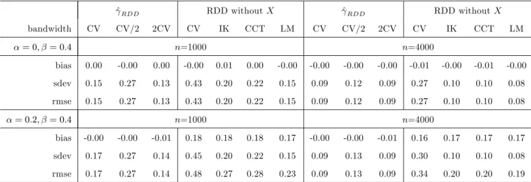
Table 1: Simulations - sharp RDD ^RDD RDD without X ^RDD RDD without X bandwidth CV CV/2 2CV CV IK CCT LM CV CV/2 2CV CV IK CCT LM = 0; = 0:4 n=1000 n=4000 bias 0.00 -0.00 0.00 -0.00 0.01 0.00 -0.00 -0.00 -0.00 -0.00 -0.01 -0.00 -0.01 -0.00 sdev 0.15 0.27 0.13 0.43 0.20 0.22 0.15 0.09 0.12 0.09 0.27 0.10 0.10 0.08 rmse 0.15 0.27 0.13 0.43 0.20 0.22 0.15 0.09 0.12 0.09 0.27 0.10 0.10 0.08 = 0:2; = 0:4 n=1000 n=4000 bias -0.00 -0.00 -0.01 0.18 0.18 0.18 0.17 -0.00 -0.00 -0.01 0.16 0.17 0.17 0.17 sdev 0.17 0.27 0.14 0.45 0.20 0.22 0.15 0.09 0.13 0.09 0.30 0.10 0.10 0.08 rmse 0.17 0.27 0.14 0.48 0.27 0.28 0.23 0.09 0.13 0.09 0.34 0.20 0.20 0.19

Note: ‘CV’, ‘CV/2’, ‘2CV’ stands for bandwidth selection based on least squares cross-validation, as well as twice and half that value. ‘IK’ is the optimal Imbens-Kalyanaraman (2012) bandwidth. ‘CCT’ is the robust inference approach of Calonico, Cattaneo, and Titiunik (2014) (CCT). ‘LM’is the local cross-validation approach of Ludwig and Miller (2007) based on the median values of the running variable above and below the threshold. ‘bias’, ‘sdev’, and ‘rmse’ report the bias, standard deviation, and root mean squared error of the respective method.

and Titiunik (2014) (CCT) as implemented as default option in the ‘rdrobust’ package for ‘R’ by Calonico, Cattaneo, and Titiunik (2015); and the local cross-validation approach of Ludwig and Miller (2007) (LM) based on the median values of the running variable above and below the threshold. In all estimations, the Epanechnikov kernel is used.

Table 1 reports the bias, standard deviation, and root mean squared error (RMSE) of the estimators for various choices of ; in the sharp RDD. When setting = 0; = 0:4, all procedures are unbiased as expected. Under either sample size, ^_RDD outperforms RDD without X in terms of precision when using the same CV bandwidth for both estimators. Furthermore, ^_RDD with CV is in most cases also more precise than RDD without X based on the IK, CCT, and LM bandwidths.31 As expected, a smaller bandwidth (CV/2) increases

3 1

Under n = 1000; = 0; = 0:4, the means (standard deviations) of the CV, IK, CCT, and LM bandwidths for Z are 0.16 (0.06), 0.84 (0.29), 0.66 (0.11), 1.58 (0.51), respectively. The means and standard deviations are

the standard deviation of ^_RDD, while a larger bandwidth (2CV) slightly decreases it. For n = 4000, however, the di¤erences in precision are quite moderate for various bandwidth choices.

When setting = 0:2 and = 0:4, the biases of ^_RDD are again close to zero, while this is no longer the case for RDD without X. For n = 1000, ^_RDD with CV and 2CV dominates any RDD without X in terms of bias, standard deviation, and root mean squared error (RMSE), while ^_RDD with CV/2 is less precise. Under n = 4000, all three versions of ^_RDD have a considerably smaller RMSE than any RDD without X.

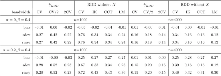
Table 2: Simulations - fuzzy RDD

^RDD RDD without X ^RDD RDD without X bandwidth CV CV/2 2CV CV IK CCT LM CV CV/2 2CV CV IK CCT LM = 0; = 0:4 n=1000 n=4000 bias -0.01 0.00 -0.02 -0.05 -0.02 -0.01 -0.01 0.01 -0.00 0.01 -0.01 0.00 -0.01 -0.01 sdev 0.27 0.42 0.22 0.76 0.34 0.34 0.24 0.16 0.18 0.14 0.34 0.16 0.16 0.12 rmse 0.27 0.42 0.22 0.76 0.34 0.34 0.24 0.16 0.18 0.14 0.34 0.16 0.16 0.12 = 0:2; = 0:4 n=1000 n=4000 bias -0.01 -0.00 -0.03 0.25 0.27 0.27 0.27 0.01 0.01 0.00 0.25 0.28 0.27 0.27 sdev 0.28 0.52 0.23 0.67 0.33 0.34 0.23 0.15 0.20 0.15 0.39 0.16 0.16 0.12 rmse 0.28 0.52 0.23 0.72 0.43 0.43 0.36 0.15 0.20 0.15 0.46 0.32 0.31 0.30

Note: ‘CV’, ‘CV/2’, ‘2CV’ stands for bandwidth selection based on least squares cross-validation, as well as twice and half that value. ‘IK’ is the optimal Imbens-Kalyanaraman (2012) bandwidth. ‘CCT’ is the robust inference approach of Calonico, Cattaneo, and Titiunik (2014) (CCT). ‘LM’is the local cross-validation approach of Ludwig and Miller (2007) based on the median values of the running variable above and below the threshold. ‘bias’, ‘sdev’, and ‘rmse’ report the bias, standard deviation, and root mean squared error of the respective method.

Secondly, we consider the case of a fuzzy RDD. We modify the DGP by replacing D = IfZ > 0g in (19) with D = If 1 + 2IfZ > 0g + 0:5U + Q > 0g, with Q N (0; 1) independently of any other variable. D is now endogenous even at the threshold due to U entering both

the treatment and outcome equation. The bandwidths used for the estimation of d+(x; z) and d (x; z) required for the fuzzy RDD method are selected in an analogous way as for m+(x; z) and m (x; z). We also consider fuzzy RDD estimation without covariates based on Dimmery (2016) with CV, IK, CCT, and LM bandwidth choices, repectively.32 The results are reported in Table 2 and show a qualitatively similar pattern as for the sharp RDD. However, standard errors are generally larger as estimation is based on the compliers only, which by the de…nition of the DGP make up for about 65% of the population.

5

Application

As an empirical illustration of our method we use data from Lalive (2008), who studies a la-bor market program introduced in June 1988 that extended the maximum duration of unem-ployment bene…ts from 30 to 209 weeks for job seekers aged 50 or older in certain regions of Austria under particular conditions. This suggests the use of a sharp RDD for assessing the program’s e¤ect on labor market outcomes such as unemployment duration. The treatment is de…ned based on the age threshold of 50. As acknowledged by Lalive (2008), however, a concern is that employees and companies could manipulate age at entry into unemployment, for example, by postponing a layo¤ in a way that the age requirement is just satis…ed. This is a common concern in many applications. If such manipulations are selective with respect to employee characteristics that also a¤ect labor market outcomes, conventional RDD without covariates fails to identify the e¤ect of the program due to confounding related to an imbal-ance of the characteristics around the threshold. In contrast, our method remains consistent if all labor market relevant characteristics are plausibly observed in the data. As a word of caution, however, we would like to point out that this cannot be taken for granted in our ap-plication. For instance, unobserved individual characteristics like motivation, (dis-)utility from work, and self-con…dence might predict both manipulation and labor market success. To con-sistently estimate the program e¤ect by our method, it is required that these factors do not

3 2_{Under n = 1000; = 0; = 0:4, the means (standard deviations) of the CV, IK, CCT, and LM bandwidths}

for Z are 0.23 (0.07), 0.84 (0.29), 0.66 (0.11), 1.73 (0.59), respectively. The means and standard deviations are very similar under n = 1000; = 0:2; = 0:4.

entail confounding conditional on the socio-economic and employment-related characteristics available in the data (see the discussion below).

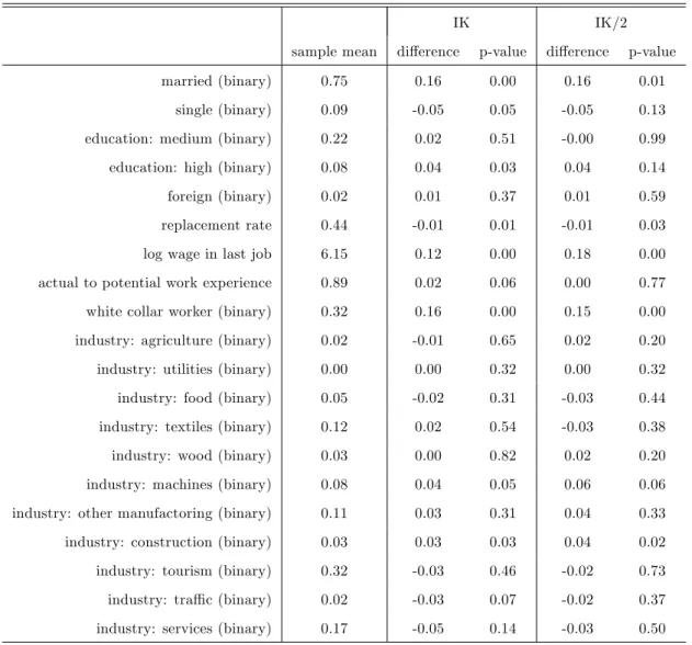
Table 3: Covariate sample means and balance tests at the threshold

IK IK/2

sample mean di¤erence p-value di¤erence p-value

married (binary) 0.75 0.16 0.00 0.16 0.01

single (binary) 0.09 -0.05 0.05 -0.05 0.13

education: medium (binary) 0.22 0.02 0.51 -0.00 0.99

education: high (binary) 0.08 0.04 0.03 0.04 0.14

foreign (binary) 0.02 0.01 0.37 0.01 0.59

replacement rate 0.44 -0.01 0.01 -0.01 0.03

log wage in last job 6.15 0.12 0.00 0.18 0.00

actual to potential work experience 0.89 0.02 0.06 0.00 0.77

white collar worker (binary) 0.32 0.16 0.00 0.15 0.00

industry: agriculture (binary) 0.02 -0.01 0.65 0.02 0.20

industry: utilities (binary) 0.00 0.00 0.32 0.00 0.32

industry: food (binary) 0.05 -0.02 0.31 -0.03 0.44

industry: textiles (binary) 0.12 0.02 0.54 -0.03 0.38

industry: wood (binary) 0.03 0.00 0.82 0.02 0.20

industry: machines (binary) 0.08 0.04 0.05 0.06 0.06

industry: other manufactoring (binary) 0.11 0.03 0.31 0.04 0.33

industry: construction (binary) 0.03 0.03 0.03 0.04 0.02

industry: tourism (binary) 0.32 -0.03 0.46 -0.02 0.73

industry: tra¢ c (binary) 0.02 -0.03 0.07 -0.02 0.37

industry: services (binary) 0.17 -0.05 0.14 -0.03 0.50

Note: ‘IK’, ‘IK/2’denote the optimal Imbens-Kalyanaraman (2012) bandwidth and half that value in an RDD estimation when using each of the covariates as outcome. P-values are based on analytic standard errors and account for clustering of age (measured in months).

Our analysis makes use of the Austrian social security database, which includes information on job seekers (age, employment, unemployment and earnings history) and the employers (region and industry), and the Austrian unemployment register, which contains information on the place of residence and socio-economic characteristics. The universe of in‡ows into

unemployment between 1986 and 1995 is covered, and the in‡ow sample can be followed up until the end of 1998. We refer to Lalive (2008) for a description of sample adjustments made to the data set. Speci…cally, we consider the female subsample in the age bracket 46 to 53 years living in a region where the program had been introduced, consisting of 5659 observations. The outcome variable Y is unemployment duration, measured as weeks registered at the unemployment o¢ ce. The running variable Z is distance to the age threshold of 50, measured in months divided by 12. Table 3 reports sample means and balancing tests at the threshold for potentially labor market relevant characteristics, which serve as X. The tests are based on running RDD estimations with the elements in X as outcome variables using the ‘rdd’ package, which performs local linear regression around the threshold. Estimates, standard errors, and p-values are reported for the IK bandwidth and half of it. Indeed, several covariates are imbalanced around the threshold, which concerns among others marital status, wage in the last job, and being a white collar worker.33 The results therefore suggest that observations slightly above the age threshold have somewhat more favorable labor market relevant characteristics than those slightly below.

Our RDD estimator derived from equation (7) controls for di¤erences in X by giving appropriate weights to each of these characteristics, according to their distribution about the thresh-old. Consider, for example, the variable marital status, which is signi…cantly di¤erent in Table 3. On average, 75% of the observations in the sample are married, but the (conditional) probability of being married is discontinuous at the threshold: The nonparametric estimates of the probability from the left and right are 63.7% and 79.9%, respectively. In a symmetric neighbourhood about the threshold, the probability of being married is thus 71.8%. Our method proceeds by estimating the outcome unemployment duration for married women left and right of the threshold and multiplying with a weight of 0.718. An analogous approach applies to unmarried women using a weight of 0.282.

3 3

To control the family-wise error rate of multiple testing in Table 3, one may apply the (conservative) Bonferroni correction: divide the nominal level of signi…cance by the number of tested covariates (in our case 20) and reject an individual null hypothesis of covariate balance if the corresponding p-value is even lower. For log wage in last job and white collar worker, the null hypothesis is rejected under either bandwidth at the nominal 5% level of signi…cance.

Hence, a weighted average with respect to the fraction of married women in a symmetric neighbourhood about the threshold is taken. This removes the discontinuity in marital status: The 63.7% married women to the left are up-weighted with 0.718/0.637, while the 79.9% married women to the right are down-weighted with 0.718/0.799. Accordingly, the 36.3% unmarried women to the left are down-weighted with 0.282/0.363, while those 20.1% to the right are up-weighted with 0.282/0.201. In contrast, RDD estimation not controlling for X compares the unemployment duration left and right of the threshold without weighting, thereby ignoring that there are for instance fewer married women to the left than to the right of the threshold.

Table 4 presents the results for ^_RDD when using cross-validation for the bandwidth se-lection of hx; hz in the …rst step estimation of m+ and m . Di¤erent from the simulations

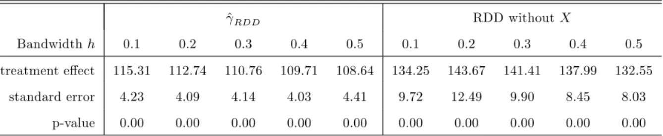
in Section 4, however, the covariates now contain both continuous and discrete elements. We therefore apply the method of Racine and Li (2004), which allows for both continuous and discrete regressors by means of product kernels and is implemented in the ‘np’package of Hay-…eld and Racine (2008). We use the Epanechnikov, Wang and van Ryzin (1981), and Aitchison and Aitken (1976) kernel functions for continuous, ordered discrete, and unordered discrete co-variates, respectively. We consider several choices for bandwidth h in the Epanechnikov-based boundary kernel function for the running variable in (13): 0.1, 0.2,..., 0.5. We also compare the results to RDD regression without covariates based on the ‘rdd’ package with the same bandwidth choice h. The standard errors of any method are based on nonparametrically boot-strapping the respective estimates 999 times, i.e. randomly resampling the original data with replacement and applying the estimators to the bootstrap samples. The ^_RDD estimates point to a substantial increase in unemployment duration by about 110 weeks.

The results are highly signi…cant, as the standard errors of roughly 4 weeks are quite moderate. When using RDD without X, both the e¤ect of about 140 weeks and the standard error of about 10 weeks are substantially higher. For each bandwidth value considered, the estimates are statistically signi…cantly di¤erent between the methods (at the 5% level based on bootstrapping the di¤erences in the estimates 999 times). This indicates that there might be some confounding due to observed covariates. Also the e¤ects reported in Table 3 columns (3)

Table 4: E¤ect estimates ^RDD RDD without X Bandwidth h 0.1 0.2 0.3 0.4 0.5 0.1 0.2 0.3 0.4 0.5 treatment e¤ect 115.31 112.74 110.76 109.71 108.64 134.25 143.67 141.41 137.99 132.55 standard error 4.23 4.09 4.14 4.03 4.41 9.72 12.49 9.90 8.45 8.03 p-value 0.00 0.00 0.00 0.00 0.00 0.00 0.00 0.00 0.00 0.00

Note: The bandwidths hx; hzfor the …rst step estimates of m+and m entering ^RDD(see Section 3) are picked

by least squares cross-validation. For bandwidth h on the running variable Z in ^_RDD and RDD without X, several values are considered as indicated in the table. Standard errors are based on bootstrapping the estimate 999 times. Sample size is 5659 observations. X includes the variables given in Table 3: marital status, education, migration status, replacement rate, log wage in last job, actual to potential work experience, white collar worker, and industry.

and (4) of Lalive (2008) when omitting X and either using a global RDD model with a higher order polynomial for the running variable or a local linear model with a very small bandwidth are somewhat higher than ^_RDD (122 to 126 weeks). In contrast, the e¤ect of 103 weeks presented in column (6) of Table 3 in Lalive (2008) is based on linearly controlling for covariates. Our somewhat higher (and at the 5% level statistically signi…cantly di¤erent) estimates (when bootstrapping the di¤erences) are likely due to using a more ‡exible speci…cation with respect to the association of Y and X.

6

Conclusion

In this paper, the regression discontinuity design (RDD) has been generalized to incorporate covariates X in a fully nonparametric way. Including covariates can reduce the variance and eliminate biases if X is discontinuously distributed at the threshold. It has been shown that the curse of dimensionality does not apply and that the average treatment e¤ect (on the local compliers) can be estimated at rate n 25 irrespective of the dimension of X. For achieving

properties of our estimator in simulations and applied it to estimate the e¤ect of age-dependent unemployment bene…ts on unemployment duration in Austrian labor market reform, where manipulation at the threshold is a potential concern.

References

Aitchison, J., and C. Aitken (1976): “Multivariate binary discrimination by the kernel method,” Biometrika, 63, 413–420.

Battistin, E.,andE. Rettore (2008): “Ineligibles and eligible non-participants as a double comparison group in regression-discontinuity designs,” Journal of Econometrics, 142, 715– 730.

Black, D., J. Galdo,and J. Smith (2007): “Evaluating the regression discontinuity design using experimental data,” mimeo, University of Michigan, USA.

Calonico, S., M. D. Cattaneo, M. H. Farrell, and R. Titiunik (2016): “Regression Discontinuity Designs Using Covariates,” working paper, University of Michigan.

Calonico, S., M. D. Cattaneo, and R. Titiunik (2014): “Robust Nonparametric Con…-dence Intervals for Regression-Discontinuity Designs,” Econometrica, 82, 2295–2326.

(2015): “rdrobust: An R Package for Robust Nonparametric Inference in Regression-Discontinuity Designs,” R Journal, 7, 38–51.

de Chaisemartin, C. (2016): “Tolerating de…ance? Identi…cation of treatment e¤ects without monotonicity,” working paper, University of Warwick.

Dimmery, D. (2016): “Package ‘rdd’,” Manual for the statistical software ‘R’.

Dong, Y. (2014): “An Alternative Assumption to Identify LATE in Regression Discontinuity Designs,” Unpublished Manuscript, University of California Irvine.

Eugster, B., R. Lalive, A. Steinhauer,andJ. Zweimüller (2017): “Culture, Work At-titudes and Job Search: Evidence from the Swiss Language Border,”forthcoming in Journal of the European Economic Association.

Fisher, R. (1935): Design of Experiments. Oliver and Boyd, Edinburgh.

Frandsen, B., M. Frölich, and B. Melly (2012): “Quantile treatment e¤ects in the regression discontinuity design,” Journal of Econometrics, 168 (2), 382–395.

Frölich, M., and B. Melly (2013): “Unconditional quantile treatment e¤ects under endo-geneity,” Journal of Business and Economic Statistics (JBES), 31:3, 346–357.

Frölich, M. (2007): “Nonparametric IV Estimation of Local Average Treatment E¤ects with Covariates,” Journal of Econometrics, 139, 35–75.

Gasser, T., andH. Müller (1979): “Kernel estimation of regression functions,”in Smooth-ing techniques for curve estimation, Lecture Notes in Mathematics 757, ed. by T. Gasser,