On the relationship between empirical likelihood and empirical saddlepoint approximation for multivariate M-estimators

Printed in Great Britain

On the relationship between empirical likelihood and empirical

saddlepoint approximation for multivariate M-estimators

BY ANNA CLARA MONTI

Centro di Specializzazione e Ricerche Economico-agrarie per il Mezzogiorno, Via Universita 96, 80055 Portia (Napoli), Italy

AND ELVEZIO RONCHETTI

Faculty of Economic and Social Sciences, University of Geneva, CH-1211 Geneva, Switzerland

SUMMARY

By comparing the expansions of the empirical log-likelihood ratio and the empirical cumulant generating function calculated at the saddlepoint, we investigate the relationship between empirical likelihood and empirical saddlepoint approximations. This leads to a nonparametric approximation of the density of a multivariate M-estimator based on the empirical likelihood and, on the other hand, it provides nonparametric confidence regions based on the empirical cumulant generating function. Some examples illustrate the use of the empirical likelihood in saddlepoint approximations and vice versa.

Some key words: Empirical bootstrap likelihood; Empirical likelihood; Influence function; M-estimator;

Nonparametric confidence regions; Saddlepoint approximation; Small sample asymptotics.

1. I N T R O D U C T I O N

The purpose of this paper is to discuss the relationship between empirical likelihood techniques and empirical saddlepoint approximations for multivariate M-estimators. Owen (1988, 1990) defined an empirical version of the likelihood ratio and showed how it can be used to construct nonparametric confidence regions. In particular, he showed that, as in the parametric case, minus twice the empirical log-likelihood ratio has asymptotically a x1 distribution. DiCiccio, Hall & Romano (1989), DiCiccio & Romano

(1989) and Hall (1990) investigated further the relationship between empirical likelihood and the parametric theory. For instance, they showed that a Bartlett correction can be applied to the empirical likelihood. Finally, Hall & La Scala (1990) give a review of the methodology and the algorithms, and Davison, Hinkley & Worton (1992) show the relationship with bootstrap likelihoods.

Saddlepoint approximations in statistics go back to Daniels (1954). These techniques provide very accurate approximations of the distribution of some statistic even in small samples. For a review, see Reid (1988), Barndorfl-Nielsen & Cox (1989, Ch. 4,6) and Field & Ronchetti (1990). The construction of these approximations typically requires knowledge of the underlying distribution F of the observations but one can make these techniques nonparametric by replacing F by the empirical distribution function. This can be viewed as a way to avoid resampling by approximating the bootstrap distribution by means of saddlepoint techniques; see Davison & Hinkley (1988), Feuerverger (1989), Young & Daniels (1990), Wang (1990) and Ronchetti & Welsh (1993).

In § 2 we summarize the results based on the empirical saddlepoint approximation. In order to show the relationship between empirical likelihood techniques and empirical saddlepoint approximations, we compare in § 3 the expansions of minus twice the empirical log-likelihood ratio W(t) and the empirical cumulant generating function K(t) for a general multivariate M-estimator. Here K(t) = In [n~l 1 exp {a(tyip(xh <)}], where

x , , . . . , xn are observations from a random sample, a(t) is the saddlepoint which solves

equation (5) below, and (/>(*» 0 is the vector function which defines the M-estimator. The relation is

nK(t) = -£lV(0+*n-

r(u) + 0 ( 0 , (D

and depending on the third moment of the influence function of the M-estimator. This formula allows one to translate between empirical likelihood ratios and saddlepoint densities by making a skewness correction and incurring a loss of accuracy of O(n~l).

This relationship holds generally for a statistic admitting an influence function. Moreover, the connection between the saddlepoint and the first derivative of the empirical likelihood can be related to a result by DiCiccio, Field & Fraser (1990). Finally in § 4, some examples illustrate the use of the empirical likelihood in saddlepoint approximations and vice versa.

2. THE EMPIRICAL SADDLEPOINT APPROXIMATION

Let x , , . . . , xn be n independent and identically distributed random variables with

distribution F depending on a k- vector parameter 8 belonging to some parametric space 0 . An M-estimator for 6 is a statistical functional defined as a root Tn of 1 <M*i» Tn) = 0,

where the summation is over the range i = l,...,n. Under the conditions (i)-(v) of Ronchetti & Welsh (1993), the empirical saddlepoint approximation of the density of Tn

at t = Tn + n~^u is given by

det {JCXOr'ldet {A(t)}\ exp {nK(t)}, (2) where

k{t) = In [iT

£ exp {a(0>(*,, 0)1, (3)

L (-i J

£ at/>(3X'>0exp{a(0V(^,0K (4) i-i at

i-i

and a(t) satisfies

(5)

I - I

Formula (2) can be viewed as an approximation of the bootstrap distribution which does not require resampling; see Davison & Hinkley (1988) and Ronchetti & Welsh (1993).

Empirical likelihood and empirical saddlepoint 331 In order to compare the empirical saddlepoint approximation with the empirical likelihood, we consider the following expansion of K(t) (see Appendix):

) + O(n~\ (6) where V' = A(Tn)~i2.+{A(Tn)'}~1 is the estimated asymptotic covariance matrix of TH,

! ' I

*,

T

)',

1 - 1 dt B(u) is a fcx/c matrix with elements

B(u)u = n ( - 1 r - l Pjjx,, t) Oh c(u) is a fc-vector, n k k

_*,,

₀

and I F ( X , ; TH) = -A(Tn)~1ij/(xl, Tn) is the influence function of Tn (Hampel, 1974). In

the case of a univariate M-estimator, (6) becomes

dt , _i/2u3A(Tn) _, -- 5 " — 5 n L at' n-\ (8) where •u rny 372

is the third empirical cumulant of if/(x, t), given t = Tn. Moreover, if Tn is the univariate

mean x, then A(Tn) = - 1 and (8) simplifies further to

Kit) = -\n~x (9)

with

Notice that in this case -nK(t) = /EB(0. the bootstrap likelihood of Davison et al. (1992, eqn (4-8)), where saddlepoint approximations are applied in place of resampling to compute a bootstrap likelihood. Therefore,

In the notation of Davison et al. (1992), ^ = u/i*, KO,O = £ , KO,O,O = y£3 / 2 and our (10) corresponds to their (7-10) except that in (7-10) all signs must be reversed and the coeflBcient \ in the term of order n- i must be changed to \.

In the next section, (6) will be compared to the expansion of the empirical log-likelihood ratio.

3. SADDLEPOINT APPROXIMATION THROUGH EMPIRICAL LIKELIHOOD

The empirical likelihood ratio is a test variable which leads to the construction of confidence regions in a nonparametric framework (Owen, 1988, 1990). The value t is included in the confidence region for 6 if, according to the value of the empirical likelihood ratio, the hypothesis Ho: 6 = t cannot be rejected. Formally, the empirical likelihood

ratio is the ratio between the nonparametric estimate of the maximum of the likelihood function under the hypothesis Ho and the nonparametric estimate of the maximum of

the likelihood function without restrictions. Since the maximum of the nonparametric likelihood function under no restriction is n~", the empirical likelihood ratio is given by:

where the pr weights satisfy

(i) p,»Q, V/,

(ii) tpi = h

( - 1

A Lagrangian argument leads to

W(t) = -2 In i(t) = 2 £ In {1 + | ( 0 > ( * i , ' ) } , where g(t) satisfies

> 0 =0. (11) The Lagrangian multiplier ^(f) plays the same role in the construction of the empirical likelihood ratio as the saddlepoint a(t) in the empirical saddlepoint approximation. In fact, for any t e 0, the empirical likelihood ratio requires the computation of the weights p, which centre the empirical distribution at t.

Applying the same algebra of the Appendix yields in the same notation

~3 / 2) , (12)

/-i

and replacing (12) in the Taylor expansion of W(t) gives

MTn)u

Empirical likelihood and empirical saddlepoint 333 In case of a univariate M-estimator (13) reduces to

2 _tu A ( r j . _ 5" —^372—r* + O(" ) and, for tp(x, t) = x-t,

Owen (1988) proved that W(t) is asymptotically distributed as a ^ i . Thus, asymptotic confidence regions with nominal coverage probability 1 - e can be constructed as

}, (14) where x\,\-t is the 100(1 — e) percentile of the xl distribution.

We are now able to establish the connections between the empirical likelihood and the empirical saddlepoint approximation. In fact, by a comparison of (6) and (13) we obtain formula (1),

where T(u) is defined by (7).

More generally, equation (1) holds for any multivariate statistic admitting an influence function by replacing the function \p in K by the influence function of the statistic.

Relation (1) can be used in two ways. First, we can obtain a nonparametric approxima-tion of the density of Tn directly from the empirical log-likelihood ratio by replacing

nK{t) by -jW(t) + zn~^T(u) in the empirical saddlepoint approximation. Secondly, we can construct nonparametric confidence regions by replacing W(t) in (14) by -2nK(t) + jn~^r(u). Both methods involve solving a set of equations, that is (5) and (11). In general these are of the same computational complexity. However, if one set of equations is harder to solve in a specific situation, then relation (1) allows us to use the other set as an approximation. From a conceptual viewpoint, the possibility to use the empirical likelihood to approximate the density of an estimator is attractive. This is in fact a nonparametric extension of the well known relationship between the likelihood function and the density of the maximum likelihood estimator in a parametric setup as given by Barndorfl-Nielsen (1983).

Notice that the correction term in (1) depends on the skewness of IF (X; t), for t = Tn.

In the univariate case, n~4r(u) = - u3 V~3/2a, where

A

'

is the nonparametric estimator of the acceleration constant appearing in the BCa method of Efron (1987, eqn (7.3), p. 178). If IF(X; Tn) has a symmetric distribution, nK(t) =

-\W(t) + O(n~l). In the case of the mean, (1) gives the correction term for the empirical

bootstrap likelihood /EB(0 to be at distance O(n~l) from the empirical log-likelihood ratio.

There is another point to be highlighted. If we look at (3)-(4) we notice that

and replacing (1) we have

at at

Similar algebra shows that the same relationship holds between a(t) and K(t) in the parametric saddlepoint approximation based on the true underlying distribution F as given by Field (1982). Since

we obtain

at (15)

This generalizes the remark on p. 94 of DiCiccio et al. (1990) that the role of the saddlepoint is being played by the first derivative of the log-likelihood function.

4. EXAMPLES

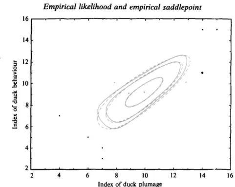
In this section we discuss four examples which illustrate the use of relationship (1). Example 1: Duck data. We first consider the duck data taken from Larsen & Marx (1986, p. 440). It is a data set of 10 bivariate observations, where the first variable is an index of duck plumage and the second one an index of duck behaviour. Figure 1 compares the contours of empirical likelihood and normal likelihood confidence regions following Owen (1990). In Fig. 2, instead, we compare the empirical likelihood confidence regions with the saddlepoint based confidence regions. The latter are obtained by using (14),

8 10 Index of duck plumage

12 14 16

Fig. 1. 50%, 95%, 99% contours of ordinary empirical likelihood (unbroken) and normal likelihood (broken) confidence regions for duck data.

Empirical likelihood and empirical saddlepoint ₃₃₅

12 14 16

6 8 10 Index of duck plumage

Fig. 2. 50%, 95%, 99% contours of ordinary (unbroken) and saddlepoint (broken) empirical likelihood confidence regions for duck data.

where W(t) is replaced by -2nK(t). This plot shows that even without correction term the saddlepoint based confidence regions are very close to the empirical likelihood regions. Example 2: Bootstrap percentiles ofX-fifor the data of Davison & Hinkley (1988). Davison & Hinkley (1988, pp. 419-20) compared two approximations for the percentage points of X-fi for a sample of size 10. They considered the empirical saddlepoint approximation and a bootstrap approximation based on 50 000 replicates. We report their numbers in the second and third column of Table 1. The fourth column gives the saddlepoint approximation obtained by replacing nK(t) by -jW(t)+in~^u31~3/2y as

given in (1) and (9). It can be seen that the accuracy of this approximation is nearly the same as that of the original saddlepoint approximation.

Table 1. Approximations to percentage points of X-fi., Example 2.

Data of Davison & Hinkley (1988)

obability 0001 0005 0010 0050 0100 0-900 0-950 0-990 0-995 0-999 Bootstrap -5-55 -4-81 -4-42 -3-34 -2-69 2-87 3-73 5-47 612 7-52 Empirical saddlepoint -5-52 -4-81 -4-43 -3-33 -2-69 2-85 3-75 5-48 6-12 7-46 Empirical likelihood -5-32 -4-59 -4-19 - 3 0 5 -2-39 2-95 3-73 5 1 7 5-68 6-70 Bootstrap approximations based on 50 000 resamplings.

Example 3: The distribution of the Huber estimator under contaminated data. We consider an approximation of the distribution of the Huber estimator based on 10 independent and identically distributed observations from the contaminated normal distribution 0-95 x N ( 0 , l) + OO5x7V(O, 32). The Huber estimator is an M -estimator with «/»(*, 0 = (x — t) min (1, c/\x —1\) for some positive constant c. We choose here c = 1-4. Since the score function \\i is bounded, this estimator is robust against outlying observations and long-tailed underlying distributions. Table 2 compares the exact tail areas and those obtained by using the empirical saddlepoint and the empirical likelihood approximations. The 'exact' tail areas were obtained by a simulation on 30 000 samples. The empirical saddlepoint approximation was obtained by first computing the density /n(f) given by (2) on a grid of points tj at a distance 0-02 from each other. The tail areas were estimated by

The numbers given in the third and fourth columns of Table 2 are averages over 200 samples. The empirical likelihood approximation is computed as the empirical saddle-point approximation except that nK(t) is replaced by — \W(t). Table 2 shows that the empirical saddlepoint approximation is more accurate for tail areas between 1% and 4% while the empirical likelihood approximation outperforms the former in the range

Table 2. Tail areas of the Huber estimator, Example 3 c = 1 -4, X, ~ 0-95 x N{0, 1) + 0-05 x N(0, 32) t 0-44 0-52 0-58 0-64 0-70 0-76 0-82 Exact 0102 0069 0049 0 034 0023 0016 0010 Empincal saddlepoint 0-078 0051 0-037 0-027 0019 0014 0010 Empincal likelihood 0-099 0071 0055 0-042 0033 0025 0019

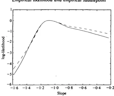
Example 4: Gesell adaptive score data. The data set is taken from Mickey, Dunn & Clark (1967) and Rousseeuw & Leroy (1987, p. 46). The Gesell adaptive score for 21 children is given with the age, in months, at which a child utters its first word. Mickey et al. (1967) found that observation 19 is an outlier, so a robust analysis is appropriate. We first centred the x's and y's with respect to their medians (Table 3). Then we performed a robust regression of y versus x by estimating the slope by a^Huber estimator with c = 1-4. Figure^3 compares the empirical log-likelihood ratio - 5 ^ ( 1 ) as given by Owen (1991) with nK(t). Again the two curves are very close.

Table 3. Gesell adaptive score data (centred), Example 4 X y X y 4 0 - 2 1 15 - 2 4 - 1 - 1 2 - 1 - 1 2 0 - 1 1 - 2 - 4 0 7 4 7 - 1 5 9 - 8 1 10 7 - 2 31 - 3 8 0 5 6 26 - 3 9 0 - 9 9 - 1 - 1 5 - 4 18

Empirical likelihood and empirical saddlepoint 337

-1-6 - 1 - 4 -1-2 - 1 0 -0-8 -0-6 - 0 - 4 - 0 - 2

Fig. 3. Approximation of the log-likelihood of the regression coefficient in the data set of Rousseeuw & Leroy (1987) through

~{W(t) (unbroken) and nK(t) (broken).

A C K N O W L E D G E M E N T S

The research of the first author was partially supported by C.N.R. The authors are grateful to the editor and the referees for their comments which led to an improved exposition.

APPENDIX

Derivation of the expansion (6)

First consider the saddlepoint a(t). Applying the implicit function theorem in (5) yields a(t) = O(n~i). Thus we have

Writing a(t) = al(t)+a2(t), we get at(t)+a2{t) in (5) gives

Thus

) = -n'!ll~iA(Tn)u and a2(t) = O(n'1). Replacing a{t) =

?+(x

7

)J

Substituting the expansion for a(t) in (2) and expanding K(t), we obtain K(t) = \

REFERENCES

B A R N D O R F F - N I E L S E N , 0. E. (1983). On a formula forthe distribution of the maximum likelihood estimator.

Biometrika 70, 343-65.

B A R N D O R F F - N I E L S E N , O. E. & C o x , D. R. (1989). Asymptotic Techniques for Use in Statistics. London: Chapman and Hall.

D A N I E L S , H. E. (1954). Saddlepoint approximation in statistics. Ann. Math. Statist. 25, 631-50.

D A V I S O N , A. C. & H I N K L E Y , D. V. (1988). Saddlepoint approximations in resampling methods. Biometrika 75, 417-31.

D A V I S O N , A. C , H I N K L E Y , D. V. & WORTON, B. J. (1992). Bootstrap likelihoods. Biometrika 79, 113-30. D I C I C C I O , T. J., FIELD, C. A. & FRASER, D. A. S. (1990). Approximations of marginal tail probabilities

and inference for scalar parameters. Biometrika 77, 77-95.

D I C I C C I O , T. J., HALL, P. & R O M A N O , J. P. (1989). Comparison of parametric and empirical likelihood functions. Biometrika 76, 465-76.

D I C I C C I O , T. J. & R O M A N O , J. P. (1989). On adjustments to the signed root of the empirical likelihood ratio statistics. Biometrika 76, 447-56.

E F R O N , B. (1987). Better bootstrap confidence intervals (with discussion). J. Am. Statist. Assoc 82, 171-200. FEUERVERGER, A. (1989). On the empirical saddlepoint approximation. Biometrika 76, 457-64.

FIELD, C. A. (1982). Small sample asymptotic expansions for multivariate M-estimates. Ann. Statist. 10, 672-89.

FIELD, C. A. & RONCHETTI, E. (1990). Small Sample Asymptotics. Hayward, CA: Inst. Math. Statist Monograph Series.

HALL, P. (1990). Pseudo likelihood theory for empirical likelihood. Ann. Statist. 18, 121-40.

HALL, P. & L A SCALA, B. (1990). Methodology and algorithms of empirical likelihood. Int. Statist. Rev. 58, 109-27.

HAMPEL, R. R. (1974). The influence curve and its role in robust estimation. J. Am. Statist. Assoc 69, 383-93. LARSEN, R. J. & MARX, M. L. (1986). An Introduction to Mathematical Statistics and its Applications.

Englewood Cliffs, NJ: Prentice-Hall.

M I C K E Y , M. R., D U N N , O. J. & CLARK, V. (1967). Note on the use of stepwise regression in detecting outliers. Comp. Biomed. Res. 1, 105-111.

O W E N , A. B. (1988). Empirical likelihood ratio confidence intervals for a single functional. Biometrika 75, 237-49.

O W E N , A. B. (1990). Empirical likelihood ratio confidence regions. Ann. Statist. 18, 90-120. O W E N , A. B. (1991). Empirical likelihood for linear models. Ann. Statist. 19, 1725-47. R E I D , N. (1988). Saddlepoint methods and statistical inference. Statist. Sri. 3, 213-38.

RONCHETTI, E. & WELSH, A. H. (1993). Empirical saddlepoint approximations for multivariate M-estimators. J. R. Statist Soc B. To appear.

ROUSSEEUW, P. & LEROY, A. (1987). Robust Regression and Outlier Detection. New York: Wiley. W A N G , S. (1990). Saddlepoint approximations in resampling analysis. Ann. Inst Statist. Math. 42, 115-31. Y O U N G , G. A. & D A N I E L S , H. E. (1990). Bootstrap bias. Biometrika TJ, 179-85.