HAL Id: hal-01381781
https://hal.inria.fr/hal-01381781v2
Submitted on 22 Nov 2018
HAL is a multi-disciplinary open access
archive for the deposit and dissemination of
sci-entific research documents, whether they are
pub-lished or not. The documents may come from
teaching and research institutions in France or
abroad, or from public or private research centers.
L’archive ouverte pluridisciplinaire HAL, est
destinée au dépôt et à la diffusion de documents
scientifiques de niveau recherche, publiés ou non,
émanant des établissements d’enseignement et de
recherche français ou étrangers, des laboratoires
publics ou privés.
A Multi-Criteria Experimental Ranking of Distributed
SPARQL Evaluators
Damien Graux, Louis Jachiet, Pierre Genevès, Nabil Layaïda
To cite this version:
Damien Graux, Louis Jachiet, Pierre Genevès, Nabil Layaïda. A Multi-Criteria Experimental Ranking
of Distributed SPARQL Evaluators. Big Data 2018 - IEEE International Conference on Big Data,
Dec 2018, Seattle, United States. pp.1-10. �hal-01381781v2�
A Multi-Criteria Experimental Ranking of
Distributed SPARQL Evaluators
Damien Graux
§‡, Louis Jachiet
†‡, Pierre Genev`es
‡, Nabil Laya¨ıda
‡§
Enterprise Information Systems, Fraunhofer IAIS – Sankt Augustin, Germany
†D´epartement Informatique ENS, PSL – Paris, France
‡
Univ. Grenoble Alpes, CNRS, Inria, LIG – F-38000 Grenoble, France
Abstract—SPARQL is the standard language for querying
RDF data. There exists a variety of SPARQL query evaluation
systems implementing different architectures for the distribution of data and computations. Differences in architectures coupled with specific optimizations, for e.g. preprocessing and indexing, make these systems incomparable from a purely theoretical perspective. This results in many implementations solving the
SPARQLquery evaluation problem while exhibiting very different behaviors, not all of them being adapted in any context. We
provide a new perspective on distributed SPARQL evaluators,
based on multi-criteria experimental rankings. Our suggested set of 5 features (namely velocity, immediacy, dynamicity, parsimony, and resiliency) provides a more comprehensive description of the behaviors of distributed evaluators when compared to traditional runtime performance metrics. We show how these features help in more accurately evaluating to which extent a given system is appropriate for a given use case. For this purpose, we systematically benchmarked a panel of 10 state-of-the-art implementations. We ranked them using a reading grid that helps in pinpointing the advantages and limitations of current
technologies for the distributed evaluation of SPARQLqueries.
Keywords—SPARQL, Distributed Evaluation, Benchmarking
I. INTRODUCTION
With the increasing availability of RDF [1] data, the W3C
standardSPARQLlanguage [2] plays a role more important than ever for retrieving and manipulating data. Recent years have
witnessed the intensive development of distributed SPARQL
evaluators [3] with the purpose of improving the way SPARQL
queries are executed on distributed platforms for more effi-ciency on large RDFdatasets.
Two factors heavily contributed to offer a large design space for improving distributed query evaluators. First, the adoption of native data representations for preserving structure (propelled by the so-called “NoSQL” initiatives) offered oppor-tunities for leveraging locality. Second, the seminal results on the MapReduce paradigm [4] triggered a rapid development of infrastructures offering primitives for distributing data and computations [5], [6]. As a result, the current landscape of
SPARQL evaluators is very rich, encompassing native RDF
systems (e.g. 4store [7]), extensions of relational DBMS (e.g. S2RDF [8]), extensions of NoSQL systems (e.g. Couch-BaseRDF [9]). These systems leverage different
representa-Corresponding author: Damien Graux {damien.graux@iais.fraunhofer.de} This research was partially supported by the ANR project CLEAR (ANR-16-CE25-0010) and by the European Union’s H2020 research and innovation action HOBBIT under the Grant Agreement number 688227.
tions of RDF data for evaluating SPARQL queries, such as
e.g. vertical partitioning [10] or key-value tables [11]. They also rely on different technologies for distributing subquery
computations and for the placement and propagation of RDF
triples: some come with their own distribution scheme (e.g. 4store [7]), others prefer distributed file systems such as
HDFS [12] (e.g. RYA [11]), while yet others aim at taking
advantage of higher-level frameworks such as PigLatin [6] or Apache Spark [5] (e.g. S2RDF [8]). Last but not least, many
SPARQL evaluators implement optimizations targeting specific
query shapes (e.g. CliqueSquare [13] that attempts to flatten execution plans for nested joins). This overall richness and variety in distributedSPARQLevaluation systems make it hard to have a clear global picture of the respective advantages and limitations of each system in practical terms.
Contribution. We provide a new perspective on distributed
SPARQLevaluators, based on a multi-criteria ranking obtained
through extensive experiments. Specifically, we propose a set of five principal features (namely velocity, immediacy, dynamicity, parsimony, and resiliency) which we use to rank evaluators. Each system exhibits a particular combination of these features. Similarly, the various requirements of practical use cases can also be decomposed in terms of these features. Our suggested set of features provides a more comprehen-sive description of the behavior of a distributed evaluator when compared to traditional performance metrics. We show how it helps in more accurately evaluating to which extent a given system is appropriate for a given use case. For this purpose, we systematically benchmarked a panel of 10 state-of-the-art implementations. We ranked them using this reading grid to
pinpoint the advantages and limitations of current SPARQL
evaluation systems.
Outline. The rest of this paper is organized as follows. We first briefly describe the tested systems in Section II. In Section III, we introduce the methodology and the ex-perimental protocol we used i.e. the datasets, the queries and the observed metrics. We then review in Section IV the experiences for each store. In Section V, we discuss the most appropriate systems based on the requirements of different features. Finally, we review related work in Section VI before concluding in Section VII.
II. BENCHMARKED DATASTORES
We first describe the systems used in our tests, focusing on their particularities for supporting RDFquerying. We used
Systems Underlying Framework Storage Back-End Storage Layout SPARQL Fragment Standalone
Datastores
4store — Data Fragments Indexes SPARQL 1.0 CumulusRDF Cassandra Key-Value store 3 hash and sorted indexes SPARQL 1.1 CouchBaseRDF CouchBase Buckets 3 views Basic Graph Pattern HDFS-based
Datastores with preprocessing
RYA Accumulo Key-Value store on HDFS 3 sorted indexes Basic Graph Pattern SPARQLGX Spark Files on HDFS Vertically Partitioned Files Basic Graph Pattern S2RDF SparkSQL Tables on HDFS Extended Vertically Partitioned Files Basic Graph Pattern CliqueSquare Hadoop Files on HDFS Indexes Basic Graph Pattern HDFS-based Direct
Evaluators
PigSPARQL PigLatin Files on HDFS N-Triples Files SPARQL 1.0 RDFHive Hive Relational store on HDFS Three-column Table Basic Graph Pattern
SDE Spark Files on HDFS N-Triples Files Basic Graph Pattern
TABLE I: Systems used in our tests.
several criteria in the selection of theSPARQLevaluators tested. First, we choose to focus on distributed evaluators so that we can consider datasets of more than 1 billion triples which is larger than the typical memory of a single node in a commodity cluster. Furthermore, we retained systems that support at least a
minimal fragment ofSPARQLcomposed of conjunctive queries
and called theBGPfragment (further detailed in Section II-A). We focused on open-source systems. We wanted to include some widely used systems to have a well-known basis of comparison, as well as more recent research implementations. We also wanted our candidates to represent the variery and the richness of underlying frameworks, storage layouts, and techniques found – see e.g. taxonomies of [3] and [14] –, so that we can compare them on a common ground. We finally selected a panel of 10 candidate implementations, presented in Table I.
Table I also summarizes the characteristics of the systems we used in our tests. We split our panel of 10 implementa-tions into subcategories. The first category, called standalone systems, gathers systems that distribute data using their own custom methods. In contrast, all the other systems use the well-knownHDFSdistributed file system [12] for this purpose.
HDFS handles the distribution of data across the cluster and its replication. It is a tool included in the Apache Hadoop1 project which is a framework for distributed systems based on the MapReduce paradigm [4].
We further subdivide the HDFS-based systems into two
categories: the preprocessing-based evaluators and the direct
SPARQL evaluators. The first category requires some
pre-processing whereas direct SPARQL evaluators use distributed
data without preprocessing. We first summarize some required
background onSPARQLand then further review the candidates
of each category below. A. SPARQL Preliminaries
The Resource Description Framework (RDF) is a language
standardized by W3Cto express structured information on the Web as graphs [1]. RDF data is structured in sentences, each one having a subject, a predicate and an object. SPARQLis the
standard query language for retrieving and manipulating RDF
data. It constitutes one key technology of the semantic web and has become very popular since it became an official W3C
recommendation [2].
The SPARQL language has been extensively studied in the
literature under the form of various fragments. In this study,
1http://hadoop.apache.org/
we focus on the Basic Graph Pattern (BGP) fragment which is composed of the set of conjunctive queries. TheBGPfragment
represents the core of the SPARQL language. Technically,
conjunctive queries present a list of conditions on triples called triple patterns (TPs) each one describing required properties on the parts of anRDFsentence. TheTPthus constitutes the basic
building block of SPARQL queries for selecting the subset of triples where some subject, predicate or object match given
values. See [2] for a more formal presentation of TPs and
BGPs.
B. Selected Datastores
We now briefly introduce the selected evaluators:
1) 4store is a nativeRDF solution introduced in [7].
2) CumulusRDF [15] relies on Apache Cassandra.
3) CouchBaseRDF [9] uses CouchBase.
4) RYA [11] is a solution leveraging Apache Accumulo.
5) SPARQLGX[16] is based on Apache Spark.
6) S2RDF [8] uses SparkSQL.
7) CliqueSquare [13] is a nativeRDF solution.
8) PigSPARQL [17] compiles SPARQL to PigLatin.
9) RDFHive [16] uses tables with Apache Hive.
10) SDE[16] is a modification of SPARQLGX.
III. METHODOLOGYFOREXPERIMENTS
For studying how well the distribution techniques perform, we tested the 10 systems presented in Section II with queries from two popular benchmarks (LUBM and WatDiv), which we evaluated on several datasets of varying size. We precisely monitored the behavior of each system using several metrics
encompassing e.g. total time spent, CPU and RAM usage,
as well as network traffic. In this Section, we describe our experimental methodology in further details.
A. Datasets and Queries
As introduced in Section II-A, we focus here on the Basic Graph Pattern (BGP) fragment which is composed of the set of conjunctive queries. It is also the common fragment supported by all tested stores and thus provides a fair and common basis of comparison.
Also for a fair comparison of the systems introduced in Section II, we decided to rely on third-party benchmarks. The literature about benchmarks is also abundant (see e.g. [18] for a recent survey). For the purpose of this study, we selected benchmarks according to two conditions: (1) queries should focus on testing theBGPfragment and (2) the benchmark must
be popular enough in order to allow for further comparisons with other related studies and empirical evaluations (such as [9] for instance). In this spirit, we retained the LUBM
benchmark2 [19] and the WatDiv benchmark3 [20].
LUBM is composed of two tools: a determinist parametric
RDFtriples generator and a set of fourteen queries. Similarly, WatDiv offers a determinist data generator which creates richer datasets than the LUBM one in the sens of the number of classes and predicates, in addition, it also comes with a query generator and a set of twenty query templates. We used several standard LUBM and WatDiv datasets with varying sizes to test the scalability of the compared RDF datastores. Table II presents the characteristics of datasets we used. We selected in particular these three ones because they are gradually RAM -limiting: the WatDiv1k dataset can be held in memory of
one single VM, the Lubm1k dataset becomes too large and
Lubm10k is larger than the whole availableRAMof our cluster.
Datasets Number of Triples Size WatDiv1k 109 million 15 GB
Lubm1k 134 million 23 GB Lubm10k 1.38 billion 232 GB
TABLE II: Size of sample datasets.
We evaluated on these datasets the provided LUBM queries and generated the WatDiv queries according to the provided templates. LUBM queries (Q1-Q14) were made to represent
real-world queries while remaining in the BGP fragment of
SPARQL and with a small data complexity (the size of the
answer for a query is always almost linear in the size of the dataset). In addition, in the LUBM query set, we notice that one query is challenging: Q2 since it involves large interme-diate results and implies a complex join pattern called “trian-gular”. WatDiv queries compared with LUBM ones involved more predicates and classes. Furthermore, WatDiv developers already group query templates according to four categories: linear queries (L1-L5), star queries (S1-S7), snowflake-shaped queries (F1-F5) and complex queries (C1-C3).
B. Metrics
During our tests we monitored each task by measuring not only time spent but a broader set of indicators:
1) Time (Seconds): simply measures the time taken by
the system to complete a task.
2) Disk footprint (Bytes): measures the use of disks for a given dataset size including indices and any auxiliary data structures.
3) Disk activity (Bytes/second): measures at each instant the amount of bytes written on and read from the disks during processes.
4) Network traffic (Bytes/second): measures how much
data is exchanged between nodes in the cluster.
5) CPU usage (percentage): measures how much the
CPU is active during the computation.
6) RAM usage (Bytes): measures how much the RAMis
used by the computation.
2http://swat.cse.lehigh.edu/projects/lubm/
3http://dsg.uwaterloo.ca/watdiv/
7) SWAP usage (Bytes): measures how much SWAP is
used. Such a metric will be particularly measured
when the system runs out ofRAM and thus be often
omitted. C. Cluster Setup
Our experiments were conducted on a cluster composed of Virtual Machines (VMs) hosted on two servers. The first server
has two processors Intel(R) Xeon(R) CPU E5-2620 cadenced
at 2.10 GHz, 96 GigaBytes (GB) ofRAMand hosts five VMs.
The second server has two processors Intel(R) Xeon(R) CPU
E5-2650 cadenced at 2.60GHz with 130 GB of RAM and
hosts 6 VMs: 5 dedicated to the computation (like the 5 VM
of the first server) plus one special VM that orchestrates the
computation. Each VM has dedicated 2 physical cores (thus
4 logical cores), 17 GB of RAM and 6 TeraBytes (TB) of
disk. The network allows two VMs to communicate at 125
MegaBytes per Seconds (MB/s) but the total link between the two servers is limited at 110 MB/s. The read and write speeds
are 150 MB/s and 40 MB/s shared between theVMon the first
server and 115 MB/s and 12 MB/s shared between the VMof
the second server.
D. Extensive Experimental Results
We made our extensive experimental results openly avail-able online4 with more detailed information. In particular, for reproducibily purposes, we wrote tutorials on how to install and configure the various tested evaluators and report all the versions of the systems we used. We also share measurements and graphs for all the considered metrics and for each node.
In the rest of the paper, we focus on summarizing and discussing the essence of the lessons that we learned from our experiments. In Section IV we report on the overall behavior of each system pushed to the limits during the tests. In Section V we further discuss and develop a comparative analysis guided by practical features that imply different requirements.
IV. OVERALLBEHAVIOR OFSYSTEMS
In this Section we report on the overall behavior of each tested systems for the three datasets presented in Table II, namely WatDiv1k, Lubm1k and Lubm10k. These datasets constitute appropriate yardsticks for studying how the tested systems behave when the dataset size grows, with the charac-teristics of the cluster used (cf. Section III-C). Specifically, the WatDiv1k dataset can still be held in memory of one single
VM, while the Lubm1k dataset becomes too large. Lubm10k
is even larger than the whole available RAM of the cluster. Figure 1a presents the times spent by each datastore
for preprocessing the datasets5. Figure 1b summarizes the
problematic cases. Figures 1c, 1d & 1e respectively show the elapsed times for evaluating queries over WatDiv1k, Lubm1k and Lubm10k.
We further comment on the behavior of each system pushed to the limits below, and conclude this section with comparative and more general observations.
4http://tyrex.inria.fr/sparql-comparative/home.html
5Times reported for the HDFS-based systems do not include the times
4store CliqueSquare CouchBaseRDF CumulusRDF PigSPARQL RDFHive RYA S2RDF SDE SPARQLGX
watdiv1k lubm1k lubm10k 103
104
105
T
ime(s)
(a) Preprocessing Time.
Evaluator WatDiv1k Lubm1k Lubm10k
CliqueSquare F1,2,5 & S2,3,5,6,7 Parser ∅ ∅
CouchBaseRDF C3 Failure Q2,14 Failure Pre-processing Failure
RDFHive ∅ Q2 Timeout Q2 Timeout
RYA C2,3 Timeout Q2 Timeout Q2 Timeout
S2RDF ∅ ∅ Pre-processing Failure
SDE ∅ Q2 Timeout Q2 Timeout
(b) Failure Summary for problematic evaluators.
C1 C2 C3 F1 F2 F3 F4 F5 L1 L2 L3 L4 L5 S1 S2 S3 S4 S5 S6 S7 10−1 100 101 102 103 104 T ime(s)
(c) Query Response Time with WatDiv1k.
Q1 Q2 Q3 Q4 Q5 Q6 Q7 Q8 Q9 Q10 Q11 Q12 Q13 Q14 100 101 102 103 104 T ime(s)
(d) Query Response Time with Lubm1k.
Q1 Q2 Q3 Q4 Q5 Q6 Q7 Q8 Q9 Q10 Q11 Q12 Q13 Q14 100 101 102 103 104 T ime(s)
(e) Query Response Time with Lubm10k.
4store: 4store achieves to load Lubm1k in around 3 hours (Figure 1a). But it spent nearly three days (69 hours) to ingest the 10 times larger dataset Lubm10k. While the progression was observed to be linear to load smaller datasets (i.e. a 2 times larger set was twice longer to load), 4store slowed down with a billion of triples. To execute the whole set of LUBM queries on Lubm1k (Figure 1d), 4store never spent more than one minute evaluating each query except Q1, Q2 and Q14 (respectively 64, 75 and 109 seconds). Furthermore, it achieves sub-second response time for WatDiv queries (excepting C2 and C3) with WatDiv1k (Figure 1c).
CumulusRDF: CumulusRDF is very slow to index
datasets: it took almost a week only to preprocess Lubm1k (Figure 1a). By loading smaller datasets (e.g. Lubm100 or Lubm10), we notice that the empirical loading time is propor-tional to the dataset size. That is why we decided not to test it on Lubm10k which is 10 times larger. During the evaluation of the LUBM set of queries on Lubm1k (Figure 1d), the test of CumulusRDF revealed three points. (1) Q2 and Q9 which are the most difficult queries of the benchmark (see Section III-A) took respectively almost 5000 seconds and 2500 seconds. (2) Q14 answered in 1600 seconds seems to slow CumulusRDF because of its large output. (3) The remaining queries were all evaluated in less than 20 seconds.
CouchBaseRDF: We recall that CouchBaseRDF is an
in-memory distributed datastore, which means that datasets are distributed on the main memory of the cluster’s nodes. As expected, loading Lubm10k, which is larger than the whole available RAM on the cluster, was impossible. Actually, it crashed our cluster after more than 16 days i.e. all the nodes were frozen; and we had to crawl the logs in order to find that
it ran out of RAM and SWAP after only indexing nearly one
third of the dataset. CouchBaseRDF evaluates quickly queries on Lubm1k (Figure 1d), compared to the other evaluators; but it fails answering Q2 and Q14 throwing an exception after two minutes. We also show (Figure 1c) that CouchBaseRDF is slow to evaluate C2 (about 2000 seconds) and fails with an exception evaluating C3.
RYA: RYA achieves to load WatDiv1k and Lubm1k in
less than one hour and preprocesses Lubm10k in less than 10 (Figure 1a). However, we note that it needs more preprocessing time with WatDiv1k (15GB) than with Lubm1k (23GB) due to the larger number of predicates WatDiv involves. RYA was not able to answer three queries: C2 & C3 of WatDiv and Q2 of LUBM. In these cases, RYA runs indefinitely without failing or declaring a timeout. To answer the rest of the queries (Figures 1c & 1d), RYA needs less than 10 seconds for most of the LUBM queries excepting Q1, Q3 and Q14. With WatDiv1k, RYA has response times varying over three orders of magnitude e.g. L4 which needs 10 seconds and F3 needs 10819. Thanks to its sorted tables (on top of Accumulo), RYA is able to answer quickly queries which involving small intermediate results; therefore, it needs the same amount of time with Lubm10k (Figure 1e) than with Lubm1k (Figure 1d).
SPARQLGX: Thanks to its data storage model (i.e.
the Vertical Partitioning), SPARQLGX achieved to preprocess
Lubm1k in less than one hour as it does with WatDiv1k
(Figure 1a). SPARQLGX preprocesses Lubm10k in about 11
hours. As shown in Figure 1d, all queries but Q2 and Q9 have been evaluated on this dataset in less than 30 seconds.
Indeed, these two ones took respectively 250 and 36 seconds.
Figure 1c shows that SPARQLGX always answer the WatDiv
queries in less than one minute, and the average response time is 30 seconds.
S2RDF: While S2RDF was able to preprocess
Wat-Div1k and Lubm1k correctly (Figure 1a), it fails with Lubm10k throwing a memory space exception. Nonetheless, we also notice that preprocessing WatDiv1k was about two times longer than preprocessing Lubm1k; this counterintuitive observation can be explained by the vertical partitioning ex-tension strategy used by S2RDF. Since it computes additional tables based on pre-computation of possible joins, it has to generate more additional table when the number of distinct predicate-object combinations increases. To evaluate WatDiv queries, S2RDF always needs less than 200 seconds excepting F1 (Figure 1c) and the average response time is 140 seconds. Figure 1d presents the S2RDF results with Lubm1k, we notice that all queries are aswered in less than 300 seconds excepting Q2 which exceeds one thousand seconds due to its large intermediate results that have to be shuffled across the cluster.
CliqueSquare: CliqueSquare achieves to load
Wat-Div1k, Lubm1k and Lubm10k (Figure 1a). Figures 1d & 1e show how its storage model impacts its performances com-pared to the other evaluators. Actually, having a large number of small files allows CliqueSquare to evaluate the LUBM queries having small intermediate results in the same temporal order of magnitude on Lubm10k as the one needed on Lubm1k (see e.g. Q10). We notice that CliqueSquare cannot establish
a query plan for the WatDiv queries with its SPARQL parser
reporting that the URIs were not “correctly formated”. We
finally succeeded to evaluate some queries by modifying their syntax as explained in our website. Unfortunately, it appears that we cannot hack queries having at least such a predicate: “<. . . #type>” (i.e. F1, F2, F5, S2, S3, S5, S6 and S7) unless we modify Cliquesquare’s source code. Nonetheless, CliqueSquare needs 12 seconds in average to answer each WatDiv linear query, and spends more than one minute to evaluate each complex one (Figure 1c).
PigSPARQL: PigSPARQL evaluates directly the
queries after a translation fromSPARQLto a PigLatin sequence. Thus, there is no preprocessing phase, we just have to copy the
triple file on the HDFS. As shown in Figure 1d, PigSPARQL
needs more than one thousand seconds to answer queries 2, 7, 8, 9 and 12 on Lubm1k while the other queries take around 200 seconds. We observe the same behaviors when evaluating these queries on Lubm10k (Figure 1e). Similarly, the same order of magnitude applies with WatDiv1k (Figure 1c).
RDFHive: RDFHive only needs a triple file loaded on
the HDFSto start evaluating queries. It appears that RDFHive was unable to answer Q2 of LUBM i.e. no matter the time allowed, it could not finish the evaluation. On Lubm1k (Fig-ure 1d), we also notice that each remaining query is evaluated on Lubm1k in a 200 to 450 seconds period with a 256-second average response time. Similarly (Figure 1c), RDFHive has 289-second average response time with WatDiv1k.
SDE: Since SDE is a SPARQL direct evaluator, it
does not need any preprocessing time to ingest datasets. Its average response times with WatDiv1k, Lubm1k and Lubm10k (Figures 1c, 1d & 1e) are respectively 60, 51 and 1460 seconds.
We observe that the average response time with Lubm10k is about 28 times larger than the one with Lubm1k (which is 10 times larger) indeed Q4, Q7, Q8, Q9, Q12 and Q14 do not perform well because of their large intermediate results.
General Observations: A first lesson learned is that, for the same query on the same dataset, elapsed times can differ very significantly (the time scale being logarithmic) from one system to another (as shown for instance on Figure 1d).
Interestingly, we also observe that, even with large datasets, most queries are not harmful per se, i.e. queries that incur long running times with some implementations still remain in the “comfort zone” for other implementations, and sometimes even representing a case of demonstration of efficiency for others. For example, the response times for Q12 with Lubm1k (see Figure 1d) span more than 3 orders of magnitude. Interestingly and more generally, for each query, there is at least a difference of one order of magnitude between the times spent by the fastest and the slowest evaluators.
These observations gave rise to the further comparative analysis guided by criteria (and supplemented with additional metrics) that we present in Section V.
V. COMPARATIVEANALYSISDRIVENBYFEATURES
The variety ofRDFapplication workloads makes it hard to capture how well a particular system is suited compared to the others in a way based exclusively on time measurements. For instance, consider these five features that have different needs and where the main emerging requirement is not the same:
• Velocity: applications might favour the fastest possible answers (even if that means storing the whole dataset in RAM, when possible).
• Immediacy: applications might need to evaluate some
SPARQL queries only once. This is typically the case
of some pipeline extraction applications that have to extract data cleaned only once.
• Dynamicity: applications might need to deal with
dynamic data, requiring to react to frequent data updates. In this case a small preprocessing time (or the capacity to react to updates in an incremental manner) is important.
• Parsimony: applications might need to execute queries
while minimizing some of the resources, even at the cost of slower answers. This is for example the case of background batch jobs executed on cloud services where the main factors for the pricing of the service
are network, CPUandRAM usage.
• Resiliency: applications that process very large data
sets (spanning accross many machines) with complex queries (taking e.g. days to complete) might favour forms of resiliency for trying to avoid as much as possible to recompute everything when a machine fails because it is likely to happen.
Since many applications actually combine these require-ments by affecting more or less importance to each, we believe that they represent a good basis on which to compare the tested systems. In this Section, we thus further compare the tested
stores by analysing the metrics introduced in Section III-B according to the five aforementioned requirements. For the sake of brevity, we will directly refer to these requirements as “velocity”, “immediacy”, “dynamicity”, “parsimony” and “resiliency” in the rest of the paper.
A. Velocity The Faster, The Better
Figure 1d shows the time per query using Lubm1k as dataset for each tested store. The logarithmic scale allows to easily observe the various magnitude orders required to execute queries. It is then possible to notice significant differences
between e.g. CumulusRDF that needs more than 104 seconds
to answer Q2 or Q14 while for instance 4store always has response times included in [10, 100] seconds. More generally, it appears that Q2 incurs the longest response times because of its triangular pattern and its large intermediate results. If we compute the sum of the response times for all the queries of Lubm1k for each evaluator, we notice that our candidates have performances spanning over three orders of magnitude
from 568 seconds with SPARQLGX and 67718 seconds with
CumulusRDF. Thereby, to execute the whole set of 14 LUBM queries,SPARQLGX and 4store constitute the fastest solutions.
B. Immediacy Preprocessing is Investing
The preprocessing time required before querying can be seen as an investment i.e. taking time to preprocess data (load/index) should imply faster query response time, offseting the time spent in preprocessing. To illustrate when the trade-off is really worth, Figure 2 presents the preprocessing costs for Lubm1k and WatDiv1k in various cases. In other words, we draw on a logarithmic time scale for each evaluator the affine line y = ax + b where a is the average time required to evaluate one of the considered queries and where b is the preprocessing time; for instance in Figure 2c, a will represent the average time to evaluate one WatDiv linear query.
Among competitors, we distinguish the set of “direct evaluators” (See Table I) that are capable of evaluatingSPARQL
queries at no preprocessing cost (they do not require any
preprocessing of RDFdata): PigSPARQL, RDFHive andSDE.
As shown in Figure 2,SDEoutperforms all the other datastores if less than 20 queries are evaluated. Beyond this threshold,
SPARQLGX or RYA become more interesting. In addition,
we also notice that in some cases (for instance Q8, see Figure 2b) PigSPARQL provide worse performances than RYA
or SPARQLGXall the time.
These statements are also related to RDF storage
ap-proaches; indeed, the more complex it is, the less immediacy-efficient the evaluator is. As a consequence, we can rank for this feature the various storage methods from the best ones: first the schema-carfree triple table of the direct evaluators, next the vertical partitioning, then the key-value table (e.g. RYA) and finally the complicated indexing methods.
C. Dynamicity Changing Data
We now examine how the tested stores can be set up to react to frequent data changes. TheW3Cproposes an extension
of SPARQL to deal with updates6. Instead of re-loading all the
4store CliqueSquare CouchBaseRDF CumulusRDF PigSPARQL RDFHive RYA S2RDF SDE SPARQLGX
1 10 20 30 40 50 60 70 80 90 100 102 103 104 105 (a) lubm1k: Q1,Q3,Q5,Q10,Q11,Q13 1 10 20 30 40 50 60 70 80 90 100 103 104 105 106 (b) lubm1k: Q8 1 10 20 30 40 50 60 70 80 90 100 102 104 106 (c) watdiv1k: L1,L2,L3,L4,L5
Fig. 2: Tradeoff between preprocessing and query evaluation times (seconds).
datasets after each single change, some solutions can be set up to load bulks of updates. To the best of our knowledge, there is no widely-used benchmark dealing exclusively with
the SPARQL Update extension. That is why we develop a
basic experimental protocol based on both LUBM and Wat-Div benchmarks. It can be divided into three steps: (1) We load a large dataset i.e. Lubm1k (Table II) and evaluate the simple LUBM query Q1 then we measure performances for
preprocessing and query evaluation. (2) We add a few RDF
triples to modify the output of Q1; we run again Q1 and then remove the freshly added triples while measuring the time for each step. (3) Finally, we reproduce the previous step with a larger number of triples using WatDiv1 (which contains about one hundred thousand triples) and querying with C1. Although simple, our protocol allows testing the several features such as inserting/deleting a few triples and a large bulk of triples. The benchmarked datastores exhibit various behaviors. First,
the direct evaluators (e.g. PigSPARQL, RDFHive and SDE)
evaluate queries without requiring a preprocessing phase. In that case, updating a dataset boils down to editing a file on
the HDFS and retriggering query evaluation. Second, other
datastores simply do not implement any support (even partial) of updates. This category of stores (e.g. S2RDF, CumulusRDF, CouchBaseRDF, RYA or CliqueSquare) thus forces the repro-cessing of the whole dataset. Third, some of the benchmarked datastores are able to deal with dynamic datasets i.e. 4store and
SPARQLGX. 4store implements the SPARQL Update extension
whereas SPARQLGXoffers a set of primitives to add or delete
sets of triples. Moreover, unlike 4store, SPARQLGX is also
able to delete in one action a large set of triples, whereas 4store needs to execute several “Delete Data”-processes if the considered set cannot fit in memory.
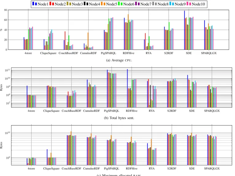
D. Parsimony Share and Parallelize
Figure 3 shows how each cluster node behaves during the Lubm1k query phase and thus provides an idea of how the evaluators allocate resources across the cluster. Such a visualization also confirms some properties one can guess
about evaluators. For example by observing the 4store CPU
average usage in Figure 3a, we can highlight its storage
architecture: the Nodes 6 to 10 are more CPU-active during
the process (about 40% ofCPUwhereas other nodes use about
20%) and thus correspond to the 4store computing nodes while
the other ones (excepting the driver on Node1) correspond to the 4store storing nodes. In addition, the number of bytes sent across the network provides clues to identify the evaluator driver nodes (Figure 3b) i.e. it appears that the Node1 of 4store and RDFHive sends at least 10 times more data than the other nodes (which are receiving). According to several observations made previously (see e.g. Section IV), we know that theRAMusage can be a bottleneck forSPARQLevaluation.
Representing in Figure 3c the maximum allocated RAM per
node during the Lubm1k query phase, we observe that several evaluators are closed to the maximum possible of 16GB per node (see Section III-C): CouchBaseRDF which is an in-memory datastore, CumulusRDF and the three Spark-based
evaluators e.g. S2RDF, SDE and SPARQLGX. On the other
hand, 4store and CliqueSquare need in average less than one order of magnitude than it is possible to allocated while being temporally efficient (see e.g. Section V-A).
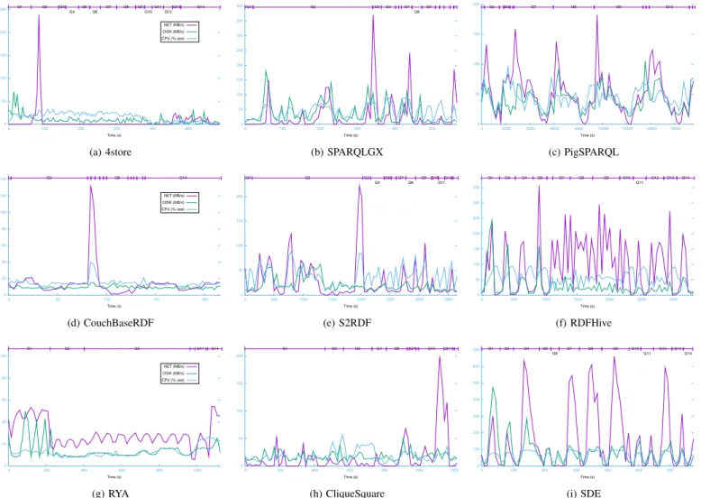
Figure 4 presents resource usages correlated with Lubm1k query evaluation. We give three curves for each evaluator during the Lubm1k query phase: first, the network traffic (sent and received bytes); second, the disk activity (read and write bytes); third, the CPU usage. Moreover, we also divide the time dimension according the needed response times of LUBM queries to observe the resource consumption during one designated query at a glance. We observe that Network and Disk peaks are often synchronous, which means the evaluator reads and transmits or receives and saves data. These correlations are especially observed with the direct evaluators since they have to read at least once the whole dataset to evaluate aSPARQLquery and also have to shuffle intermediate results to join them (see e.g. Figures 4c, 4f & 4i). In addition, we also remark that thanks to their storage models, 4store CliqueSquare or CouchBaseRDF never have to read large amounts of data and we can only observe network peaks when the query has large intermediate results or outputs such as Q14 for example (see e.g. Figures 4a, 4d & 4h).
Paying attention to resource consumption thereby provides information on the real evaluator behaviors. Actually, we found that some systems that dominate in previous features (e.g
SDE for Immediacy) are in fact costly for the cluster in
terms of RAMallocation of CPUaverage usage. Moreover, we
Node1 Node2 Node3 Node4 Node5 Node6 Node7 Node8 Node9 Node10
4store CliqueSquare CouchBaseRDF CumulusRDF PigSPARQL RDFHive RYA S2RDF SDE SPARQLGX 0 20 40 60 80 %
(a) AverageCPU.
4store CliqueSquare CouchBaseRDF CumulusRDF PigSPARQL RDFHive RYA S2RDF SDE SPARQLGX 107 108 109 1010 1011 Bytes
(b) Total bytes sent.
4store CliqueSquare CouchBaseRDF CumulusRDF PigSPARQL RDFHive RYA S2RDF SDE SPARQLGX 109
1010
Bytes
(c) Maximum allocatedRAM.
Fig. 3:CPU, Network andRAM consumptions per node during Lubm1k query phase.
behavior by using as much resources as possible in order to provide an answer as quickly as possible. As a conclusion, if one needs to run concurrent processes while evaluating
SPARQLqueries (e.g. running aSQLservice or data processing
pipelines at the same time), one should rather prefer evaluators whose data storage models are optimized such as 4store or CliqueSquare.
E. Resiliency Having Duplicates
Data Resiliency: When an application processes a very
large dataset stored across many machines, it is interesting for the system to implement some level of tolerance in case a datanode is lost. To implement data resilience, stores typically replicate data across the cluster which implies a larger disk footprint. For our experiments, we stick to the default
replica-tion parameters. As a consequence, the HDFS-based systems
have their data replicated twice and provide some level of data resilience. Table III presents the effective disk footprints (including replication) with Lubm1k and WatDiv1k where the
HDFS-based systems are outlined in gray. Due to their prepro-cessing methods, we note that S2RDF and CliqueSquare need
Systems Lubm1k (GB) WatDiv1k (GB) S2RDF 13.057 15.150 RYA 16.275 11.027 CumulusRDF 20.325 – 4store 20.551 14.390 CouchBaseRDF 37.941 20.559 SPARQLGX 39.057 23.629 CliqueSquare 55.753 90.608 PigSPARQL 72.044 46.797 RDFHive 72.044 46.797 SDE 72.044 46.797
TABLE III: Disk Footprints (including replication).
more disk space to store WatDiv1k than Lubm1k whereas this last one is larger (see Table II). Furthermore, counterintuitively, it appears that evaluators having replicated data can have lighter disk footprints than not-replicated ones e.g S2RDF and RYA versus CouchBaseRDF.
Computation Resiliency: If an application has to eval-uate complex queries (taking e.g. days), it is interesting for the system not to be forced to compute everything from scratch
0 50 100 150 200 250 0 100 200 300 400 500 Q1 Q2 Q3 Q4 Q5 Q6 Q7 Q8 Q9 Q10 Q11 Q12 Q13 Q14 Time (s) NET (MB/s) DISK (MB/s) CPU (% use) (a) 4store 0 50 100 150 200 250 300 350 400 0 100 200 300 400 500 Q1 Q2 Q3 Q4 Q7 Q8 Q9 Time (s) (b) SPARQLGX 0 50 100 150 200 0 2000 4000 6000 8000 10000 12000 14000 16000 Q2 Q4 Q7 Q8 Q9 Q12 Time (s) (c) PigSPARQL 0 20 40 60 80 100 120 140 0 50 100 150 200 Q2 Q8 Q14 Time (s) NET (MB/s) DISK (MB/s) CPU (% use) (d) CouchBaseRDF 0 50 100 150 200 0 500 1000 1500 2000 2500 3000 3500 Q1 Q2 Q3 Q4 Q5 Q7 Q8 Q9 Q10 Q11 Q12 Time (s) (e) S2RDF 0 50 100 150 200 250 300 350 0 500 1000 1500 2000 2500 3000 Q1 Q3 Q4 Q5 Q7 Q8 Q9 Q10 Q11 Q12 Q13 Q14 Time (s) (f) RDFHive 0 20 40 60 80 100 0 200 400 600 800 1000 Q1 Q2 Q3 Q11 Q14 Time (s) NET (MB/s) DISK (MB/s) CPU (% use) (g) RYA 0 50 100 150 200 0 200 400 600 800 1000 1200 Q1 Q2 Q3 Q4 Q5 Q7 Q10 Q11 Time (s) (h) CliqueSquare 0 100 200 300 400 500 600 700 0 100 200 300 400 500 600 Q1 Q3 Q4 Q5 Q6 Q7 Q8 Q9 Q10 Q11 Q12 Q13 Q14 Time (s) (i) SDE
Fig. 4: Resource consumption during Lubm1k query phase.
whenever a machine becomes unreachable. This situation is likely to happen for a variety of reasons (e.g. reboot, failure, network latency). The tested systems exhibit several behaviours when a machine fails during computation. For stores having no data replication, the loss of any machine can stop the computation if the lost data fragment is mandatory; thus some stores fail when a machine is lost: 4store and Cu-mulusRDF; whereas CouchBaseRDF adopts another method waiting seven minutes until the return of the machine. More generally, the HDFS-based triplestores cannot lose mandatory
fragments of data, thereby RDFHive, SPARQLGX,SDE, RYA,
and CliqueSquare still succeed when one (or even two) ma-chine fails during computation; however, PigSPARQL waits indefinitely the return of the lost partition. For stores having a master/slave structure e.g. SPARQLGX, the loss of the node hosting the master process prevents any result to be obtained. From our tests, only two different methods successfully faced a loss of worker nodes: (1) waiting for their returns e.g. CouchBaseRDF and PigSPARQL; (2) using the remaining nodes and benefiting from data replication e.g. CliqueSquare,
RDFHive, RYA, S2RDF, SDE,SPARQLGX.
F. Summary At a glance
Figure 5 presents a Kiviat chart in which the tested systems are ranked, based on Lubm1k and WatDiv1k according to all the features already discussed in Section V. More particularly, evaluator ranks on the two “velocity” axes (one for Lubm1k and one for WatDiv1k) are based on average response time considering only successful queries. This representation gives at a glance clues to select an evaluator. For instance it appears that 4store is especially relevant when velocity and parsimony are important and less importance is given to resiliency.
SDE also appears as a reasonnable choice when all criteria
(including its potential cost on a cloud platform) but parsimony matter.
VI. RELATEDWORK
This study benefited from the extensive earlier works on
benchmarks for RDF systems. There are many benchmarks
designed for evaluating RDF systems [18]–[25]. Some of
them are particularly popular: LUBM [19], WatDiv [20],
SP2Bench [25], DBpedia Bench [23], BSBM [24], and
Velocity Lubm1k Velocity WatDiv1k Immediacy Parsimony Dynamicity Resiliency 4store CliqueSquare CouchBaseRDF CumulusRDF PigSPARQL RDFHive RYA S2RDF SDE SPARQLGX
Fig. 5: System Ranking (farthest is better).
for testing the BGP fragment, and because we wanted deter-ministic data generators for ensuring reproducibility of our results. Compared to all these works, we focus on testing distribution techniques by considering a set of 10 state-of-the-art implementations; see e.g. [3], [14], [26] for recent surveys about distributedRDFdatastores and their storage approaches. Compared to studies included in the aforementioned bench-marks, we consider more competing implementations on a
common ground. Furthermore, while earlier works on RDF
benchmarks exclusively focused on measuring elapsed times (and sometimes disk footprints), we measure a broader set of indicators encompassing e.g. network usage. This allows to refine the comparative analysis according to features and requirements from a slightly higher perspective, as discussed in Section V. This also allows to more precisely identify the bottlenecks of each system when they are pushed to the limits. Finally, this work was inspired by the empirical study car-ried out by Cudr´e et al. where five distributed RDFdatastores using various NoSQL backends were evaluated [9]. Our work does not invalidate earlier results but supplement them with more results. In particular, in the present work, we update the list of evaluators (we consider more of them, with more recent ones) and we also focus on ranking the candidates depending on various features thanks to the broader set of metrics we analysed.
VII. CONCLUSION
We conducted an empirical evaluation of 10
state-of-the-art distributed SPARQL evaluators on a common basis. By
considering a full set of metrics, we improve on traditional empirical studies which usually focus exclusively on temporal considerations. We proposed five new dimensions of com-parison that help in clarifying the limitations and advantages
of SPARQL evaluators according to use cases with different
requirements.
REFERENCES
[1] P. Hayes and B. McBride, “RDF semantics,” W3C Rec., 2004.
[2] “SPARQL 1.1 overview,” March 2013,
http://www.w3.org/TR/sparql11-overview/.
[3] Z. Kaoudi and I. Manolescu, “RDF in the clouds: a survey,” The VLDB
Journal, vol. 24, no. 1, pp. 67–91, 2015.
[4] J. Dean and S. Ghemawat, “Mapreduce: simplified data processing on
large clusters,” Communications of the ACM, vol. 51, no. 1, pp. 107– 113, 2008.
[5] M. Zaharia, M. Chowdhury, T. Das, A. Dave, J. Ma, M. McCauley,
M. J. Franklin, S. Shenker, and I. Stoica, “Resilient distributed datasets: A fault-tolerant abstraction for in-memory cluster computing,” NSDI, 2012.
[6] C. Olston, B. Reed, U. Srivastava, R. Kumar, and A. Tomkins, “Pig
latin: a not-so-foreign language for data processing,” in SIGMOD. ACM, 2008, pp. 1099–1110.
[7] S. Harris, N. Lamb, and N. Shadbolt, “4store: The design and
imple-mentation of a clustered RDF store,” SSWS, 2009.
[8] A. Sch¨atzle, M. Przyjaciel-Zablocki, S. Skilevic, and G. Lausen,
“S2RDF: RDF querying with SPARQL on spark,” VLDB, pp. 804–815, 2016.
[9] P. Cudr´e-Mauroux, I. Enchev, S. Fundatureanu, P. Groth, A. Haque,
A. Harth, F. L. Keppmann, D. Miranker, J. F. Sequeda, and M. Wylot, “NoSQL databases for RDF: An empirical evaluation,” ISWC, pp. 310– 325, 2013.
[10] Abadi, Marcus, Madden, and Hollenbach, “Scalable semantic web data
management using vertical partitioning,” VLDB, 2007.
[11] R. Punnoose, A. Crainiceanu, and D. Rapp, “RYA: a scalable RDF triple
store for the clouds,” in International Workshop on Cloud Intelligence. ACM, 2012, p. 4.
[12] K. Shvachko, H. Kuang, S. Radia, and R. Chansler, “The hadoop
distributed file system,” in Mass Storage Systems and Technologies
(MSST), 2010 IEEE 26th Symposium on. IEEE, 2010, pp. 1–10.
[13] F. Goasdou´e, Z. Kaoudi, I. Manolescu, J.-A. Quian´e-Ruiz, and S.
Zam-petakis, “Cliquesquare: Flat plans for massively parallel RDF queries,”
in ICDE. IEEE, 2015, pp. 771–782.
[14] D. C. Faye, O. Cur´e, and G. Blin, “A survey of RDF storage
ap-proaches,” Arima Journal, vol. 15, pp. 11–35, 2012.
[15] G. Ladwig and A. Harth, “CumulusRDF: linked data management on
nested key-value stores,” SSWS 2011, p. 30, 2011.
[16] D. Graux, L. Jachiet, P. Genev`es, and N. Laya¨ıda, “SPARQLGX:
Ef-ficient Distributed Evaluation of SPARQL with Apache Spark,” ISWC, 2016.
[17] A. Sch¨atzle, M. Przyjaciel-Zablocki, and G. Lausen, “PigSPARQL:
Mapping SPARQL to pig latin,” in Proceedings of the International
Workshop on Semantic Web Information Management. ACM, 2011,
p. 4.
[18] S. Qiao and Z. M. ¨Ozsoyo˘glu, “Rbench: Application-specific RDF
benchmarking,” in SIGMOD. ACM, 2015, pp. 1825–1838.
[19] Y. Guo, Z. Pan, and J. Heflin, “LUBM: A benchmark for OWL
knowledge base systems,” Web Semantics, 2005.
[20] G. Aluc¸, O. Hartig, M. T. ¨Ozsu, and K. Daudjee, “Diversified stress
testing of RDF data management systems,” in ISWC. Springer, 2014,
pp. 197–212.
[21] R. Angles, P. Boncz, J. Larriba-Pey, I. Fundulaki, T. Neumann, O.
Er-ling, P. Neubauer, N. Martinez-Bazan, V. Kotsev, and I. Toma, “The linked data benchmark council: a graph and RDF industry benchmark-ing effort,” ACM SIGMOD Record, vol. 43, no. 1, pp. 27–31, 2014.
[22] G. Demartini, I. Enchev, M. Wylot, J. Gapany, and P. Cudr´e-Mauroux,
“Bowlognabench – Benchmarking RDF Analytics,” in International Symposium on Data-Driven Process Discovery and Analysis. Springer, 2011, pp. 82–102.
[23] M. Morsey, J. Lehmann, S. Auer, and A.-C. N. Ngomo, “DBpedia
SPARQL Benchmark – Performance assessment with real queries on real data,” ISWC, pp. 454–469, 2011.
[24] C. Bizer and A. Schultz, “The berlin SPARQL benchmark,” IJSWIS,
2009.
[25] M. Schmidt, T. Hornung, G. Lausen, and C. Pinkel, “SP2Bench: a
SPARQL performance benchmark,” ICDE, pp. 222–233, 2009.
[26] G. A. Atemezing and F. Amardeilh, “Benchmarking commercial rdf
stores with publications office dataset,” in European Semantic Web