Potential impacts of changing agricultural activities on scenic beauty - a prototypical technique for automated rapid assessment

Potential impacts of changing agricultural activities on scenic beauty – a

prototypical technique for automated rapid assessment

Marcel Hunziker

and Felix Kienast

Swiss Federal Institute of Forest, Snow and Landscape Research, Department of Landscape Ecology, 8903 Bir-mensdorf, Switzerland; ∗Corresponding author: tel.: +41/1/739 24 59, fax +41/1/737 40 80, E-mail: marcel.hunziker@wsl.ch, http://www.wsl.ch/land/evolution/evolution.html)

Received 6 September 1996; Revised 24 February 1998; Accepted 16 May 1998

Key words: landscape; agriculture; land abandonment; reforestation; aesthetics; landscape preference; social science; image experiments; pattern analysis; GIS

Abstract

As a result of the liberalisation of the agricultural market, mountain regions in Central Europe are at great risk of experiencing increasing land abandonment and spontaneous reforestation. Prior to taking measures for land-scape maintenance, the ecological and landland-scape-aesthetic consequences of land abandonment should be analysed. This paper addresses the aesthetic component of such analyses: we investigated whether lay people perceive land abandonment and spontaneous reforestation as a loss or a gain and developed a prototypical technique for rapid aesthetic assessment of reforestation scenarios for vast regions.

First, we conducted image experiments to assess the respondents’ reactions to increasing levels of reforestation. Based on these experiments we concluded that a medium degree of reforestation is most desirable. Second, we analysed the relationship between scenic beauty and landscape patterns and found that landscape preference values correlate significantly with various quantitative measures of the landscape pattern (e.g., diversity and contagion indices of grey-tone and colour images). Third, we applied a GIS-assisted ‘moving-window’ technique to trans-form spatially explicit remote-sensing data (in particular orthophotos) of a test region to spatially explicit data of landscape-pattern indices. Thanks to the significant positive correlation between pattern indices and landscape preference values, the resulting maps can preliminarily be interpreted as ‘beauty’-maps of the test-region.

Introduction

The overall aim of landscape conservation concepts is to maintain or even improve the physical quality and the scenic beauty of landscapes (Hollenhorst et al. 1993; Kangas et al. 1993; Haider, 1994; Ribe 1994; Peccol et al. 1996). The latter is important because the general public’s gain from conservation efforts is primarily an aesthetic one (Anwander et al. 1990; Daniel and Boster 1976; Hoisl et al. 1987; Nassauer 1989, 1992; Nohl 1982, 1988). To inhibit undesirable negative effects of land use on landscape qualities or to initiate positive developments with appropriate in-centives, scenario evaluation – commonly based on landscape models – is a must for landscape planners (Baker 1996; Flamm and Turner 1994; Gardner et al.

1987; Liu 1993; Turner et al. 1993, 1994; Schippers et al. 1996).

A likely development – at least for Central Europe – is the intensification of agricultural production on highly productive land and, at the same time, land abandonment – followed by spontaneous reforestation – on land with a low production potential. This land use segregation in the agricultural sector is primar-ily attributable to the liberalisation of the agricultural market (Anwander et al. 1990; Hunziker 1995; Pinto-Correia et al. in press). Modern landscape conserva-tion schemes that include both the ecological and the landscape-aesthetics perspective draw a multifaceted picture of the impacts of intensification and abandon-ment on landscape qualities: Agricultural intensifica-tion is valued negatively from both an ecological and

a landscape-aesthetics perspective, because of result-ing soil degradation and a loss of traditional landscape components (Hoisl et al. 1989; Nassauer 1992; Nohl 1982, 1988; Raba 1997). In the case of land aban-donment, the ecological and the landscape-aesthetics perspective yield ambiguous assessments:

• From the ecological point of view, the

abandon-ment of land and subsequent reforestation is a gain in terms of a lowered input of pesticides and fer-tilisers. However, the concurrent loss of the patchy land mosaic is often linked with a loss of biodi-versity (Burel and Baudry 1995; Dale et al. 1994; Naiman et al. 1993; Ruzicka 1993).

• From the landscape-aesthetics point of view, it can

be assumed that partially reforested landscapes are what most people prefer visually; completely over-grown areas, however, are likely to receive lower preference. Hunziker (1995) discusses the theoret-ical legitimisation of this assumption with the aid of the empirical findings and models of Bourassa (1991), Kaplan et al. (1989), Lamb and Purcell (1990), Purcell (1987) and Schroeder (1986), as well as his own research findings gleaned from focused interviews.

Since the processes of intensification and abandon-ment are important forces driving Central Europe’s landscape change, the issue is of great concern for landscape planning agencies, which are confronted with the problem that for each affected region, sce-narios have to be generated and evaluated on the basis of ecological and aesthetics schemes. Based on the re-sults of these evaluations the optimum scenario may be chosen and worked for with appropriate incentives. Taking into account the vast areas of land that might be abandoned in Europe during the next decades, land managers need rapid, simple assessment procedures for evaluating these scenarios.

However, none of the landscape-aesthetics ap-proaches found in the literature seems to satisfy fully the requirements of the planners, who need empiri-cally based procedures that are simple and rapid, and suited for larger regions. The major existing methods are documented in Bishop and Hulse (1994), Brown (1994), Daniel and Boster (1976), Kaplan (1979), Shafer et al. (1969) and Steinitz (1990). In all these approaches, scenic beauty is predicted based on re-gression models. The explanatory variables are de-scriptive, ‘objective’ criteria of the landscape. These approaches would be most appropriate for rapidly as-sessing scenarios of vast regions, if the descriptors of landscape could be directly, automatically, and

objec-tively generated from spatially explicit data such as aerial photographs, satellite images, or digitised maps. However this is not the case:

• Brown (1994), Daniel and Boster (1976), Kaplan

(1979) as well as Steinitz (1990) estimate the ex-planatory variables of the regression models on the basis of expert knowledge: all images that are evaluated by the respondents are screened by the authors for ‘objectively’ determined landscape criteria. This procedure has the disadvantage that both the parameter scenic beauty and the ‘objec-tively’ determined landscape measures are valued subjectively, a shortcoming that is criticised by Steinitz (1990).

• Shafer et al. (1969) propose a method that solves

the shortcoming of subjectively measured image descriptors: here scenic beauty is predicted on the basis of abundance ratios of various landscape elements on photographs. However, performing this assessment on aerial photographs is time con-suming and expensive since it requires a detailed, thematic mapping of landscape elements. The requirement of rapidity is therefore not fulfilled.

• The procedure of Bishop and Hulse (1994) meets

the requirement of rapidity, but only if de-tailed digitised land-use data are easily accessible. Scenic beauty is predicted on the basis of spatially explicit predictors (land-use categories) stored in a GIS. An application of this method for larger regions requires detailed thematic maps of vari-ous land-use categories, a usually time-consuming investment for planning agencies.

Since none of the approaches listed above was found to satisfy fully the needs of the planners, we aimed our efforts at developing a new assessment tech-nique. The technique builds upon the basic philosophy of the existing approaches, particularly on regressing scenic beauty with ‘objective’ landscape descriptors, in our case even objectively measured formal land-scape criteria. The exclusive use of formal criteria can be justified since agricultural changes, in particular spontaneous reforestation, primarily affect the formal content of a landscape (i.e., the landscape pattern). Our assessment technique shall be based upon:

(1) an empirical relationship between the changing formal content of landscape and scenic beauty, i.e., we had to gain empirical knowledge about the influence of spontaneous reforestation on scenic beauty;

(2) easily and objectively measured formal landscape criteria; we had to find a mathematical index that

is (a) sensitive to the changes in landscape pattern caused by spontaneous reforestation (b) a good predictor for scenic beauty, and (c) suitable for use in aerial photographs.

Methods

Image experiments for investigating the influence of spontaneous reforestation on scenic beauty

Respondents

As this project was largely concerned with developing and testing a prototypical technique for rapidly assess-ing the effect of landscape changes on the aesthetic value, we restricted our analysis to easily accessible persons – in our case 181 university students from various disciplines. To further the development of our technique as well as to plan for real planning-applications, the empirical base would have to be enlarged and a representative sample of people living in Europe would have to be interviewed.

Images

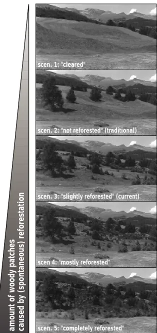
The respondents were shown images representing sce-narios of different stages of spontaneous reforestation. Because of the large number of respondents required, it was not feasible to provide a real landscape expe-rience. Therefore, coloured images had to be used instead, a common practice in scenic beauty estima-tion approaches (e.g. Daniel and Boster 1976; Kaplan et al. 1972; Shafer et al. 1969; Zube 1973). Since we intended to compare different stages of reforestation and not different landscape types, we decided to use images of one landscape type in different stages of re-forestation. Unfortunately, a suitable and qualitatively satisfactory series of historical photos showing the reforestation of a single location was not available. Ar-tificially creating such a series by using photographs of different locations would have the disadvantage that the respondents might be biased by variables other than reforestation, for example the changing back-grounds of the different photographs (Hunziker 1992). Thus, we generated a series of ‘reforestation images’ (Figure 1) by subjecting one single, real photograph of a landscape to computer-aided photo editing. Numer-ous scientific studies have demonstrated the validity of performing experiments using photographs in general, as well as using simulated material (e.g., Bishop and Leahy 1989; Daniel and Boster 1976; Jarvis 1990; Nohl 1974; Oh 1994; Stamps 1997). To develop the

scen. 1: "cleared"

scen. 2: "not reforested" (traditional)

scen. 3: "slightly reforested" (current)

scen 4: "mostly reforested"

scen. 5: "completely reforested"

amount of woody patches

caused by (spontaneous) reforestation

Figure 1. The landscape scenarios used in the image experiments.

technique further, it would be desirable to use more than one scene.

Seven images were used in this study. The number was kept small to allow various forms of assessment without requiring too much of each respondent’s time. Five of the seven images show the selected scene un-der different reforestation scenarios (Figure 1). The scenario 1, labelled ‘cleared’, is fairly hypothetical but is probably the only one that would allow farmers to run an economically profitable enterprise without subsidies. The scenario 2, labelled ‘not reforested’,

all random sampling

group 1 group 2

pair comparison scoring

• investigate the influence of spontaneous reforestation on scenic beauty

• test the influence of methods on results e x p e r i m e n t 1 respondents: procedure: analysis: purpose: • descriptive statistics • correlation analysis

test the influence of image quality on results e x p e r i m e n t 2

respondents:

procedure:

analysis: purpose:

two sample t-test of the polarity profiles of the two images image-assessment all random sampling group 1 group 2 coloured photos semantic differentials with b/w-raster prints

test the influence of image manipulation on results e x p e r i m e n t 3 respondents: procedure: analysis: purpose: descriptive statistics all

find out the original, "real" image and indicate difficulty as well as reasons of the choice

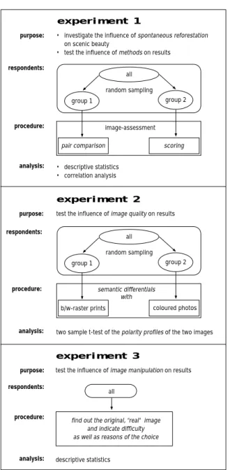
Figure 2. The design of the image experiments conducted.

shows the ‘traditional’ condition of the land in the 1950s, whereas the other scenarios – including sce-nario 3, which shows the current condition – depict stages of reforestation as documented in succession analyses (Raba 1997). We have chosen to present here results of respondents’ reactions to these five images only. In the experimental runs, however, two further images were included that show elements of human settlement. This landscape variable was added to pre-vent respondents from recognising the reforestation sequence too easily.

Procedures

We performed three experiments to find out people’s response to spontaneous reforestation and to control disturbance variables. Figure 2 gives an overview of the purpose of each of the three experiments and the methods used to carry out each one.

• The first experiment was designed to test the

as-sumption that a landscape receives highest prefer-ence when there is a medium level of spontaneous reforestation. The images discussed in the section ‘Images’ were shown in the form of slides. The re-spondents assessed these images according to the integral criterion ‘preference’. Out of numerous possible assessment techniques we selected pair comparison and scoring (Friedrichs 1985; Stamps 1997).

The respondents were randomly separated into two groups. Each group carried out one of the two pro-cedures. This experimental set-up allowed us to cross-check the results of the two procedures and to evaluate a potential bias of the methods. The chance of a bias was low, as shown by Schroeder (1984) Stamps (1997) or Zube et al. (1974). In the pair comparison, (Friedrichs 1985), each im-age was compared with all the others. For each of the 21 comparisons, one image had to be selected as preferable. In the scoring procedure, which is closely related to the technique used by Daniel and Boster (1976), the seven images were shown to the respondents three times, one after another and in random order to avoid a ranking according to in-creased reforestation. In the first assessment, each image was shown for 2 s, in the second run for 10 s, and in the third run for 5 s. Scores ranging from 1 (‘strong dislike’) to 6 (‘strong like’) had to be given during the second viewing and could be cor-rected during the final viewing. This experimental design was chosen in order to allow comparison of the different images during the viewing ses-sion. Thus, consistency of the judgements could be increased.

• The second experiment was designed to

investi-gate the influence of image quality on the assess-ment of a landscape (Oh 1994; Stamps 1997). This check was necessary since in the course of this project (and probably in later practical applica-tions) aerial photographs of much lower quality and in black and white were used. Thus, some re-spondents had to asses a colour image of one of the landscape states, whereas a control group assessed a black-and-white raster print of the same

land-scape state. A semantic differential was applied (Osgood 1952). This process involves mapping emotional reactions to a stimulus (in our case, the evaluation of a landscape) according to a number of contrasting characteristics. To this end, respon-dents were given a list consisting of contrasting pairs of adjectives and marked a bipolar scale from 1 to 7 for each pair. The analysis of the resulting polarity profiles would reveal whether any dif-ferences in assessment could be attributed to the image quality only.

• In the third experiment, we further checked the

va-lidity of our photo assessment by testing whether the assessment of landscapes is significantly al-tered by the use of manipulated images instead of real photographs. We investigated whether the manipulated images could be recognised as such because of technical effects, and whether recogni-tion of the true condirecogni-tion of the landscape would influence the assessments. To determine this, the respondents were shown all the images once again after the image assessment procedure. This time, however, the images were shown simultaneously (reduced onto two slides), and respondents were requested to find out the ‘real’ one. Furthermore they were asked to assess the difficulty of the selection process and give reasons for their choice. To analyse the responses we used both univari-ate and multivariunivari-ate statistical methods, in particular MANOVA. Commercial software packages such as Excel, Statview, Datadesk and Systat were applied. Pattern analysis of the terrestrial photographs To determine whether human preference for land-scapes (i.e., landscape images) correlates with the formal content (patterns of the images), we subjected the photographs used in the experiments to quantita-tive pattern analysis. The resulting indices were then correlated with the corresponding preference ratings of the respondents.

There have been numerous attempts to describe landscape patterns quantitatively using indices de-rived from information theory and fractal geometry (Gustafson and Parker 1992; Hulshoff 1995; Li and Reynolds 1993; McGarigal and Marks 1994; O’Neill et al. 1992; Plotnick et al. 1993; Qi and Wu 1996; Schumaker 1996; Turner 1990; Turner et al. 1994a, 1994b). In the present study, both black-and-white, and colour images of landscapes were analysed. The classes here were not, however, distinguished on the

basis of landscape elements, as would be usual in landscape-ecological pattern analysis, but rather ac-cording to grey scales or colour schemes. Thus, the quantitative landscape measures do not evaluate the complexity of elements, but of unclassified landscape patterns in the form of grey tones or colours.

For the pattern analyses we used the following colour schemes and grey scales: 2 and 10 grey tones, as well as 12, 16, 20, and 32 colours. Image resolu-tion was either 36 dots per inch (dpi) or 72 dpi. The purpose of varying image quality was to identify the index and the image quality that are most suitable for use in predicting scenic beauty.

McGarigal and Marks’ computer program (1994) was used to calculate the index values of the im-ages. Calculations were performed at the landscape level (i.e., for the entire image, including the sky. The latter was identical in all images, thus its in-fluence on the indices was constant). The following pattern indices were considered for calculation: con-tagion, double-log fractal dimension, interspersion, mean nearest-neighbour distance nearest-neighbour standard deviation, nearest-neighbour coefficient of variation, number of patches, patch density, mean patch size, patch size standard deviation, total edge, Simpson’s, and modified Simpson’s and Shannon’s diversity and evenness index. For all formulae see McGarigal and Marks (1994).

The meaning of the indices

Note that all indices calculated in the course of this project refer to homogeneous grey tone or colour patches and not to formal landscape elements. The simple indices ‘number of patches’ and ‘patch density’ usually are best considered as representing the config-uration of the image, even though they are not spatially explicit, (i.e., they are independent of the location of the patches on the photograph). Others, such as con-tagion or eveness, describe the spatial distribution of grey or coloured patches. Contagion is calculated ac-cording to the formula suggested by Li and Reynolds (1993). This formula calculates the probability that two randomly chosen adjacent cells belong to two different patch types. Contagion measures the extent to which patch types are aggregated. High conta-gion values mostly occur in images with few large, contiguous patches (low complexity), whereas low values generally characterise images with many small, dispersed patches (high complexity). Unlike the con-tagion index, which is based on cell adjacencies, the interspersion index measures patch adjacencies, or in

other words, each patch is evaluated for adjacency with all other patch types. Internal cells of the patch are ignored. Thus, images with higher values are those in which patches of the same type are homogeneously distributed throughout the image (i.e., equally adja-cent to each other), whereas images of lower values are those in which patches of the same type are not homogeneously distributed. The diversity and even-ness quantify patch composition of the images. For a detailed discussion of the parameters, see McGari-gal and Marks (1994). We used both Simpson’s and Shannon’s diversity index, as well as Simpson’s and Shannon’s evenness index. Simpson’s diversity index is less sensitive to the presence of rare types and has an interpretation that is much more intuitive than that of Shannon. Simpson’s diversity index (Simpson 1949) measures the probability that any patches selected at random would be of different types. The higher the values, the greater the probability that two randomly selected patches would be different (high complexity). The evenness indices measure the distribution of area among patch types. It is expressed as the observed level of diversity divided by the maximum possible diversity for that given number of patch types. Since it measures to what degree the distribution of area among patch types is even ‘0’ indicates that only one patch dominates the scene (low complexity), and ‘1’ indicates that all patch types are evenly distributed. The ‘moving-window’ technique for aesthetically assessing photographs of whole regions

The landscape images evaluated by our respondents represent an excerpt from the whole expanse of a re-gion. Such a mesoscale excerpt roughly corresponds to a person’s momentary field of vision (i.e., the excerpt of the landscape a person can see at once without any eye movement). However, as mentioned previously, landscape planning relies on information about whole regions. This means that it is necessary to extrapolate from the data on the mesoscale (the level of a person’s momentary field of vision) to the macroscale (the level providing an overview of a whole region – a map). For our purpose the GIS-assisted ‘moving-window’ technique seemed the most suitable way to perform the spatial extrapolations. Accordingly, a window de-fined to correspond to the mesoscale image excerpt was passed over grey-tone images of the whole ex-panse of a test-region (macroscale) where spontaneous reforestation already occurs (Lower Engadin, Central Alps, Switzerland). Output values at each cell of a grid

placed over the image was the ‘beauty’ index for the specified mesoscale neighbourhood of the cell. This technique simulates an artificial – yet closely real – viewer walking across the landscape with one given angle of the viewing perspective and with a given field of vision. In a first step, we selected an angle of the viewing perspective that corresponds to a terrestrial grey-tone photograph taken from the opposite side of the valley.

Such terrestrial overview images are not very useful for landscape planners because implementing planning measures means locating perimeters on or-thogonal maps and plans. In our case, the terrestrial views would have to be orthogonalised which would require a great deal of effort. The result, however, would not be satisfactory since hidden areas would be blank in the orthogonal image. Thus, in a sec-ond trial we applied the moving window technique to orthophotos. For each cell we calculated the ‘scenic beauty index’ and generated a map of scenic beauty that can be used for planning purposes. This proce-dure simulates the view of an artificial – non-real – viewer who observes the landscape at a vertical an-gle (i.e., the only difference to the terrestrial photos is the angle of the viewing perspective). By doing so, areas that are usually hidden in terrestrial photographs become visible, leading to an overestimation of the diversity indices and, therefore, to an overestimation of the scenic beauty value. Thus, the obtained values can be considered as maximum values. Since we are mainly interested in comparing scenarios of the same landscape, this deficiency is compensated for by the advantage that the assessment is mostly independent of the viewing perspective of the observer.

Results

The influence of spontaneous reforestation on scenic beauty

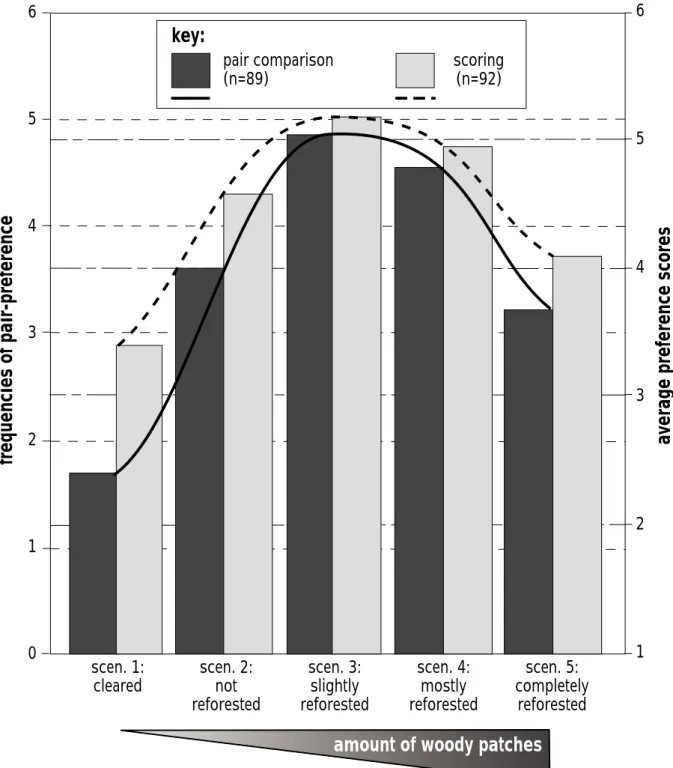
As shown in Figure 3, the curves representing pref-erence values given for increasing degrees of refor-estation are similar to a bell, with a peak at the level of partial reforestation. Furthermore, the prefer-ence values for the different images are for the most part significantly different for all possible pairs and both procedures (two sample t-test, significance level

p= 0.05. The only non-significant difference

con-cerns the scores for scenario 3 vs scenario 4. A land-scape with a medium level of reforestation seems to be

scen. 2:

not

reforested

scen. 3:

slightly

reforested

scen. 4:

mostly

reforested

scen. 5:

completely

reforested

scen. 1:

cleared

6

1

2

3

4

5

6

5

4

3

2

1

0

pair comparison

(n=89)

key:

scoring

(n=92)

average preference scores

frequencies of pair-preference

amount of woody patches

Figure 3. Preference values (resulting from two photo assessment procedures) for the scenarios of different stages of spontaneous reforestation

the type of landscape people find most attractive. This result, therefore, substantiates the assumption arising from existing theories and prior research (Hunziker 1995).

As described in the section ‘Methods’, the land-scapes were evaluated by two comparable groups us-ing two different procedures, namely pair comparison and scoring. Figure 3 shows that the two proce-dures resulted in rather similar ‘preference curves.’ The visual interpretation indicates only one difference, namely, that the preference values for the extreme conditions scenario 1 (’cleared’) and scenario 5 (‘com-pletely reforested’) were assessed more moderately (i.e., less negatively) in the scoring procedure than in the pair comparison method. This can be explained in part by the subjects’ reluctance in the scoring method to give very low scores (1 or 2). When comparing image-pairs, however, the respondents were unaware of the fact that (almost) never selecting an image as preferable was equivalent to giving it a very low score. This difference notwithstanding, the procedures pro-duced very similar results, i.e., if the ranking order alone is considered, then the results were identical (Spearman rank correlation coefficient= 1.00).

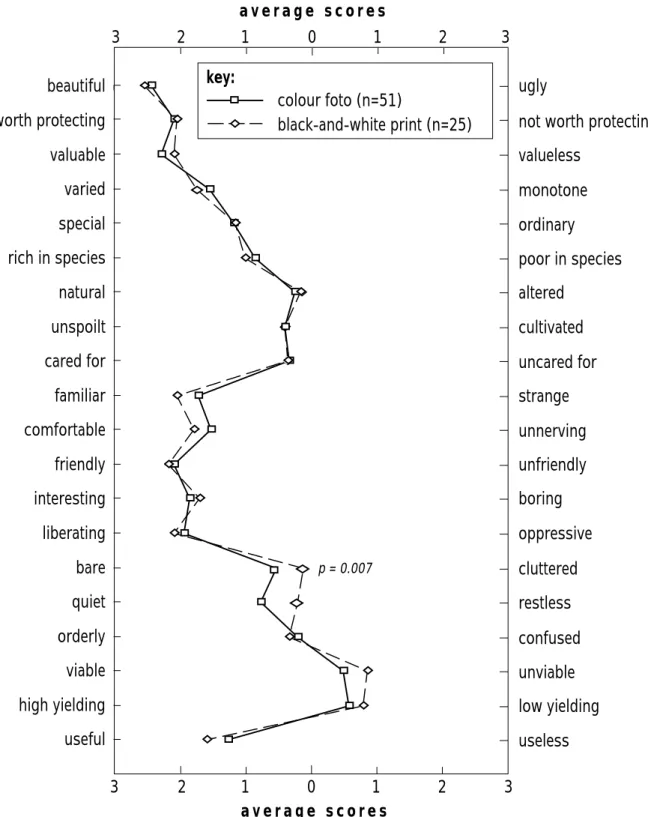
Visual comparison of the two polarity profiles (Figure 4) shows two almost identical profiles for the assessments of both the black-and-white raster print and the colour photograph. The statistical analysis (two-sample t-tests), as well, showed that only the word pair ‘bare’/‘cluttered’ was assessed significantly differently (p= 0.007). Apart from this, the quality of the image did not seem to influence subjects’ assess-ments, even when the differences between the image qualities were very large.

Although 43% percent of the subjects managed to recognise the real image, they also admitted that identifying it was ‘very difficult’ or ‘difficult’ (90%). In their replies to the open question, ‘How did you find out the photograph depicting the actual landscape condition?’, almost all the respondents indicated that it had to do with the contents of the landscape and what they expected a landscape today to look like. The image quality was almost never mentioned as a factor in identifying the real image. There also were no sig-nificant differences in the assessments of the images by those who succeeded in identifying the real image correctly and those who picked the wrong one. This suggests that we can, for the time being, assume that the validity of photo assessments is not affected by the use of simulated material.

The relationship between scenic beauty and landscape patterns

To evaluate the statistical correlation between scenic beauty and landscape patterns we calculated the Spear-man rank correlation coefficients between the pat-tern indices and the preference values of each image (Table 1).

Correlation coefficients between the preference values and the individual indices differed widely. The measures for interspersion/juxtaposition, evenness and diversity correlated best. The explained variance, how-ever, is not higher than 36% (r2). For the explanatory variables fractal dimension, total edge and neighbour-hood measures, we found the highest numbers of non-significant correlations. We conclude, therefore, that diversity, evenness and interspersion/juxtaposition are the most convenient indices to express scenic beauty in an assessment of spontaneous reforestation. Diver-sity, as the most common index, is suggested to have priority.

It is evident from Table 1 that the images with a relatively high degree of generalisation of the grey or colour scales (10 grey tones; 12 colours) correlated best. The more detailed the images, the lower the cor-relation was found to be. This was most likely because patches with the same identification in terms of grey scale become more and more isolated in the high res-olution images and no longer exhibit what could be called a relevant unit for viewing. Thus, the assess-ment should be performed on images with a relatively low resolution (e.g., 36 dpi), where the correlation be-tween the index values and the preference values is strongest. In a further development of the technique an index or an index-combination should be found that can be used to explain more than 36% of the variance (see ‘Discussion’ section for further details).

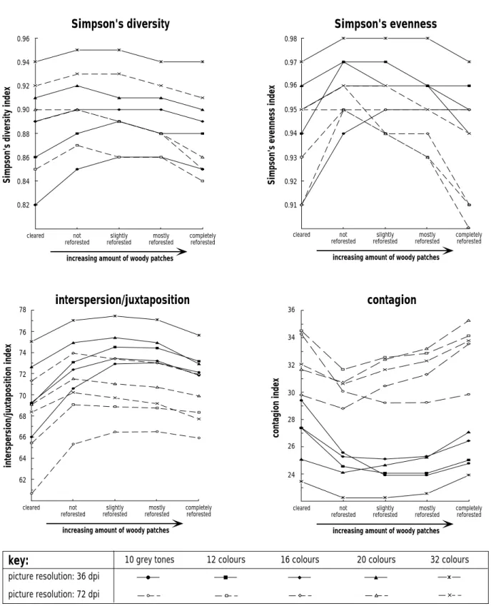
The four indices highlighted in Table 1 are fur-ther evaluated in Figure 5. Interspersion/juxtaposition, evenness and diversity correlated positively with re-spondents’ ratings, resulting in hill-shaped curves for the index values. Contagion appeared to correlate neg-atively with the preference rating, hence the U-shaped curves.

A prototypical map of scenic beauty

Having shown that people’s preferences correlate with quantitative measures of landscape pattern, we un-dertook a spatial extrapolation using the ‘moving-window’ technique described in the ‘Methods’ sec-tion. All macroscale images were subjected to this

3

2

1

0

1

2

3

3

2

1

0

1

2

3

beautiful

worth protecting

valuable

varied

special

rich in species

unspoilt

cared for

familiar

comfortable

friendly

interesting

liberating

bare

quiet

orderly

viable

high yielding

useful

colour foto (n=51)

black-and-white print (n=25)

key:

ugly

not worth protecting

valueless

monotone

ordinary

poor in species

altered

cultivated

uncared for

strange

unnerving

unfriendly

boring

oppressive

cluttered

restless

confused

unviable

low yielding

useless

natural

a v e r a g e s c o r e s

a v e r a g e s c o r e s

Figure 4. Polarity profiles referring to different image qualities of the same image: The colour photograph had an unknown, but very fine grain

62 64 66 68 70 72 74 76 78 interspersion/juxtaposition index 0.82 0.84 0.86 0.88 0.90 0.92 0.94 0.96

Simpson's diversity index

contagion index 24 26 28 30 32 34 36

Simpson's evenness index

0.91 0.92 0.93 0.94 0.95 0.96 0.97 0.98

10 grey tones 12 colours 16 colours 20 colours 32 colours

key:

picture resolution: 36 dpi picture resolution: 72 dpi

Simpson's diversity

Simpson's evenness

contagion

interspersion/juxtaposition

increasing amount of woody patches not reforested slightly reforested mostly reforested completely reforested cleared

increasing amount of woody patches not reforested slightly reforested mostly reforested completely reforested cleared

increasing amount of woody patches not reforested slightly reforested mostly reforested completely reforested cleared

increasing amount of woody patches not reforested slightly reforested mostly reforested completely reforested cleared

Figure 5. Selected quantitative landscape measures for the five images exhibiting scenarios of different stages of spontaneous reforestation

171

Landscape index Correlation coefficients between the preference values and the values of the landscape pattern indices Image resolution (dots per inch, dpi) and number of grey tones (gt) or colours (c)

36 dpi/10 gt 36 dpi/12 c 36 dpi/16 c 36 dpi/20 c 36 dpi/32 c 72 dpi/10 gt 72 dpi/12 c 72 dpi/16 c 72 dpi/20 c 72 dpi/32 c

Number of patches +0.38 +0.28 +0.28 +0.60 +0.56 +0.52 +0.18 +0.34 +0.43 +0.43

Patch density +0.38 +0.28 +0.28 +0.60 +0.56 +0.52 +0.18 +0.34 +0.43 +0.43

Mean patch size −0.17 ns +0.51 +0.51 +0.51 ns ns +0.51 ns +0.51

Patch size standard deviation ns −0.54 −0.39 −0.38 +0.59 −0.37 −0.28 +0.28 +0.28 −0.27

Total edge +0.38 +0.28 +0.28 −0.21 ns +0.28 +0.43 ns ns +0.14

Double log fractal dimension ns ns +0.51 ns ns +0.59 +0.17 +0.51 +0.51 +0.51

Mean nearest neighbor ns ns ns +0.19 ns nc nc nc nc nc

Nearest neighbor standard deviation ns −0.25 −0.22 −0.25 −0.20 nc nc nc nc nc

Nearest neighbor coefficient of variation ns −0.12 −0.22 −0.51 ns nc nc nc nc nc

Shannon’s diversity index +0.56 +0.59 +0.43 +0.34 +0.34 +0.56 +0.43 ns ns +0.27

Simpson’s diversity index +0.61 +0.58 +0.57 +0.21 +0.40 +0.61 +0.35 ns −0.13 +0.34

Modified Simpson’s diversity index +0.56 +0.50 +0.43 +0.14 +0.34 +0.56 +0.34 ns ns +0.14

Shannon’s evenness index +0.51 +0.59 +0.59 +0.27 +0.48 +0.61 +0.48 ns ns +0.27

Simpson’s evenness index +0.51 +0.47 +0.57 +0.21 +0.57 +0.59 +0.27 ns −0.13 +0.34

Modified Simpson’s evenness index +0.56 +0.59 +0.44 +0.14 +0.34 +0.61 +0.34 ns ns +0.26

Interspersion/juxtaposition index +0.52 +0.56 +0.60 +0.60 +0.60 +0.52 +0.43 +0.43 +0.43 +0.34

Contagion −0.46 −0.54 −0.47 ns −0.28 −0.50 −0.37 +0.15 +0.15 ns

nc: value not calculated due to extensive memory allocation. ns: correlation not significant at a significance level of 0.001.

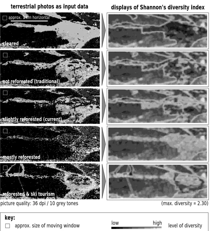
calculation in which Shannon’s diversity index acted as an independent predictor variable for scenic beauty. For example, Figure 6 shows the scenic beauty as-sessments of a terrestrial overview image depicting different reforestation scenarios. It is evident from the images that the scenario 3, labelled ‘mostly reforested’ is most favourable since it has the highest amount of diverse – and therefore beautiful – areas (light pixels). The displayed assessments were then graphically compared with assessments where contagion, domi-nance and total edge acted as predictor variables in alternative monofactorial models. A strong intercor-relation between the predictor variables caused the graphics to have a high degree of resemblance.

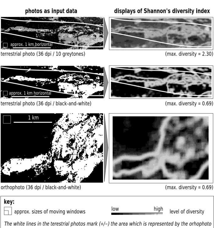
As stated above, such terrestrial overview images are not very useful in landscape planning because im-plementing planning measures requires locating the perimeter on orthogonal maps and plans. For this rea-son, the same ‘moving-window’ procedure was per-formed on an orthophoto. In the orthophoto only two grey tones are indicated, representing either woodland (black) or open land (white). The information was re-duced in this way using computer-aided photo editing. Figure 7 shows the results of calculating Shannon’s diversity index for an orthophoto. The orthogonal quality of the image allows us to call this document a diversity map of the test-region investigated. Also, because there was a close relationship between this index and landscape preferences, the map can also be interpreted to be a prototypical preference map of this region.

Discussion and conclusions

In this paper we have attempted to (a) relate the vi-sual assessment of different stages of a landscape with objectively measured values of the landscape pattern and (b) develop a prototypical technique for rapid au-tomated assessment of landscape changes caused by changing agricultural activities. Before drawing any final conclusions, the advantages and disadvantages of the approach and its limitations should be discussed:

(1) This study is focused solely on the problem of spontaneous reforestation and was carried out using one landscape type. The validity of the presented prototypical instrument is therefore re-stricted to similar cases. By including various differing landscape types and phenomena of land-scape change, however, the instrument’s validity and applicability could be broadened.

(2) The number of landscape elements considered was restricted to trees, shrubs and open land. Thus, we only varied the formal content and did not vary the informal content of the images. It would be challenging, however, to repeat the experiment us-ing different informal content elements, such as houses or roads in rural areas or in expanding urban areas. Furthermore, the influence of the in-formal content on landscape assessments could be investigated if the value of a convenient measure of landscape pattern (formal content) were held con-stant for a landscape and the informal contents of the landscape elements were varied.

(3) The study shows that the scenic beauty assess-ment is not dependent on the selected image-assessing methods, since both the scoring and the pair-comparison method yielded similar results (Schroeder 1984; Stamps 1997; Zube et al. 1974). To carry out the image experiments in a practi-cal manner, the scoring procedure should therefore be preferred to the pair-comparison method, be-cause respondents can assess more images within the same processing time. The scoring procedure does, however, have the statistical disadvantage of relying on the ordinal scale. That problem can be solved using non-parametric procedures or log-linear models.

It is clear from evidence gathered that electron-ically edited photos yield scenic beauty assess-ments that can be safely interpreted as if they had been derived from traditional experiments using real photographs. Furthermore, the results of the image assessments correspond well with those of the exploratory research phase (Hunziker 1995), despite the fact that completely different methods were applied. This indicates the validity of both the qualitative interviews and the image experiments. Also image quality (colour and resolution) seems to have no influence on the assessment of land-scape images, as suggested by other authors (Bishop and Leahy 1989; Daniel and Boster 1976; Jarvis 1990; Nohl 1974; Oh 1994; Stamps 1997). This fact supports the general feasibil-ity of the rapid automated technique using b&w photographs.

(4) The way the pattern indices estimate landscape complexity obviously yields a linear relationship between complexity of the formal content and scenic beauty. This is principally in accordance with the theoretical model of Kaplan et al. (1972, 1989), which also claims a linear relationship

be-reforested & ski tourism

mostly reforested

not reforested (traditional)

cleared

slightly reforested (current)

approx. size of moving window

low

high

level of diversity

key:

displays of Shannon's diversity index

terrestrial photos as input data

(max. diversity = 2.30)

picture quality: 36 dpi / 10 grey tones

approx. 1 km horizontal

Figure 6. ‘Moving-window’ calculation of Shannon’s diversity index for terrestrial grey-tone images of the whole region exhibiting various

terrestrial photo (36 dpi / 10 greytones)

(max. diversity = 2.30)

terrestrial photo (36 dpi / black-and-white)

(max. diversity = 0.69)

(max. diversity = 0.69)

orthophoto (36 dpi / black-and-white)

displays of Shannon's diversity index

approx. sizes of moving windows

low

high

level of diversity

key:

photos as input data

1 km

approx. 1 km horizontal

The white lines in the terestrial photos mark (+/–) the area which is represented by the orhophoto

Figure 7. ‘Moving-window’ calculation of Shannon’s diversity index for a terrestrial grey-tone image and a black-and-white image of the whole

region as well as a black-and-white orthophoto (all representing the scenario ‘slightly reforested’, i.e., the current stage of reforestation). The black-and-white images only distinguish between open land and trees/forest. The diversity map derived from the orthophoto can be interpreted as a preference map due to the significant positive correlation between diversity and preference.

tween landscape preference and complexity. In that respect we confirmed this part of their theory but with the application of a quantitative measure of complexity independent of the respondents. If Kaplan’s approach of estimating complexity by experts’ ratings (Kaplan et al. 1972, 1989) had been applied to our series of images, we believe that the images exhibiting the stages of scenario 4 and scenario 5 would have received overestimated complexity values. This in turn would have lead to a curvilinear relationship (inverted U) between complexity and preference. Further research is re-quired to check whether this assumption can be supported.

(5) Note that the preference maps resulting from the ‘moving-window’ technique are only valid for viewers with average preference profiles. These are indicated by the values shown in Figure 3. Obviously, it might be possible to find individ-uals who would take positions that differ quite significantly from those with average profiles. (6) It is obvious that in a further research step

more explanatory variables should be included in an empirical regression model between prefer-ence values and landscape properties to increase the explained variance of the preference ratings (presently 36%) and to improve the quality of the derived preference map. We did not intend to con-struct such a model for the following reasons: The construction of such a model requires full access to explanatory variables other than pattern indices (e.g., colour ratings, informal contents of the land-scape, etc.). These data, however are not available at the moment.

The inclusion of more than one pattern index for the construction of a multifactorial regression model would probably increase the amount of explained variance but is not justified since the dif-ferent pattern indices are strongly correlated due to formal resemblance of the algorithms.

Considering the limitations described above, we can draw some conclusions. We have concluded that image experiments using computer-edited, simulated images yield the same results as investigations using real scenes and are, thus, valid tools for evaluating the lay assessment of landscape changes in broad surveys. Thanks to the significant relationship between visual preferences of landscapes and indices that measure landscape pattern (formal content) we recommend the developed procedure as a simple tool to predict scenic beauty, on both a meso- and a macro-scale and using

either terrestrial or aerial photographs. However, the prototypical approach presented here needs to be im-proved further if it is to be applied effectively in the practice of landscape planning.

Acknowledgements

We are very grateful to Silvia Dingwall (University of Zürich, CH) for the translation and review as well as to Deborah Barnes (Oak Ridge National Laboratory, USA) for language check and review of the paper, and to the anonymous reviewers as well as to the editor-in-chief, who contributed considerably to the quality of the paper. We also wish to express our thanks to sev-eral professors and teachers who allowed us to conduct the experiments with their students. Susi Tanner (FSL) helped in digitising the questionnaire data.

References

Anwander, S., Buergi, S., Cavegn, G., Meyer, L., Rieder, P. and Salmini, J. 1990. Direktzahlungen an die Berglandwirtschaft. Verlag der Fachvereine an den schweizerischen Hochschulen und Techniken, Zürich.

Baker, B.D. 1996. Landscape pattern, spatial behavior, and a dynamic state variable model. Ecol Model 89: 147–160. Bishop, I.D. and Hulse, D.W. 1994. Prediction of scenic beauty

using mapped data and geographic information systems. Landsc. Urban Plan 30: 59–70.

Bishop, I.D. and Leahy, P.N.A 1989. Assessing the visual impact of development proposals: the validity of computer simulations. Landsc J 8: 92–100.

Bourassa, S.C. 1991. The Aesthetics of Landscape. Belhaven Press, London and New York.

Brown, T. 1994. Conceptualizing smoothness and density as land-scape elements in visual resource management. Landsc Urban Plan 30: 49–58.

Burel, F. and Baudry, J. 1995. Species biodiversity in changing agri-cultural landscapes: A case study in the Pays d’Auge, France. Agric Ecosyst Environ 55: 193–200.

Dale, V.H., Pearson, S.M., Offerman, H.L. and O’Neill, R.V. 1994. Relating patterns of land-use change to faunal biodiversity in the central Amazon. Conserv Biol 8: 1027–1036.

Daniel, T.C. and Boster, R.S. 1976. Measuring landscape aesthet-ics: the scenic beauty estimation method. US Forest Service Research Papers, RM-167.

Flamm, R.O. and Turner, M.G. 1994. Alternative model formula-tions for a stochastic simulation of landscape Change. Landsc Ecol 9: 37–46.

Friedrichs, J. 1985. Methoden empirischer Sozialforschung. West-deutscher Verlag, Opladen.

Gardner, R.H., Milne, B.T., Turner, M.G. and O’Neill, R. 1987. Neutral models for the analysis of broad-scale landscape pattern. Landsc Ecol 1: 19–28.

Gustafson, E.J. and Parker, G.R. 1992. Relationships between land cover proportion and indices of landscape spatial pattern. Landsc Ecol 7: 101–110.

Hadrian, D.R., Bishop, I.D. and Mitcheltree, R. 1988. Automated mapping of visual impacts in utility corridors. Landsc Urban Plan 16: 261–283.

Haider, W. 1994. The aesthetics of white pine and red pine forests. For Chron 70: 402–410.

Hoisl, R., Nohl, W., Zekorn, S. and Zöllner, G. 1987. Landschaft-sästhetik in der Flurbereinigung – Empirische Grundlagen zum Erlebnis der Agrarlandschaft. Materialien zur Flurbereinigung 11.

Hollenhorst, S.J., Brock, S.M., Freimund, W.A. and Twery, M.J. 1993. Predicting the effects of gypsy moth on near-view aesthetic preferences and recreation appeal. For Sci 39: 28–40.

Hulshoff, R.M. 1995. Landscape indices describing a Dutch land-scape. Landsc Ecol 10: 101–111.

Hunziker, M. 1992. Tourismusbedingte Landschaftsveränderungen im Urteil der Touristen. Geogr Helv 4/1992: 143–149. Hunziker, M. 1995. The spontaneous reafforestation in abandoned

agricultural lands: perception and aesthetical assessment by locals and tourists. Landsc Urban Plan 31: 399–410.

Jarvis, D. 1990. Computers in practice – a five year review. Landsc Design, November 1990: 35–37.

Kangas, J., Laasonen, L. and Pukkala, T. 1993. A method for es-timating forest landowner’s landscape preferences. Scand J For Res 8: 408–417.

Kaplan, R., Kaplan, S. and Brown, T. 1989. Environmental prefer-ence – A comparison of four domains of predictors. Env Behav 21: 509–530.

Kaplan, S. 1979. Perception and landscape: conceptions and mis-conceptions. In Proceedings of Our National Landscapes: A Conference on Applied Techniques for Analysis and Manage-ment of the Visual Resource, USDA Forest Service General Technical Report PSW-35, Pacific Southwest Forest and Range Experiment Station, Berkeley, CA.

Kaplan, S., Kaplan, R. and Wendt, J.S. 1972. Rated preference and complexity for natural and urban visual material. Percept Psychophys 12: 354–365.

Lamb, R.J. and Purcell, A.T. 1990. Perception of naturalness in landscape and its relationship to vegetation structure. Landsc Urban Plan 19: 333–352.

Li, H.B. and Reynolds, J.F. 1993. A new contagion index to quantify spatial patterns of landscapes. Landsc Ecol 8: 155–162. Liu, J.G. 1993. Ecolecon – An ecological economic model for

species conservation in complex forest landscapes. Ecol Model 70: 63–87.

McGarigal, K. and Marks, B.J. 1994. FRAGSTATS – Spatial pattern analysis program for quantifying landscape structure. Oregon State University. (ftp://ftp.fsl.orst.edu/pub/fragstats.2.0/) Naiman, R.J., Decamps, H. and Pollock, M. 1993. The role of

ripar-ian corridors in maintaining regional biodiversity. Ecol Appl 3: 209–212.

Nassauer J.I. 1992. The appearance of ecological systems as a matter of policy. Landsc Ecol 6: 239–250.

Nassauer, J.I. 1989. Agricultural policy and aesthetic objectives. J Soil Water Conserv 44: 384–387.

Nohl, W. 1974. Eindrucksqualitäten in realen und simulierten Grü-nanlagen. Landschaft+Stadt 4/1974: 171–187.

Nohl, W. 1982. Über den praktischen Sinn ästhetischer The-orie in der Landschaftsgestaltung - dargestellt am Beispiel der Einbindung baulicher Strukturen in die Landschaft. Landschaft+Stadt 14: 49–55.

Nohl, W. 1988. Naturorientierung als Planungsvariable – Entwick-lung eines Verfahrens zur Erfassung des Naturbewusstseins. Nat Landsch 63: 106–111.

Oh, K. 1994. A perceptual evaluation of computer-based landscape simulations. Landsc Urban Plan 28: 201–216.

O’Neill, R.V., Gardner, R.H. and Turner, M.G. 1992. A hierarchical neutral model for landscape analysis. Landsc Ecol 7: 55–61. Osgood, Ch.E. 1952. The nature and measurement of meaning.

Psychol Bull 49.

Peccol, E., Bird, A.C. and Brewer, T.R. 1996. GIS as a tool for assessing the influence of countryside designations and planning policies on landscape change. J Env Manage 47: 355–367. Pinto-Correia, T., Lourenço, N., Mormont, M. and Sørensen, E.M.

The future of rural marginal areas in Europe: farmer’s attiudes and resulting landscapes (in press).

Plotnick, R.E., Gardner, R.H. and O’Neill, R.V. 1993. Lacunarity indices as measures of landscape texture. Landsc Ecol 8: 201– 211.

Purcell, A.T. 1987. Landscape perception, preference and schema discrepancy. Env Plan B: Plan Des 14: 67–92.

Qi, Y. and Wu, J.G. 1996. Effects of changing spatial resolution on the results of landscape pattern analysis using spatial auto correlation indices. Landsc Ecol 11: 39–49.

Raba, A. 1997: Historische und landschaftsökologische As-pekte einer inneralpinen Terrassenlandschaft am Beispiel von Ramosch. Dissertation, University of Freiburg i.B., Germany. Ribe, R.G. 1994. Scenic beauty perceptions along the ROS. J Env

Manage 42: 199–221.

Ruzicka, M. 1993. Biotopes mapping, base for research of biodiver-sity. Ekologia – Bratislava 12: 325–328.

Schippers, P., Verboom, J., Knaapen, J.P. and Vanapeldoorn, R.C. 1996. Dispersal and habitat connectivity in complex heteroge-neous landscapes: an analysis with a GIS-based random walk model. Ecography 19: 97–106.

Schroeder, H.W. 1984: Environmental perception rating scales: a case for simple methods of analysis. Env Behav 15: 573–598. Schroeder, H.W. 1986. Estimating park tree densities to maximize

landscape esthetics. J Env Manage 23: 325–333.

Schumaker, N.H. 1996. Using landscape indices to predict habitat connectivity. Ecology 77: 1210–1225.

Shafer, E.L., Hamilton, J.F. and Schmidt, E.A. 1969. Natural landscape preferences: a predictive model. J Leisure Res 1: 1–9. Simpson, E.H. 1949. Measurement of diversity. Nature 163: 688. Stamps, A.E. 1997. Meta-analysis in environmental research.

EDRA 28: 114–124.

Steinitz, C. 1990. Toward a sustainable landscape with high visual preference and high ecological integrity: the loop road in Acadia National Park, USA. Landsc Urban Plan 19: 213–250. Turner, M.G. 1990. Landscape changes in nine rural counties in

Georgia. Photog Eng Remote Sensing 56: 379–386.

Turner, M.G., Hargrove, W.W., Gardner, R.H. and Romme, W.H. 1994a. Effects of fire on landscape heterogeneity in Yellowstone National Park, Wyoming. J Veg Sci 5: 731–742.

Turner, M.G., Romme, W.H. and Gardner, R.H. 1994b. Landscape disturbance models and the long-term dynamics of natural areas. Nat Ar J 14: 3–11.

Turner, M.G., Wu, Y.G., Romme, W.H. and Wallace, L.L. 1993. A landscape simulation model of winter foraging by large ungu-lates. Ecol Model 69: 163–184.

Zube, E.H. 1973. Rating the everyday rural landscapes of the north-eastern United States. Landsc Arch July 1973: 370–375. Zube, E.H., Pitt, D.G. and Anderson, T.W. 1974. Perception and

prediction of scenic resource values in the North-East. Amherst, Massachusetts: Institute for man and his environment, University of Massachusetts, publication R-74-1.