HAL Id: hal-03004353
https://hal.archives-ouvertes.fr/hal-03004353
Preprint submitted on 13 Nov 2020
HAL is a multi-disciplinary open access archive for the deposit and dissemination of sci-entific research documents, whether they are pub-lished or not. The documents may come from teaching and research institutions in France or abroad, or from public or private research centers.
L’archive ouverte pluridisciplinaire HAL, est destinée au dépôt et à la diffusion de documents scientifiques de niveau recherche, publiés ou non, émanant des établissements d’enseignement et de recherche français ou étrangers, des laboratoires publics ou privés.
Do PTAs with environmental provisions reduce
emissions? Assessing the effectiveness of climate-related
provisions?
Zakaria Sorgho, Tharakan Joe
To cite this version:
Zakaria Sorgho, Tharakan Joe. Do PTAs with environmental provisions reduce emissions? Assessing the effectiveness of climate-related provisions?. 2020. �hal-03004353�
fondation pour les études et recherches sur le développement international ATION REC ONNUE D ’UTILITÉ PUBLIQUE . T EN ŒUVRE A VEC L ’IDDRI L ’INITIA TIVE POUR LE DÉ VEL OPPEMENT E
T LA GOUVERNANCE MONDIALE (IDGM).
OORDONNE LE LABEX IDGM+ QUI L
’ASSOCIE A U CERDI E T À L ’IDDRI. TTE PUBLIC ATION A BÉNÉFICIÉ D ’UNE AIDE DE L ’É TA T FR ANC AIS GÉRÉE P AR L ’ANR A U TITRE DU PR OGR A MME «INVESTISSEMENT S D ’A VENIR»
TANT LA RÉFÉRENCE «ANR-10-LABX
-14-01».
Abstract
The aim of this paper is to assess the effectiveness on climate change mitigation of the climate-related commitments contained in PTAs. Because of a lack of availability of detailed data on PTAs, the academic literature on the role of PTAs with environmental provisions (PTAwEP) in global climate governance remains limited. A novel and detailed database identifying nearly 300 different types of environmental provisions from more than 680 PTAs since 1947 allows us to establish per country and per year the number of PTAs by distinguishing PTAs with climate-related provisions (PTAwCP) and PTAs with provisions related to other environmental issues. Using panel data covering 165 countries over the period 1995 to 2012, controlling for endogeneity issues, our main result shows that PTAwCP statistically reduce the level of CO2, CH4 and N2O. This suggests that governments seem to comply with the climate-related commitments they made in the PTAs, what potentially helps tackling global warming. Moreover, findings show that to be effective in terms of mitigating climate change, a PTAwEP should contain climate-related commitments.
Keywords: Preferential trade agreements, Climate-related provisions, Environmental policy, Greenhouse gases, Global warming, Climate change. JEL: F13, F18, Q51, Q54.
Do PTAs with environmental
provisions reduce emissions?
Assessing the effectiveness of
climate-related provisions?
Zakaria Sorgho
│Joe Tharakan
Zakaria Sorgho, Laval University and FERDI. Email : zakaria.sorgho@ecn.ulaval.ca Joe Tharakan, HEC-Liège and CORE. Email : j.tharakan@uliege.be
De
velop
ment P
oli
cie
s
Wo
rking
274
Paper
October“Sur quoi la fondera-t-il l’économie du monde qu’il veut
gouverner? Sera-ce sur le caprice de chaque particulier? Quelle
confusion! Sera-ce sur la justice? Il l’ignore.”
1. Introduction
The world trade system has seen an increase in the number of preferential trade agreements (PTAs) since the end of the Uruguay Round in the mid-1990s. While there were 124 before 1995, the number of PTAs has increased rapidly reaching a total number of notifications of 646 at the end of 2016 (Sorgho, 2018). The most common PTAs are concluded in order to reduce (or eliminate) tariffs, quotas and other trade restrictions on items traded between the members. Recent PTAs, in addition to the wide-ranging economic and commercial rules, incorporate a full-length chapter entirely devoted to environmental protection, with precise and enforceable obligations on various environmental issues (Morin et al. 2017).
Many PTAs include obligations not to lower environmental standards, the right to regulate for the benefit of the environment, addressing climate change issues, and the commitment to implement multilateral environmental agreements (MEAs). Nonetheless, the effectiveness of these PTAs to mitigate climate change remains a subject of controversial debate. Some environmentalists are concerned that PTAs will weaken national environmental standards. They see environmental provisions (EPs) as mere “fig leafs” that are included in modern PTAs in order to make them less controversial in the eyes of the public and legislators (Berger et al., 2017). For other critics, PTAwEP represent an instrument of “green protectionism” to keep cheaper products from developing countries out of the market. For others, the inclusion of EPs offers a potential for environmental protection, making these agreements more compatible with environment and climate policies (Berger et al., 2017). For example, PTAwEP can play a role in articulating new environmental norms (Morin et al., 2017) and diffusing environmental policies across borders (Jinnah and Lindsay, 2016). PTAwEP also can help to address trade-related aspects of climate change mitigation, such as the export of low-emission technologies,
border-tax adjustments on polluting production processes, fossil fuel subsidies, and trade in carbon credits (Morin and Jinnah, 2018). Through EPs, PTAs can help to spread cleaner techniques to improve production standards and reduce GHG emissions. Thus, certain authors support the idea that PTAwEP can potentially contribute to climate governance (e.g., OECD, 2007; Whalley, 2011; Leal-Arcas, 2013; Gehring et al., 2013; van Asselt, 2017). This idea is based on the fact that when a given country is linked to an increasing number of countries through PTAwEP, this country could face greater pressure coming from other parties of the PTAwEP to comply with environmental regulations (Martinez-Zarzoso, 2018). However, the effectiveness of a PTA on climate governance depends on whether provisions contained in the agreement address the problem of climate change.
The research on the contribution of PTAs to global climate governance remains yet underexplored (Morin and Jinnah, 2018). Indeed, to the best of our knowledge, few empirical studies have investigated the environmental effects of trade policy using PTAs instead of trade openness.1 While numerous other papers have studied environmental effects of trade policy in
1 Using the trade openness as a proxy for trade liberalization, papers have studied the environmental effects of trade policy (e.g., Antweiller et al., 2001; Cole and Elliot, 2003; Frankel and Rose, 2005; Managi et al., 2009).
the literature,2 because of the problem of lack of detailed data on PTAs, only four papers3 (Ghosh and Yamarik, 2006; Baghdadi et al., 2013; Zhou et al., 2017; and Martinez-Zarzoso and Oueslaty, 2018) have investigated the effects of PTAwEP on pollution levels or environmental outcomes.
Ghosh and Yamarik (2006) proposed an empirical model linking trade, growth and PTAs, and estimated that PTAs can have a direct and an indirect effect (through increasing trade and growth) on the environment. The main limitations of Ghosh and Yamarik (2006) are that they use of single-year data (that does not allow to include the dynamics or to control for unobserved factors that are country-specific and time-invariant) and the fact that they do not deal with how PTAs take into account environmental issues. They do not make the distinction between different types of PTAs, those PTAs with EPs and those without EPs.4 Having omitted this
2 Since Grossman and Krueger (1991), the first paper decomposing the total impact of trade on the environment, several studies (e.g., Brunel and Levinson, 2016; Grether et al., 2009; Levinson, 2009; Managi et al., 2009; Frankel and Rose, 2005; Copeland and Taylor, 2005; Cole and Elliot, 2003; Antweiler et al., 2001) have investigated the impact of trade on environmental quality. The linkages between trade and environment are multiple and complex. The academic literature identifies three channels of transmission of the effects through which trade-led PTAs (liberalizing trade) may affect the environmental quality. As summarized by Sorgho et al. (2018), “the trade impacts on environment through (1) a scale effect: increased economic activity from trade liberalization leads ceteris paribus to increased emissions; (2) a composition effect: trade liberalization may lead to changed specialization patterns across countries and sectors with different emission intensities, which can trigger changes in emissions; (3) a technique effect: through increased income and technology transfer, trade can lead to cleaner production technologies”. For the recent discussion and a literature review on the subject, see Cherniwchan et al. (2017).
3 Other papers (e.g., Yu et al., 2011; Stern, 2007; Logsdon and Husted, 2000; Grossman and Krueger, 1991) have investigated the environmental effects (e.g., energy consumption) of a specific trade agreement (e.g., the North American Free Trade Agreement - NAFTA) at country level (e.g., United states or Mexico).
4 Apart from Carrapatoso (2008), Ferrara et al. (2009), Cai et al. (2013), Baghdadi et al. (2013) and Zhou et al. (2017), most studies on the environment-impact of PTAs do not distinguish PTAs with EPs from PTAs without EPs. Although Carrapatoso (2008), Ferrara et al. (2009), and Cai et al. (2013) do not investigate whether PTAwEP facilitate improvements to the environment, but rather view the trade-related patterns of PTAwEP. Thus, these
distinction could explain the mitigated results Ghosh and Yamarik found regarding the effect of PTAs on the environment.
Later papers refined and extended the modelling strategy established in Ghosh and Yamarik (2006) by considering not only trade and GDP growth as endogenous variables, but also membership in PTAs (e.g. Martinez-Zarzoso and Oueslaty, 2018). Distinguishing PTAs with environmental provisions (PTAwEP) from PTAs without, these papers found that there exists a direct positive effect of PTAwEP on the environment. Focusing on CO2 emissions, Baghdadi et al. (2013) find that PTAwEP not only reduce domestically CO2 emissions, but also lead to a convergence of CO2 emissions across pairs of countries. Conversely, they found that PTAs without EPs do not affect emissions.5 Zhou et al. (2017) examine the effect of PTAs with and without EPs on the concentration of PM2.5, arguing that this is a better indicator of pollution than gross CO2 emissions. They find that PTAs without environmental provisions are associated with worse air quality in terms of PM2.5 concentrations, while PTAs with environmental provisions are likely to lead to lower levels of PM2.5 concentrations. Controlling for national environmental regulations6 – which was not done in Baghdadi et al. (2013) and Zhou et al. (2017) – as well as controlling for scale, composition and technique effects, Martinez-Zarzoso and Oueslaty (2018) found that countries that have ratified RTAs with EPs show lower levels of PM2.5 concentrations. Also, the PM2.5 concentrations in the pairs of countries that belong
papers find that larger countries tend to form environmentally friendly trade agreements in order to collaborate on trade-related environmental issues and minimize their impact on trade.
5 Also, Martinez-Zarzoso and Oueslaty (2016) found that membership in PTAs with EPs is in general associated with higher environmental quality in absolute terms, whereas no significant results are found for PTAs without EPs.
6 The indicator is a composite country specific measure of environmental policy stringency (ESPI) calculated by OECD, covering only 24 OECD countries plus the 6 BRIICS for the period 1990–2012. Also, since ESPI indicator is only available for the small sample of countries, it is almost unchanged over time. Thus, it’s not added in our analysis.
to an RTA with EPs tend to converge for the country sample. In addition to PM2.5, Martínez-Zarzoso (2018) also found similar results for other pollutants such as SO2, NOx and CO2.
Thus, the direct effect of PTAs is explained by the fact that EPs in trade agreements will encourage members to apply and enforce more stringent environmental regulations and these should in turn enhance environmental quality (Martinez-Zarzoso, 2018). But, this direct effect is an average effect for all PTAwEP while EPs included in PTAs are very heterogeneous: some PTAs include EPs that are relative to various areas of environment (such as biodiversity, desertification, hazardous waste, forestry, GHG emissions, or ozone depletion) and others only mention the environment in the investment chapters (see OECD, 2007). Some PTAs include climate-related provisions clearly dedicated to address climate change and in, particular, the mitigation of GHG emissions. This raises the question of whether all PTAwEP have an impact on GHG emissions reduction or whether the effect of PTAwEP on GHG emissions is due to climate-related provisions (CP). Because of a lack of detailed data on PTAs, this question has not yet been studied in previous papers on the role of PTAs with environmental provisions in global climate governance.
A novel and detailed database (“TRade and ENvironment Database” – TREND) identifying
nearly 300 different types of environmental provisions from more than 680 PTAs since 1947 allows us to establish per country and per year the number of PTAwEP containing (or not) climate-related provisions that have been signed. Thus, we distinguish two types of PTAwEP: (i) trade agreements with climate-related provisions (PTAwCP) and (ii) trade agreements with
provisions related to other environmental issues. That allow us to assess whether there is a
causal relation between countries’ climate-related commitments through PTAs they sign and their GHG emissions. Due to the nature of data, we cannot assess the impact of the different-types of environmental provisions (into PTAs) in addressing climate change. Also, our paper
does not assess the impact of trade-led PTAs on environmental quality (e.g., Nemati et al., 2016; and Lovely and Popp, 2011).7
Our main result is that PTAwCP statistically reduce the level of per-capita GHG emissions (CO2, CH4 and N2O). Moreover, the results show that it is rather the climate-related provisions (CPs) in PTAwEP that positively affect the environmental quality. Once purged from effect of climate-related provisions, the impact of PTAwEP have an inconclusive effect with regard to the reduction of GHG emissions. This evidence suggests that to be effective in terms of mitigating climate change, PTAwEP should contain climate-related commitments.
The rest of the paper is structured as follows. The section 2 discuses the heterogeneous nature of environmental provisions contained in PTA. The section 3 presents our empirical framework while section 4 describes and analyses the data used for study. The results and robustness check are presented in section 5. The last part of the paper (section 6) provides a conclusion of the study.
2. Heterogeneity of PTAwEP
A detailed analysis of the database TREND reveals nearly 300 different types of environmental provisions contained PTAs. From the more than 688 PTAs listed between 1947 and 2016, we
7 The academic literature suggests that free-trade deals have an impact on the emission of pollutants. For example, an economic integration can increase the access to environmentally friendly technologies, and lead to earlier adoption of these technologies. Firms are more likely to increase their pollution abatement efforts because of the reduced prices resulting from an import tariff cut induced by trade liberalization (Nemati et al., 2016). However, the environmental effect of a free trade agreement depends on the agreement type. Assessing their impact on world GHG emissions, Lovely and Popp (2011) find that PTAs among only developed or only developing countries can be beneficial for the environment quality while this is not the case when PTAs cover both developing and developed countries.
identify 222 agreements that include at least one provision relating to the environment (so-called PTAwEP). However, environmental provisions (EPs) included in PTAs are very heterogeneous: some PTAs include EPs that are very detailed while others only include general objectives. As in Morin and Jinnah (2018), we can group EPs into eight categories referring to a specific environmental issue: biodiversity8, water, waste, fisheries, forest, dessert, ozone, and climate change. Among these 222 PTAwEP, only 98 agreements (14% of PTAwEP) contain provisions addressing the question of climate change. However, the rate of PTAs with climate-related provisions (PTAwCP) has remarkably increased since 2010, even if it still remains small compared to the number of PTAwEP.
As Figure 1 shows since 1970, the share of PTAs negotiated on a bilateral and regional basis that have comprehensive environmental-related components has increased. In 1970, more than 50 per cent of all PTAs already contained environmental provisions (EPs). In 2012, the number of PTAs with EPs (PTAwEP) represented more than 85 per cent of all PTAs. Some PTAs include climate-related provisions to address climate change. The inclusion of provisions in PTAs addressing specifically climate issues was quite limited until 1990.9 Before this date, the number of PTAs with climate-related provisions (PTAwCP) was about 18 per cent of total of PTAs. Since 1990, the number of PTAwCP has increased rapidly. It represents now about 55 per cent of total of PTAs.
8Biodiversity provisions include provisions related to endangered species, invasive species, migratory species,
protected areas, genetic resources, biosafety and genetically modified organisms (Morin and Jinnah, 2018).
9 Maybe a coincidence, 1990 is the date of the first report of the IPCC (Intergovernmental Panel on Climate
Change) – an international scientific body set up in 1985 – that points out that human activities emit pollutants that significantly increase the concentration in the atmosphere of greenhouse gases (carbon dioxide, methane, chlorofluorocarbons, nitrous oxide) and enhance the natural greenhouse effect.
Given this evolution, the main interest of our paper is to take into account the heterogeneity of PTAwEP. Unlike previous papers, our paper assesses the impact of climate-related provisions (included in PTAs) on climate change mitigation through the reduction of GHG emissions including CO2, CH4 and N2O, responsible for global warming which is a major element of climate change.10 In doing so, we investigates whether the effect of PTAwEP on GHG emissions (found in previous studies) is due to the specific commitments of countries on climate change. Thus, our study distinguishes PTAs with climate change provisions (PTAwCP) from other PTAwEP.
Figure 1. Overview of Preferential trade agreements (PTAs)
Source: Authors, created with data from “TRade and ENvironment Database” – TREND. Note: PTAwEP means PTAs with environmental provisions; PTAwCP means PTAs with climate-related provisions.
10 As Sorgho et al. (2018), we do not include in the study Fluorinated gases (F-gases) as Chlorofluorocarbons (CFC), Sulfurhexafluoride (SF6), Hydrofluorocarbons (HFC) and Perfluorocarbons (PFC). These environment-harmful substances (F-gases) are almost totally prohibited since the entry in force of Montreal Protocol in 1989.
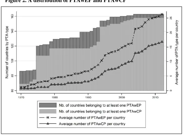
Figure 2 shows the evolution of the interest of countries in environmental issues. It shows an increasing number of countries belonging to agreements that include at least one climate change provision. This shows that many countries become aware of the climate issue. While until 1995 this was less than 5 PTAwCP, since 2008, on average, a country belongs at least to 15 PTAwCP.
Figure 2. A distribution of PTAwEP and PTAwCP
Source: Authors, created with data from “TRade and ENvironment Database” – TREND.
Considering the various environmental areas addressed by PTAs through EPs, PTAwCP are more specific and efficient to address the problem of climate change. These climate commitments included in PTAs are those that affect environmental quality once they have been implemented into national legislation. Governments have incentives (or will be constrained) to comply with commitments made in PTAwCP to which they are a Party. There is evidence of a positive and significant direct link between a country signing PTAs with many comprehensive EPs and a country introducing more environmental legislation domestically (see Brandi et al.,
2019; George and Yamaguchi, 2018).11 In our data, several PTAwCP address explicitly the climate change issues with clauses even more specific and restrictive than those found in MEAs. For example, more than 50 PTAwCP include innovative climate provisions more specific and enforceable than the Kyoto Protocol and the Paris Agreement. This suggests a potential causal relationship between signing PTAwCP and GHG emissions: these gases would be reduced because countries implement international commitments on environmental issues into domestic legislation.
3. Modelling Framework
3.1. Empirical Model
The objective of this paper is to determine whether PTA-commitments on climate change issues have had an impact on the environmental quality through a reduction of emissions of the main greenhouse gases (GHG): emissions of CO2, CH4, and N2O. We adopt an environmental quality model. As well-discussed in the empirical literature on “trade policy and environment”, we control for scale, technique and composition effects in order to assess the effect of PTAwCP on emissions of GHG. Our model includes the usual determinants of emissions such as population density, per capita GDP and trade openness (e.g., Martinez-Zarzoso and Oueslaty, 2018; Zhou et al., 2017; Cherniwcha et al., 2017; Baghdadi et al., 2013; Managi et al., 2009; Frankel and Rose, 2005; Copeland and Taylor, 2005). It is a dynamic panel data model incorporating the
11 In particular, George and Yamaguchi (2018) find that the United States and the European Union have made significant steps towards setting what may be regarded as a benchmark for monitoring and reporting on the implementation of environmental provisions in PTAs.
temporal dependency of the dependent variable on the past (noted by g1 it
Em ). Our model includes climate-related commitments as follows:
0 1
1
2
3
4 5
log log log
log log g it it it g it pta it it t it Em Popdens Open Em GDPcap Reg FE (1)
where Em denotes the per-capita emissions of each pollutant-type “g” (either CO2, CH4, or itg N2O) from country i at the period t. Our dependent variable is measured in kilograms of emissions “g” per capita. The variable (Openit), which proxies trade openness (i.e., trade intensity), is defined as the sum of trade (exports + imports) over GDP. This variable helps to capture the potential direct effect of trade openness on the environmental quality. Its effect could be positive or negative on environmental quality. The other control variables are
Popdensit
for population density measuring the number of inhabitants per square kilometers(Km2) in country i in year t,
GDPcapit
for GDP per capita at constant US dollars in countryi in year t. The variable
Popdensit
is used as a proxy for the scale effect. We add country fixed effects and time fixed effects (FEt) to capture the linear time-trend effects (temporal events independent of countries). The term
it is the error term consists of an individual country effect i and a random disturbance
it (
it i
it).According to previous studies, the coefficient of g 1 it
Em is intuitively expected to have a positive sign (e.g. Martinez-Zarzoso and Oueslaty, 2018; Managi et al., 2009). The coefficients for “per-capita GDP” and “trade openness”, measuring their impact on CO2 emissions, are also expected to be positive (e.g. Baghdadi et al., 2013). Indeed, the literature intuitively assumes that the more a country is populous, economically rich, and/or commercially open, the more it pollutes
(in absolute term). However, a high concentration (of inhabitants) per km² can lead to some form of economy of scale in terms of pollutant emissions. Accordingly, a country with a high population density can have a low emission per capita.
Through stringent environmental regulations, a country could have lower emissions despite its comparative advantage in capital-intensive goods (i.e., having a high capital-labor ratio). The domestic productive units would be constrained by the strict environmental standards (implemented by country) and adopt new more environment-friendly technologies and practices.
The variable Regitpta represents the environment-related commitments embodied by the PTAwEP (or specifically climate-related commitments into PTAwCP) signed by a country i in year t. By including climate-related provisions in almost all PTAs it signs, a government signals its strong interest for climate change issues. Indeed, there is a positive relationship between international obligations on specific environmental issue areas and domestic environmental legislation in the same issue areas (see Brandi et al., 2019; George and Yamaguchi, 2018). To avoid paying environmental compliance costs (when international commitments on environment/climate will be incorporated into domestic law), companies can anticipate by adopting environment-friendly technologies and practices. Thus, PTAwCP could benefit the environmental quality by lowering pollutants’ emissions (i.e., an indirect negative relationship between PTAwCP and GHG emissions). This negative effect on emissions is captured by the coefficient associated to Regitpta.
Instead of a simple dummy12 indicating a PTAwEP (or PTAwCP), we define our variable of interest (Regitpta) as the number of PTAwEP (or the number of PTAwCP). We consider multi-commitments through different PTAs (involving various partners) as a proxy measuring the willingness of a country to deal with climate change issues. Thus, we introduce the number of PTAwEP (or the number of PTAwCP) into the estimating equation (1) above.13 Taking the number of PTAwCP, rather than a dummy reflecting whether or not a country has a PTAwCP, allows to address the selection bias problem of PTAs. All countries are included in the analysis.
3.2. Pre-treatment for the endogeneity problem
As emphasized by the literature, the variables “GDP” and “trade openness” may be endogenously determined with environmental regulation (e.g., Martinez-Zarzoso and Oueslaty, 2018; Zhou et al., 2017; Baghdadi et al., 2013; Managi et al., 2009; Frankel and Rose, 2005).14 Moreover, certain covariates like trade (trade openness) and production (GDP) may be simultaneously contributing to regulatory stringency (an explanatory variable) and our dependent variable “pollutants’ emissions” (Brunel and Levinson, 2016). Consequently, we first instrument these variables by using a set of instrumental variables. We adopt an income equation (see equation 3) taken from the growth literature to instrument the variable “GDP” for each country (the predicted values of GDP). For the “trade openness”, we run a gravity model
12 Previous studies on the environment-impact of PTAs (e.g. Baghdadi et al., 2013) design the variable of interest as a dummy variable taking a value of 1 if country is involved in a PTA in the considered year, and zero otherwise.
13 Using for our variable of interest a dummy variable (indicating whether country belongs to a PTA) would not be suitable in our case. In general, a PTA dummy depends on pairs of countries, while in this study the data is by country.
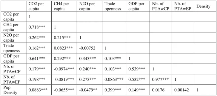
14 The correlation matrix in Table A1 suggests that all explanatory variables in equation (1) are not exogenous; e.g., “per-capita GDP”, and “trade openness” are highly correlated with our interest variable (e.g., Nb. of PTAwCP).
with pair-wise trade. The predicted values of aggregated bilateral trade (all trade) is used to calculate the openness for a given country (see equation 4). This instrumentation approach seeks to deal with both endogeneity and simultaneity problems pointed out above (e.g. Milllinet and Roy, 2016).
We use the predicted values of “income” (GDPit) (i.e., the predicted values of GDP instead of its observed values) and “trade openness” (Openit) (i.e., the predicted values of trade openness instead of its observed values) as instrumented variables in the equation (1).
In the equation (3), inspired from the growth-literature, we run an OLS model to regress an income equation on all trade
Tradeit
, investments
Invit
calculated as the stock of inward foreign direct investments (FDIs), population (Popit)and human capital
Sch approximated it
by the rate of school enrolment. With an error term (
it), the income equation is:
0 1
2
3
4
log GDPit log Tradeit log Invit log Popit log Schit FEtit
(3)
The variable Trade represents the yearly sum of exports plus imports for a country i at time t, it
as follows: it ijt ijt
j j
Trade
Export
Imports (where ijtj Exports
and ijt j Imports
arerespectively the total exports and the total imports, at period t. After the estimation of equation (3), we predict values of GDP for each country at year t (noted GDPit).15
15 As the predicted values of GDP directly obtained from the OLS estimation (3) are in logarithmic form, we transform them by taking their exponential in order to have the predicted values needed.
Following the literature, we adopt a gravity approach to create an instrumental variable for “trade openness” (e.g., Baghdadi et al., 2013; Frankel and Romer, 1999). We implement a PPML16 gravity model that explains bilateral trade between two trading partners by their size (GDP and population) and distances between them (physical distance and dummy variables indicating common borders and linguistic link status).
0 1 2 3
4 5 6 7
log log log
log log ij it jt ijt it jt ij ij t ijt dist GDP GDP T Pop Pop CB CL FE (4)
Here, T denotes the bilateral trade (exports plus imports) of two trading partners i and j at the ijt period t. The productions (GDPitandGDP ) and the populations (jt PopitandPop ) are jt respectively referred to countries i and j; and dist is the physical distance between them. In ij additional, the dummy variables:CB takes the value of 1 if both countries i and j share a ij common border and 0 otherwise; and CL takes the value of 1 if both countries i and j share a ij
common language and 0 otherwise. We also include temporal fixed effects
FEt to control forthe time trend. The term (
ijt) is an error term. After predicting values of bilateral trade T ijtfrom equation (4), we aggregate them to obtain a prediction for total trade (T ) for each country it at year t, as follows:Tit
Tijt (where terms
Tijt is the sum of predicted bilateral trade, at period t). Then, we use the values of T to calculate the “trade openness” (it Openit) for each
16 Silva and Tenreyro (2006) suggest the PPML estimator in order to deal with the presence of heteroscedasticity and take into account the problem of zero (generally) observed in trade data. Moreover, in our case, contrast to the OLS model, the PPML gravity model gives directly the predicted values needed because the dependent variable is in level (not in logarithmic form).
country i at year t by dividing them by the predicted value of GDP, i.e. (GDPit) from equation (3).
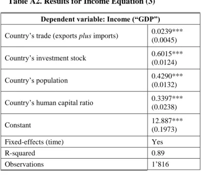
The results from equations (3) and (4) are reported in Appendix A. As reported in Tables A2 and A3 for equations (3) and (4) respectively, all estimated coefficients are statistically significant with the expected sign (with respect to the existing literature).
4. Data description
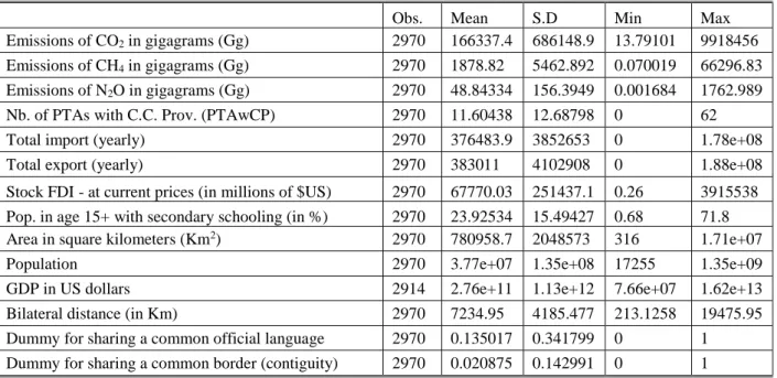
For this study, we construct a dataset from various sources. Table 1 shows the summary statistics for the covariates used. Our dataset covers the period 1995–2012 for 165 countries (for the list of countries, see the Appendix C). Data on trade are from the UN COMTRADE database.17 Data on pollutants’ emissions (CO2, N2O, and CH4) are obtained from the European Commission.18
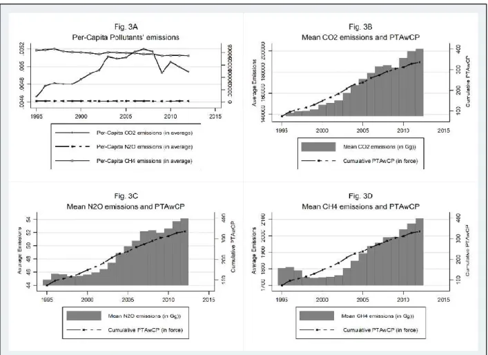
Figure 3 shows that the pollution per capita is more stable for N2O than the per-capita emissions in CO2 and CH4 (see Fig. 3A). However, we can note a decrease of per-capita emissions for CH4 since 1997. The per-capita pollution for CO2 started to decrease from 2008 after a regular increase until 2007. Between 1995 and 2000, the average emission (per country) was relatively stable despite the large number of PTAwCP.
17 World Bank database: http://databank.worldbank.org/data/reports.aspx?source=world-development-indicators [Accessed June 05, 2018].
18 European Commission, Joint Research Centre (EC-JRC)/Netherlands Environmental Assessment Agency (PBL). Emissions Database for Global Atmospheric Research (EDGAR), release EDGAR v4.3.2 (1970 - 2012) of March 2016: http://edgar.jrc.ec.europa.eu [Accessed June 05, 2018].
From 2000, the average emission of pollutants has particularly accelerated; the average emissions of CO2 (see Fig. 3B), and that of N2O (see Fig. 3C) have increased proportionally to the number of PTAwCP, while the evolution of the average emissions of CH4 (see Fig. 3D) is less than proportional to the number of PTAwCP. However, the overview of Figure 3 does not give a conclusive picture of the causal relationship between countries’ GHG emissions and the number of PTAwCP they have signed. Indeed, from these figures, we cannot conclude to any pattern in GHG emissions associated to climate-related commitments into PTAs made by countries.
Figure 3. Evolution of Pollutants’ emissions and PTAwCP
Source: Authors, created using data from “TRade and ENvironment Database” – TREND, and Emissions Database for Global Atmospheric Research (EDGAR).
Table 1. Descriptive statistics
Obs. Mean S.D Min Max
Emissions of CO2 in gigagrams (Gg) 2970 166337.4 686148.9 13.79101 9918456 Emissions of CH4 in gigagrams (Gg) 2970 1878.82 5462.892 0.070019 66296.83 Emissions of N2O in gigagrams (Gg) 2970 48.84334 156.3949 0.001684 1762.989 Nb. of PTAs with C.C. Prov. (PTAwCP) 2970 11.60438 12.68798 0 62
Total import (yearly) 2970 376483.9 3852653 0 1.78e+08
Total export (yearly) 2970 383011 4102908 0 1.88e+08
Stock FDI - at current prices (in millions of $US) 2970 67770.03 251437.1 0.26 3915538 Pop. in age 15+ with secondary schooling (in %) 2970 23.92534 15.49427 0.68 71.8 Area in square kilometers (Km2) 2970 780958.7 2048573 316 1.71e+07
Population 2970 3.77e+07 1.35e+08 17255 1.35e+09
GDP in US dollars 2914 2.76e+11 1.13e+12 7.66e+07 1.62e+13
Bilateral distance (in Km) 2970 7234.95 4185.477 213.1258 19475.95
Dummy for sharing a common official language 2970 0.135017 0.341799 0 1 Dummy for sharing a common border (contiguity) 2970 0.020875 0.142991 0 1
Source: Data are from Emissions Database for Global Atmospheric Research (EDGAR), UNCTAD’s database, World Development Indicators (World Bank), TRade and ENvironment Database (TREND), Centre d’Études Prospectives et d’Informations Internationales (CEPII).
The data on gross national product (GDP), land area, population, school enrollment19 comes from World Development Indicators.20 Data on foreign direct investments (FDIs) are from the UNCTAD’s database.21 The other gravity data, such as bilateral distance, common language and contiguity dummies come from the Centre d’Études Prospectives et d’Informations Internationales (CEPII). Data on trade agreements with climate-related provisions (PTAwCP) come from the TRade and ENvironment Database (TREND). This PTA-database encodes information on the environmental provisions (including the climate-related provisions) contained in 688 PTAs signed between 1947 and 2016. Our definition of PTAwCP follows the
19 This educational attainment data is computed following Barro R. and Lee J.-W. (2013). These authors compute an average index of education ranging from 0 to 1, where 1 represents 16 education-years.
20 All values are in 2005 constant US Dollar.
21 See UNCTAD Stat: http://unctadstat.unctad.org/wds/ReportFolders/reportFolders.aspx?sCS_ChosenLang=fr [Accessed June 05, 2018].
study of Morin and Jinnah (2018) which manually code the climate-related provisions contained in PTAs from TREND. For a list of these climate-related provisions in PTAs, see Appendix B.
5. Estimation strategy and results
As defined in the equation (1), the implementation of our environmental model requires the “dynamic” panel data techniques rather than the “static” panel data methods (e.g., GLS estimation, OLS estimation, and fixed-effects estimation). Even if the static panel data models are robust under heteroskedastic disturbances (Davidson and MacKinnon, 2004), none of them has acceptable properties when a dynamic structure is introduced in the model as in our case.22
Because of the potential issue of endogeneity and reverse causality23 of the PTA variable, it is difficult to isolate the environmental effects of PTAwCP. As in Martinez-Zarzoso and Oueslaty (2018), in order to address the issue of endogeneity and reverse causality of the PTA variable, we estimate by the dynamic Generalized Method of Moments (GMM) for panel data (Arellano and Bond 1991; Blundell and Bond 1998).24 As a robustness check, we estimate a panel data model – as suggested by Baier and Bergstrand (2007) – to control for the endogeneity of the
22Including a lagged dependent variable as a regressor in the equation (1) violates strict exogeneity, because of its
correlation with the idiosyncratic error. Thus, as the strict exogeneity assumption is violated, commonly use of “static” panel data estimators are inconsistent; these estimators require strict exogeneity. Moreover, the
instrumental variables (IV) estimation proposed by Anderson and Hsiao (1982) as a solution (when the strict exogeneity assumption is violated) has been found asymptotically inefficient by Arellano and Bond (1991) who propose a more efficient estimation procedure (using moment conditions in which lags of the dependent variable and first differences of the exogenous variables are instruments for the first-differenced equation).
23 In other words, if we know that the accumulation of PTAwEP may lead to better environmental quality, a country that seeks to improve environmental quality may also be keen to enter into negotiations of PTAwEP.
24The difference GMM estimator uses moment conditions from the estimated first differences of the error term.
While the system GMM estimator utilizes an additional set of level moment conditions as well as the difference moment conditions to estimate dynamic panel data. In our case, the system GMM estimator is not necessary.
PTA variable in the environmental-impact model (equation 1), while using the instrumental method will enable us to address the endogeneity of the income and trade variables (see section 2).
When using panel data, the unobserved country-specific component is eliminated by taking the first differences of the left- and right-hand-side variables and the endogeneity issue is solved by using the lagged values of the levels of the endogenous variables as instruments (Martinez-Zarzoso, 2018). Thus, the estimating equation (1) is transformed as follows:
0 1 1 2 3
4 5
log log log
log log g it it it g it pta it t it it Em Popdens Open Em GDPcap Reg FE (5)
where defines the first difference of the corresponding variable. Open indicates the predicted it value of variable of “trade openness”. GDPcap is predicted value of per-capita GDP. The it other variables in the equation have already been described above for equation (1).
There are two situations where the difference GMM model does not provide good estimators: when model errors are heteroskedastic (see Windmeijer, 2005) and when using time invariant regressors (see Blundell and Bond, 1998).25 Both problems do not matter in our case. Moreover, once difference GMM results are obtained, the validity of the model must be checked: test for serial correlation in the first-differenced residuals and test for the validity of the overidentifying restrictions. In our case, the explanatory variables such as “per-capita GDP” and “trade
25 When model errors are heteroskedastic, Windmeijer (2005) proposes to correct it by implementing the two-step GMM estimator (using thus a first-step estimation to obtain the covariance matrix of estimation error). In the case of time-invariant regressors in the model, the econometric literature proposes to use the system GMM estimator rather than the difference GMM estimator (see Arellano and Bover, 1995; Blundell and Bond, 1998).
openness” that are potentially endogenous have first been instrumented before estimating equation (5).
The validity of specific instruments can be tested in the GMM framework by using the Hansen test of over-identifying restrictions.26 In our analysis, we consider as endogenous variables the lagged dependent variable and the variables related to a PTA with EPs/CPs and the instruments used are the second lagged values of the levels of the respective variables and density of country. The GMM results from equation (5) are reported in Table (2) and FGLS results from equation (1) are shown in Table (3) as robustness test. Results are reported for the following three specifications:
- Specification (1): investigating the environmental-effects of PTAwEP; - Specification (2): investigating the environmental-effects of PTAwCP;
- Specification (3): investigating both effects of PTAwEP (without CP) and PTAwCP.
Specification (1) replicates results from previous studies, while specifications (2) and (3) are our main contribution to literature. The two last specifications seek to show that PTAwEP are heterogeneous with regard to their impact on climate change issues: certain PTAwEP contain general environmental provisions while others are more specific with provisions addressing the problem of climate change. To do that, we split PTAwEP in PTAwEP containing climate-related provisions (noted PTAwCP) and PTAwEP without CP (noted PTAw/oCP). We then isolate the impact of PTAwCP on GHG emissions (specification 2) and test its sensitivity by conjointly running PTAwCP and PTAw/oCP (specification 3) in the same equation.
26 Hansen test: under the null hypothesis (H0), the instruments used to address the endogeneity of some regressors are valid instruments. When the associated probability value is lower than 0.05, the null hypothesis (H0) is rejected.
Before discussing the results regarding our variable of interest (climate-related provisions), we check the validity of GMM estimations. As reported in Tables 2, results on AR-tests (i.e., the non-significance on the hypothesis of no second-order autocorrelation) show that there is no serial correlation in the error term and our GMM estimations are valid. Thus, residuals are uncorrelated with instruments taking the number of PTAwCP as the measure of climate-related commitments in PTAs. Moreover, the results on Hansen test are all insignificant; the null hypothesis (H0) can not be rejected. Thus, the instruments used to address the endogeneity of PTA variable are valid. Overall, these results confirm that the use a dynamic model for our study is justified.
With respect to the control variables, the lagged emissions terms for all specifications are statistically significant with a positive sign and their values are less than one. As concluded by Managi et al. (2009), these results imply that changes in explanatory variables, such as “trade openness” or “per-capita GDP”, at a specific point in time would also influence emissions after the current period. The estimated coefficients on “trade openness” and “per-capita GDP” have the expected sign, even if some of them are non-significant.
Thus, a higher per-capita income (higher GDP per capita) is estimated as having a positive impact on the GHG emissions. The estimated coefficient on the “population density” is significant for all specifications suggesting that a country with a higher concentration of inhabitants per square kilometer (Km²) has lower GHG emissions. The positive estimated coefficient on “trade openness” indicates that a large openness for country tends to increase its GHG emissions. The results confirm that the economically richer the country, the more it tends to pollute. However, the non-significance effect on “trade openness” can be linked to the fact that a participation to PTAwEP or PTAwCP is potentially harmful for free trade.
As concluded by previous studies (e.g. Martinez-Zarzoso and Oueslaty, 2018; Zhou et al., 2017; Baghdadi et al., 2013), our results indicate that pollutants emissions (N2O, CO2 and CH4) are reduced for countries that belong to PTAs with EPs (specification 1 in Table 2).27 We find that each additional PTA with EPs decreases the mean of per-capita emissions by around 1.3% (for CO2), by around 0.7% (for CH4), and by around 1.6% (for N2O), whereas PTA without EP show positive and significant coefficients (except for CH4).28 However, these effects of PTAwEP seem to hide the direct effects of specific PTAs such as PTAwCP as shown in the following analysis.
All the estimated coefficients for the variable “environmental commitments” related to climate change have a negative sign and are highly significant for specifications (2) and (3). Accordingly, we can conclude that multi-commitments on climate change through the signing of several PTAwCP helps the mitigation of emissions responsible for greenhouse gases (GHG). The estimated coefficients on PTA without EP remain similar to those obtained in specification (1), except for CH4 (in specification 3) where the coefficient is negative and not significant.29
In specification (2) in Table 2, the estimated coefficient on PTAwCP displays -0.0181 (for CO2 emissions), -0.0108 (for CH4 emissions), and -0.0211 (for N2O emissions). Thus, these results indicate that signing an additional PTAwCP by a country reduces, on average, its per-capita
27 Baghdadi et al. (2013) found that CO
2 emissions are around 0.3% lower for countries that have RTAs with EPs, whereas the effect is not statistically significant for countries with RTAs without EPs. Martinez-Zarzoso, (2018) found that an additional PTA with EPs can decrease CO2 emissions by 0.4% for countries that have RTAs with EPs.
28 Since our variable of interest is a count variable, the interpretation is slightly different from that of an elasticity. An increase of one unit of this variable increases (decreases in case of a negative coefficient) the dependent variable by beta*100.
29 Recall that our study data cover the period from 1995 to 2012, and more than 80% of all PTAs contain environmental provisions (PTAwEP).
emissions by around 1.8% (about 36.9 metric tons), 1.1% (about 24.2 metric tons), and 2.1% (about 21.1 metric tons) respectively for CO2, CH4 and N2O.30 Comparatively, it is not surprising that the magnitude of the effect of PTAwCP (containing more specific provisions) are higher than that of PTAwEP (that can include simple declarations of good intentions).
In specification (3), we include both PTAwEP and PTAwCP in same equation. The associated coefficient on PTAwCP remains negative and significant, and its amplitude is similar to that obtained in specification (2). However, the effect of PTAwEP without CP (noted PTAw/oCP) is inconclusive. The estimated coefficient on PTAw/oCP is positive and not significant for CO2 emissions, but significant for CH4 emissions, while it is negative but not significant for N2O emissions. The mixed effect of PTAw/oCP on GHG emissions could be due to the heterogeneity of environmental provisions (EPs) that range from declarations of good intentions on environment to environmental provisions that are not necessarily relevant for GHG mitigation.
Table 2. Results of GMM estimates - Causal effect of PTAwCP on Pollutants’ emissions
Specification (1) Specification (2) Specification (3)
CO2 em. CH4 em. N2O em. CO2 em. CH4 em. N2O em. CO2 em. CH4 em. N2O em.
Lag of per-capita emissions 0.3464*** (0.0657) 0.5465*** (0.0572) 0.1693*** (0.0486) 0.3367*** (0.0677) 0.5305*** (0.0596) 0.1496*** (0.0571) 0.3347*** (0.0693) 0.5048*** (0.0593) 0.1516** (0.0617) Trade openness (instrumented) 0.0113 (0.0108) 0.0121 (0.0080) 0.0202** (0.0081) 0.0107 (0.0121) 0.0124 (0.0087) 0.0161** (0.0082) 0.0102 (0.0119) 0.0130 (0.0082) 0.0163* (0.0087) Number of PTAw/oEP 0.1278*** (0.0451) 0.0508 (0.0345) 0.1782*** (0.0427) 0.0923** (0.0356) 0.0473 (0.0287) 0.1190*** (0.0348) 0.0767 (0.0522) -0.0137 (0.0372) 0.1351** (0.0592) Number of PTAwEP -0.0129*** (0.0031) -0.0066*** (0.0021) -0.0162*** (0.0036) – – – – – – Number of PTAw/oCP – – – – – – 0.0043 (0.0125) 0.0178** (0.0072) -0.0037 (0.0158) Number of PTAwCP – – – -0.0181*** (0.0042) -0.0108*** (0.0028) -0.0211*** (0.0047) -0.0193*** (0.0060) -0.0153*** (0.0035) -0.0203*** (0.0065) Pop. density (inhabitants/km²) -0.2259* (0.1303) -0.2591*** (0.0958) -0.3679*** (0.1106) -0.2788** (0.1272) -0.2971*** (0.1054) -0.4340*** (0.1093) -0.2914** (0.1251) -0.3399*** (0.1132) -0.4229*** (0.1257) Per-capita GDP (instrumented) 0.0070 (0.0141) 0.0098 (0.0111) 0.0451*** (0.0138) 0.0006 (0.0142) 0.0048 (0.0110) 0.0278** (0.0141) 0.0009 (0.0142) 0.0059 (0.0112) 0.0283* (0.0153)
Time fixed-effects Yes Yes Yes Yes Yes Yes Yes Yes Yes
R-Squared 0.653 0.762 0.254 0.608 0.733 0.265 0.599 0.699 0.259
Nb. of observations 2,609 2,609 2,609 2,609 2,609 2,609 2,609 2,609 2,609
Nb. of countries 164 164 164 164 164 164 164 164 164
AR(1) -4.41*** -4.54*** -2.98*** -4.21*** -4.28*** -2.66*** -4.13*** -4.15*** -2.52***
AR(2) -0.54 0.22 -1.33 -0.49 0.22 -1.20 -0.48 0.22 -1.23
Hansen Test (Prob) 1.000 1.000 1.000 1.000 1.000 1.000 1.000 1.000 1.000
Notes: Standard errors, in parentheses, are robust to heteroskedasticity and arbitrary patterns of autocorrelation within individuals. The symbols (***), (**) and (*) to coefficients means that latter are respectively significant at the 1% level, 5% level and 10% level. The variables: “trade openness” and “per-capita GDP” are instrumented for using their “predicted” values. Time fixed-effects are not reported. PTAwEP means trade agreement with environmental provisions. PTAwCP means trade agreement with climate-related provisions. PTAw/oEP means PTA without environmental provisions. PTAw/oCP means PTAwEP without climate-related provisions. Variable of interest: PTAwCP as PTA - PTAw/oEP - PTAw/oCP = PTAwEP - PTAw/oCP (with PTAwEP = PTA - PTAw/oEP).
PTA with climate-related provisions (PTAwCP) target better the reduction of gases responsible to climate change. In our data, more than half of PTAwEP are PTAwCP. Thus, having purged the direct effect of PTAwCP on GHG emissions, the coefficient of PTA without CP (PTAw/oCP) is not significant (except for CH4). The positive and significant coefficient for CH4 would mean that effect of PTAw/oCP could be harmful on environment quality as a PTA without EP. Therefore, their impact on the environment should be modulated through trade or income.
As a robustness check, we run equation (1) using panel data techniques (FGLS) as suggested by Baier and Bergstrand (2007). The FGLS results shown in Table 3 follow the three different specifications described above. Except for the coefficient on PTAw/oEP for CO2 emissions (negative and significant)31, the results in Table 3 are similar to Table 2. FGLS estimates also support the idea that climate-related commitments through PTAwCP led to a reduction of per-capita emissions of GHG. For specification (2) in Table 3, the estimated coefficient on our interest variable (PTAwCP) is 0.0071 (for CO2 emissions), 0.0070 (for CH4 emissions) and -0.0112 (for N2O emissions). For all GHG, it is negative and statistically significant. These results remain significantly stable when we conjointly run PTAwCP and PTAw/oCP in same equation (specification 3). This means that signing an additional PTAwCP significantly decreases (on average) the level of per-capita GHG emissions by about 1.4% for CO2 emissions, 0.7% for CH4 emissions and 1.7% for N2O emissions (specification 3).
31 The negative and statistically significant coefficients of PTAw/oEP could be due to the fact that we are not able to control for domestic environmental regulations (Martínez‑Zarzoso and Oueslati, 2018: 761).
Table 3. Results of FGLS estimates - Causal effect of PTAwCP on Pollutants’ emissions
Specification (1) Specification (2) Specification (3)
CO2 em. CH4 em. N2O em. CO2 em. CH4 em. N2O em. CO2 em. CH4 em. N2O em.
Trade openness (instrumented) 0.0124** (0.0056) 0.0206*** (0.0053) 0.0097*** (0.0034) 0.0123** (0.0052) 0.0205*** (0.0053) 0.0098*** (0.0030) 0.0128*** (0.0047) 0.0208*** (0.0056) 0.0102*** (0.0025) Number of PTAw/oEP 0.0004 (0.0207) -0.0046 (0.0169) 0.0625*** (0.0178) 0.0101 (0.0176) 0.0032 (0.0154) 0.0651*** (0.0153) -0.0334* (0.0192) -0.0241 (0.0154) 0.0277* (0.0154) Number of PTAwEP -0.0027* (0.0016) -0.0008 (0.0014) -0.0055*** (0.0016) – – – – – – Number of PTAw/oCP – – – – – – 0.0156*** (0.0045) 0.0098** (0.0040) 0.0134*** (0.0044) Number of PTAwCP – – – -0.0071*** (0.0027) -0.0030 (0.0024) -0.0112*** (0.0025) -0.0142*** (0.0037) -0.0074** (0.0036) -0.0172*** (0.0036) Pop. density (inhabitants/km²) -0.3258** (0.1366) -0.3795** (0.1614) -0.3353*** (0.0997) -0.3776*** (0.1356) -0.4062** (0.1624) -0.3997*** (0.0956) -0.4424*** (0.1371) -0.4469*** (0.1644) -0.4555*** (0.0971) Per-capita GDP (instrumented) 0.0347* (0.0181) 0.0344* (0.0180) 0.0303** (0.0131) 0.0327* (0.0182) 0.0335* (0.0179) 0.0277** (0.0126) 0.0294 (0.0184) 0.0314* (0.0177) 0.0249** (0.0121) Constant -6.238*** (0.3504) -8.392*** (0.4208) -13.452*** (0.2330) -6.087*** (0.3499) -8.313*** (0.4235) -13.268*** (0.2231) -5.919*** (0.3575) -8.207*** (0.4284) -13.124*** (0.2291) Fixed-effects:
Country and Time Yes Yes Yes Yes Yes Yes Yes Yes Yes
R-Squared 0.991 0.980 0.977 0.991 0.981 0.978 0.991 0.981 0.978
Nb. of observations 2,934 2,934 2,934 2,934 2,934 2,934 2,934 2,934 2,934
Nb. of countries 164 164 164 164 164 164 164 164 164
Notes: Standard errors, in parentheses, are robust to heteroskedasticity and arbitrary patterns of autocorrelation within individuals. The symbols (***), (**) and (*) to coefficients means that latter are respectively significant at the 1% level, 5% level and 10% level. The variables: “trade openness” and “per-capita GDP” are instrumented for using their “predicted” values. Time and country fixed-effects are not reported. PTAwEP means trade agreement with environmental provisions. PTAwCP means trade agreement with climate-related provisions. PTAw/oEP means PTA without environmental provisions. PTAw/oCP means PTAwEP without climate-related provisions. Variable of interest: PTAwCP as PTA - PTAw/oEP - PTAw/oCP = PTAwEP - PTAw/oCP (with PTAwEP = PTA - PTAw/oEP).
In addition, since using predictions for GDP and trade openness can affect the standard errors, we bootstrap the estimations. The GMM bootstrapped results reported in appendix (Table A4) are also similar to Table 2. Likewise, the FGLS bootstrapped results (Table A5) confirm the results in Table 3. In sum, these results suggest the robustness of our benchmark estimates in Table 2.
Using detailed data on the different types of PTA, our results in Tables 2 and 3 show that the negative effect of PTAwEP on GHG emissions (concluded by previous studies) are driven by the specific CPs contained in these PTAs (see specifications 2 and 3). Thus, our findings provide the first evidence that signing a PTAwCP can play an important role in climate governance by committing countries to continue efforts in emissions abatement. Consequently, any PTAwEP does not necessarily have a direct positive impact on the environmental quality, in particular on the reduction of GHG emissions. On the other hand, signing PTAs with (ambitious) provisions related to climate protection may lead a country to toughen its national regulation related to climate change issues. This change of domestic legislation towards more climate-friendly regulation affects (or modifies) the behavior of economic actors (producers and consumers) which in the long-run can substantially mitigate the level of GHG emissions of the country.
6. Concluding remarks
This paper investigates whether climate-related commitments made by countries by signing PTAwCP contribute to climate change mitigation. Concretely, we assess their effectiveness in terms of reducing main GHG per capita emissions including CO2, CH4 and N2O, responsible for global warming, which a major element of climate change. Moreover, it answers to question of whether all PTAwEP have an impact on GHG emissions reduction or whether the effect of
PTAwEP on GHG emissions is due to climate-related provisions (CP). Because of a lack of detailed data on PTAs, this question has not yet been studied in previous papers on the role of PTAs with environmental provisions in global climate governance.
To do that, we run a simplified model for environmental quality. In order to assess the effect of PTAwCP on emissions of GHG, we control for scale, technique and composition effects and deal with the endogeneity of income and trade variables by using instruments. Using data on 165 countries from 1995 to 2012, our main results show that PTAwCP statistically reduce the level of GHG emissions. This suggests that governments seem to comply with the climate-related commitments they made in the PTAs, what potentially helps tackling global warming.
By signing an additional PTAwCP, a country can reduce, on average, its per-capita emissions by around 1.8% (about 36.9 metric tons), 1.1% (about 24.2 metric tons), and 2.1% (about 21.1 metric tons) respectively for CO2, CH4 and N2O. Moreover, our results show that any PTAwEP does not necessarily have a direct positive impact on the environment, in particular on the reduction of GHG. It is the specific climate-related provisions in PTAs that affect directly environmental indicators (CO2, CH4 and N2O). This evidence suggests that to be effective in terms of mitigating climate change, a PTAwEP should contain climate-related commitments.
7. References
Anderson T.W., and Hsiao C., 1982. Formulation and estimation of dynamic models using panel data. Journal of Econometrics 18: 47–82.
Antweiler W., Copeland B., and Taylor M. S., 2001. Is free trade good for the environment? American Economic Review 91:877–908.
Arellano M., and Bond S., 1991. Some tests of specification for panel data: Monte Carlo evidence and an application to employment equations. Review of Economic Studies 58: 277– 297.
Arellano M., and Bover O., 1995. Another look at the instrumental variables estimation of error components models. Journal of Econometrics 68: 29–51.
Baier S. L., and Bergstrand J. H., 2007. Do free trade agreements actually increase members’ international trade? Journal of International Economics 71: 72–95.
Baghdadi L., Martinez-Zarzoso I., and Zitouna H., 2013. Are RTA with environmental provisions reducing emissions? Journal of International Economics 90: 378–390.
Barro R., and Lee J.-W. (2013). A New Data Set of Educational Attainment in the World, 1950-2010. Journal of Development Economics 104: 184–198.
Berger A., Brandi C., and Bruhn, D., 2017. Environmental Provisions in Trade Agreements: Promises at the Trade and Environment Interface. Briefing Paper 16/2017. Bonn: German Development Institute/Deutsches Institut für Entwicklungspolitik (DIE).
Blundell R., and Bond S., 1998. Initial conditions and moment restrictions in dynamic panel-data models. Journal of Econometrics 87: 115–143.
Brandi C., Bruhn D., and Morin J.-F., 2019. When do international treaties matter for domestic environmental legislation? Global Environmental Politics (forthcoming).
Brunel C., and Levinson A., 2016. Measuring the stringency of environmental regulations. Review of Environmental Economics and Policy 10 (1): 47–67.
Cai Y., Riezman R., and Whalley J., 2013. International Trade and the Negotiability of Global Climate Change Agreements. Economic Modelling 33: 421–427.
Carrapatoso A. F., 2008. Environmental Aspects in Free Trade Agreements in the Asia-Pacific Region. Asia Europe Journal 6(2): 229–243.
Cherniwchan J., Copeland B. R., and Taylor M. S., 2017. Trade and the environment: new methods, measurements, and results. Annual Review of Economics 9: 59–85.
Cole M. A., and Elliott R. J. R., 2003. Determining the trade–environment composition effect: the role of capital, labor and environmental regulations. Journal of Environmental Economics and Management 46: 363–383.
Copeland B., and Taylor M. S., 2005. Trade and the Environment: Theory and Evidence. Princeton Series in International Economics. Princeton University Press. Oxford: UK. Davidson R., and MacKinnon J. G., 2004. Econometric Theory and Methods. Oxford:
University Press.
Ferrara I., Missios P., and Yildiz H. M., 2009. Trading Rules and the Environment: Does Equal Treatment Lead to a Cleaner World? Journal of Environmental Economics and Management 58 (2): 206–225.
Frankel J. A., and Romer D., 1999. Does trade cause growth? American Economic Review 89 (3): 379–399.
Frankel J., and Rose A., 2005. In is trade good or bad for the environment? Sorting out the causality. Review of Economics and Statistics 87: 85–91.
Gehring M., Cordonier Segger M.-C., de Andrade Correa F., Reynaud P., Harrington A., and Mella R., 2013. Climate Change and Sustainable Energy Measures in Regional Trade Agreements. Programme on Global Economic Policy and Institutions - Issue Paper No. 3. Geneva: ICTSD.
George C., and Yamaguchi S., 2018. Assessing Implementation of Environmental Provisions in Regional Trade Agreements. Trade and Environment Working Papers 2018/01. Paris: OECD.
Grether J.-M., Mathys N. A., and de Melo J., 2009. Scale, Technique and Composition Effects in Manufacturing SO2 Emissions. Environmental and Resource Economics 43 (2): 257–274. Grossman G. M., and Krueger A. B., 1991. Environmental impacts of a North American free trade agreement. NBER Working Paper No. 3914. National Bureau of Economic Research. Jinnah S., and Lindsay A. 2016. Diffusion through issue linkage: Environmental norms in US
trade agreements. Global Environmental Politics 16(3): 41-61.
Jinnah S., and Morgera E., 2013. Environmental provisions in American and EU free trade agreements: a preliminary comparison and research agenda. Review of European, Comparative & International Environmental Law, 22(3): 324-339.
Leal-Arcas R., 2013. Climate change and international trade. Cheltenham: Edward Elgar Publishing.
Levinson A., 2009. Technology, international trade, and pollution from US manufacturing. American Economic Review 99 (5): 2177–2192.
Logsdon J. M., and Husted B. W., 2000. Mexico’s environmental performance under NAFTA: The first 5 years. The Journal of Environment & Development 9(4): 370-383.
Lovely M., and Popp D., 2011. Trade, technology, and the environment: does access to technology promote environmental regulation? Journal of Environmental Economics and Management 61: 16–35.
Managi S., Hibiki A., and Tsurumi T., 2009. Does trade openness improve environmental quality? Journal of Environmental Economics and Management 58: 346–363.
Martínez-Zarzoso I., 2018. Assessing the effectiveness of environmental provisions in regional trade agreements: An empirical analysis. OECD Trade and Environment Working Papers, 2018/02, OECD Publishing, Paris. http://dx.doi.org/10.1787/5ffc6 15c-en.
Martínez-Zarzoso I., and Oueslati W. 2018. Do Deep and Comprehensive Regional Trade Agreements help in Reducing Air Pollution?, International Environmental Agreements: Politics, Law and Economics 18(6), 743-777.
Martínez-Zarzoso I., and Oueslati W. 2016. Are Deep and Comprehensive RTA helping to Reduce Trade Pollution" Center for European, Governance and Economic Development. Research Discussion Papers 311, University of Göttingen, Department of Economics. Milllinet D. L., and Roy J., 2016. Empirical Tests of the Pollution Haven Hypothesis When
Environmental Regulation is Endogenous. Journal of Applied Econometrics 31(4): 652–677. Morin J.-F., and Jinnah S., 2018. The untapped potential of preferential trade agreements for
climate governance. Environmental Politics 27(3): 541–565.
Morin J.-F., Dür A., and Lechner L., 2018. Mapping the trade and environment nexus: Insights from a new dataset. Global Environmental Politics 18(1): 122-139.
Morin J.-F., Pauwelyn J., and Hollway J. 2017. Trade regime as a complex adaptive system: Innovation and diffusion of environmental norms in trade agreements. Journal of International Economic Law 20(2): 365-390.
Nemati M., Hu W., and Reed M., 2016. Are Free Trade Agreements Good for the Environment? A Panel Data Analysis. 2016 Annual Meeting, July 31-August 2, 2016, Boston, Massachusetts 235631, Agricultural and Applied Economics Association.