Publisher’s version / Version de l'éditeur:
Numerical Methods in Laminar and Turbulent Flow: Proceedings of the Eighth International Conference Held at Swansea, 18th-23rd July, 1993, 8, pp. 827-838, 1993
READ THESE TERMS AND CONDITIONS CAREFULLY BEFORE USING THIS WEBSITE.
https://nrc-publications.canada.ca/eng/copyright
Vous avez des questions? Nous pouvons vous aider. Pour communiquer directement avec un auteur, consultez la
première page de la revue dans laquelle son article a été publié afin de trouver ses coordonnées. Si vous n’arrivez pas à les repérer, communiquez avec nous à [email protected].
Questions? Contact the NRC Publications Archive team at
[email protected]. If you wish to email the authors directly, please see the first page of the publication for their contact information.
This publication could be one of several versions: author’s original, accepted manuscript or the publisher’s version. / La version de cette publication peut être l’une des suivantes : la version prépublication de l’auteur, la version acceptée du manuscrit ou la version de l’éditeur.
Access and use of this website and the material on it are subject to the Terms and Conditions set forth at
Unsteady flow in a rotated square tube bank
Beale, S. B.; Spalding, D. B.
https://publications-cnrc.canada.ca/fra/droits
L’accès à ce site Web et l’utilisation de son contenu sont assujettis aux conditions présentées dans le site LISEZ CES CONDITIONS ATTENTIVEMENT AVANT D’UTILISER CE SITE WEB.
NRC Publications Record / Notice d'Archives des publications de CNRC:
https://nrc-publications.canada.ca/eng/view/object/?id=681929c4-cbad-43f0-9b66-12a3fa1de0a0 https://publications-cnrc.canada.ca/fra/voir/objet/?id=681929c4-cbad-43f0-9b66-12a3fa1de0a0
Unsetady Flow in a Rotated Square Tube Bank
by
S.B. Beale
National Research Council of Canada Montreal Road, Ottawa, Ontario K0E 1X0
and
D.B. Spalding
Concentration Heat and Momentum Ltd., Bakery House 40 High Street, Wimbledon, London SW19 5AU
Reproduced from
Numerical Methods in Laminar and Turbulent Flow ’93 . Proceedings of the Eighth International Conference held at Swansea,
Unsteady Flow in a Rotated Square Tube Bank
S.B. Beale(i) D.B. Spalding(ii)
ABSTRACT
This paper discusses the results of a numerical study of transient flow in a rotated square tube bank with pitch-to-diameter ratio 2:1, in the range 30 ≤ Re ≤ 3000. Both stimulated and spontaneously-induced transient behav-iour are considered: An initial span-wise sinusoidal disturbance applied up-stream is found to be amplified downup-stream, so there is a net gain. When the appropriate feed-back mechanism is provided, a stable transient behaviour is obtained, with alternate vortices being shed from each cylinder, while the wake switches in a serpentine fashion. The cross-wise velocity oscillates at frequency, f, corresponding to a Strouhal number of around 0.3, in good agreement with experimental data. The stream-wise oscillations occur at 2f. The induced response is essentially independent of the amplitude and fre-quency of the applied disturbance, including the case of no excitation, or spontaneous transient behaviour. Quantitative details of pressure drop, lift, drag and heat transfer are provided, as well as stream-line plots illustrating the main features of the flow.
1 INTRODUCTION 1.1 General background
Although it was sometimes maintained [1] that there was insufficient space for vortices to develop in the passages of tube banks, the results of flow-visualisation studies [2-4] show that staggered tube banks can generate and shed vortices. The subject is one of concern in the design of heat ex-changers [5].
Large-eddy simulations [6] have also been published for high Re turbu-lent fluid flow; however, in spite of numerous numerical studies on external
(i) Research Officer, National Research Council of Canada (ii) Managing Director, Concentration Heat and Momentum Ltd.
flow past single cylinders, there do not appear to be any studies of unsteady flow in tube banks in the laminar regime. This paper investigates the stabil-ity of laminar fluid flow in a rotated square tube bank with pitch-to-diameter ratio 2:1. A companion paper by the authors [7] is concerned with flow in an in-line tube bank.
1.2 Numerical Procedure
Fig. 1 Problem description
A non-orthogonal body-fitted grid, illustrated in Fig. 1, was constructed. Transfinite interpolation was used, followed by a few iterations using an el-liptic solver based on a set of equations having the general form,
(1)
where xi refer to the curvilinear co-ordinates, gij are metric coefficients, and
g is the square of the Jacobian of the transformation. P and Q are source terms prescribed according to [8]. An advantage of grids generated using this method is that they can readily be made orthogonal away from the im-mediate zone of influence of the source terms.
A B C H G F E D RING BUFFER t t-n t-1 t-2 t+1 Signal Response P Q x y ∂ ∂xi √ gg ij ∂r~∂xj ² ³ = √g° ±QP
The finite-volume method was selected to solve the flow-field problem. This involves solving sets of linear algebraic equations having the generic form,
(2)
where φP is the nodal value at P of variable φ. The subscripts W, E, S, N refer to the values of φ at the west, east, south and north neighbours of P, while T is the nodal value at the previous time step. aW, aE, aS, aN, aT are
linking coefficients, while S is a linearized source term.
The method used is based on a version of the SIMPLE algorithm of Pa-tankar and Spalding [9-13]. The computer code utilised was PHOENICS [14, 15]. The transient terms in the finite-volume equations were modelled using the fully-implicit approach. Some of the grid cells in Fig. 1 passed through the cylinders (not shown). These were blocked using ‘porosities’. Stored velocity resolutes in the curvilinear directions were solved for, using the staggered-cell approach.
1.3 Boundary Conditions
The general approach was as follows;
(1) A sinusoidal disturbance V0sin(2πf0t) was generated for an initial period
corresponding to three complete cycles, at a Strouhal number, Sh0. This was applied in the form of a fixed value in the v-momentum equations, along all the staggered cells at the lateral boundary E-F [Fig. 1]
(2) At each time step, the downstream v-responses, at cells between D and E, were measured and stored.
(3) At the end of this initial period, the previously stored v-responses were applied upstream.
(4) Stages (2) and (3) were thereafter re-iterated on a step-by-step basis. Cyclic boundary conditions were applied along the entire length of the lateral boundary (A-C = F-D) i.e. the problem is treated as if there were a continuous strip of modules in the y-direction, all acting in phase.
In the interests of clarity, treatment of the inlet boundary A-F is not illus-trated in Fig. 1. This was essentially the same as above, except that (1) for the initial period a constant in-flow, um was prescribed. (2) Both u-values and v-values were obtained at cells across the minimum cross-section be-tween cylinders B and E. These values were stored, and used to prescribe inlet conditions after the initial period. Because the domain boundaries were chosen to correspond nominally to inlet/exit zones, upwind boundary values were presumed to be predominant, and stream-wise diffusion neglected. The entire procedure was automated, by storing response values in ring buffers. The reader will note that, in certain cases, the explicit lateral substitution
cedure was disabled. However, the inlet boundary conditions were always prescribed in the above manner.
Flow at the exit C-D was specified indirectly, by prescribing the down-stream pressure, assuming constant stagnation pressure at the outlet. An ex-tra line of ‘halo’ cells (not shown) was added, where in-cell pressure values were fixed approximately based on the stream-wise u velocity values at the previous cell.
Heat transfer was assumed to occur at constant wall heat flux, it being assumed that the long-term time-average upstream bulk temperature was zero. This was achieved by summing the bulk temperature, Tb, across B-E.
(3)
and subtracting the quantity ρcpT−bfrom the previously stored enthalpy
val-ues, prior to substitution. 1.4 Parameters considered
Simulations were conducted to investigate; • Flow Re above which instabilities arise.
• Influence of the frequency, f0, of the initial applied disturbance on the long-term frequency f.
• Influence of the Amplitude, V0 (including the case V0 = 0) on the the final amplitude and frequency of the simulation.
• Effect of the vortex generation process on the pressure acting on the cylinder walls, as well as on lift, drag, and heat transfer.
2 RESULTS
The results were obtained using a total of 640 time steps corresponding to 8 cycles per run, assuming Sh0 = f0d/um of 0.2, with 40 sweeps per time
step, and 20 iterations per sweep being executed. Animation sequences of velocity vectors, particle traces, stream-lines and pressure contours were pre-pared using flow visualisation software [16].
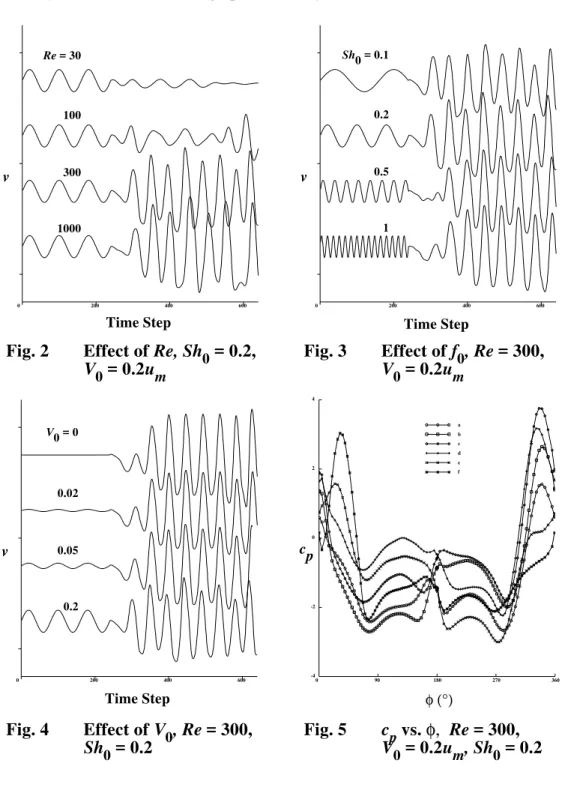
Figure 2 shows values of the cross-wise, v-velocity at the upstream monitor point P [Fig. 1] at Re = umd/ν values of 30, 100, 300 and 1000.
Figure 3 is a similar plot at various applied frequencies, corresponding to in-itial Strouhal numbers, Sh0 = of 0.1, 0.2, 0.5 and 1, at Re = 300. Figure 4 shows the influence of the amplitude of the initially applied disturbance; Val-ues are shown for V0 = 0, 0.02um, 0.05um, and 0.2um, where um is the bulk
velocity in the minimum cross-section (Sh0 = 0.2, Re = 300). Tb = 1tXt
n=1
Figure 5 shows an example of the behaviour of the instantaneous pres-sure coefficient, cp, defined as,
(4)
where p−(0), is the time-average pressure at φ = 0°.
c
p ≡ 1− p(0) 1− p(φ) 2ρu2m 0 200 400 600 Sh0 = 0.1 0.2 0.5 1 v Time Step 0 200 400 600 V0 = 0 0.02 0.05 0.2 v Time StepFig. 2 Effect of Re, Sh0 = 0.2, V0 = 0.2um Fig. 3 Effect of f0, Re = 300, V0 = 0.2um Fig. 4 Effect of V0, Re = 300, Sh0 = 0.2 0 200 400 600 Re = 30 100 300 1000 v Time Step Fig. 5 cp vs. φ, Re = 300, V0 = 0.2um, Sh0 = 0.2 -4 -2 0 2 4 0 90 180 270 360 a b c d e f cp φ (°)
Fig. 6 Stream-lines, Re = 300. (a) G H E B (b) (c) (f) (e) (d)
Table 1 Summary of results, stimulated response, Sh
0 = 0.2, V0 = 0.2um
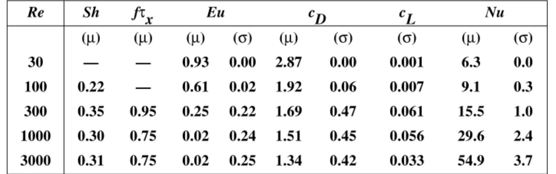
Table 2 Summary of results, spontaneous response, no lateral feedback
Figure 6 shows a sequence of six plots of stream-lines, illustrating the time-dependent flow patterns in the central zone B-G-H-E [Fig. 1] over one complete cycle, at Re = 300. Tables 1 and 2 are summaries of results for stimulated and spontaneous behaviour, respectively. All values are averaged over the last half of each simulation. The final frequency, f, is calculated from the v-velocity at monitor-point Q [Fig. 1]. The quantity, fτx, is that fraction of a cycle by which the upstream transient leads the value at the sub-sequent row, being computed from the v-values at the two monitor points P and Q.
Eu are computed as the mean pressure difference between two offset
rows normalised with respect to ½ρum2 Both the time-average value, µ, and
the sample standard deviation, σ are given in Tables 1 and 2. Lift and drag coefficients, cL and cD are defined as the net force per unit projected area, again normalised with respect to ½ρum2, while Nu is defined by,
(5)
where q is the constant wall heat flux, Tw is the wall temperature (around cylinders B-E) and the reference temperature, Tf , is taken to be the time-average bulk temperature in the upstream inter-tube space (mid-way between
A and B). Re Sh fτx Eu cD cL Nu (µ) (µ) (µ) (σ) (µ) (σ) (σ) (µ) (σ) 30 — — 0.92 0.06 2.88 0.05 0.017 6.4 0.1 100 0.27 0.73 0.57 0.06 1.88 0.17 0.047 8.9 0.3 300 0.35 0.89 0.37 0.18 1.73 0.31 0.062 15.5 1.1 1000 0.31 0.76 0.25 0.19 1.61 0.32 0.050 30.0 1.9 3000 0.26 0.82 0.16 0.20 1.32 0.33 0.027 56.6 2.9 Re Sh fτx Eu cD cL Nu (µ) (µ) (µ) (σ) (µ) (σ) (σ) (µ) (σ) 30 — — 0.93 0.00 2.87 0.00 0.001 6.3 0.0 100 0.22 — 0.61 0.02 1.92 0.06 0.007 9.1 0.3 300 0.35 0.95 0.25 0.22 1.69 0.47 0.061 15.5 1.0 1000 0.30 0.75 0.02 0.24 1.51 0.45 0.056 29.6 2.4 3000 0.31 0.75 0.02 0.25 1.34 0.42 0.033 54.9 3.7 Nu = πqd kZ π 0 Tw−Tf ° ± dφ
3 DISCUSSION
3.1 Independence of solution
Inspection of the monitor-point v-values in Fig. 2 shows that at Re = 30, the disturbance is damped out. For Re = 100, the transient maintains itself as is just apparent from the end of the trace in Fig. 2 (N.B. the downstream tran-sient leads by a further 240 time steps). As Re is increased the amplitude of the v-fluctuations increases to around 0.5um at Re = 300. At sufficient Re, a definite ‘transistor’ or ‘triode’-like effect was observed, whereby small lat-eral perturbations are amplified under the action of the main flow so the downstream oscillations are clearly larger than upstream values. By progres-sively back-substituting these downstream values, a stable periodic behav-iour is eventually established.
Figures 3 and 4 show the transient to be relatively unaffected by either the frequency, f0, or the magnitude, V0, of the initially applied disturbance, over a wide range. Note that the oscillations also arose spontaneously with
V0 = 0. Furthermore, spontaneous oscillations arose regardless of whether or
not the explicit lateral substitution mechanism, described above, was present. Although the ability to achieve vortex-shedding independently is highly en-couraging, the use of an external disturbance combined with a (lateral) feed-back mechanism is in some ways preferable: In the absence of an explicit lateral momentum boundary condition, it was found the flow would wander, resulting in a residual drift at low Re, while at higher Re, overall stability was difficult to control. For other geometries [7], the explicit back-substitution method proved to be the only way to induce transient behaviour. Note that the flow is fundamentally sensitive to span-wise disturbances (applied later-ally), much more so than to, say, fluctuations in u or v applied across the inlet
A-F.
The fluctuating u-velocity component, oscillates at 2f (due to the fact that it is the magnitude of the cross-wise v-fluctuations that influence the stream-wise velocity). These smaller u-velocity fluctuations are still signifi-cant, and influence the pressure trace. In contrast to v-fluctuations, the mag-nitude of the stream-wise u-fluctuations tends to increase with Re, becoming unstable and erratic. This is also especially true for the monitor-point pres-sure fluctuations.
The downstream pressure boundary condition, though approximate, ap-pears reasonable. Some distortion of the pressure field was observed (due to the concave shape of velocity profile near the the walls); however this was localised and should not affect the results. Some additional distortion due to the fact that curvature and divergence effects at the inlet were not accounted for was also apparent. It is interesting to note that, in spite of the non-orthogonal grid, transient behaviour proved much easier to generate here than for the case of flow in an in-line tube bank [7].
3.2 Description of flow field phenomena
Figure 6 shows a sequence of six sets of stream-lines for Re = 300. It can be seen that (a) A clockwise vortex has developed at the upper rear-side of upstream cylinder G. Below and downstream of this first vortex, a second counter-clockwise vortex can also be seen. (b) The clockwise vortex grows, in the presence of the favourable shear-layer, tending to increase angular mo-mentum. (c) This increases the size of the vortex, and displaces it back into the wake, to the rear of cylinder G. As the vortex moves across the centre-line, it encounters an adverse shear-layer (on the under-side of the cylinder) entraining it, and decreasing angular momentum. This results in a region of counter-clockwise vorticity being created between the vortex and the main stream. (d) The clockwise vortex is now displaced downstream, and the new counter-clockwise vortex begins to grow behind the rear-lower side of the cylinder. The (clockwise) vortex moves with the main flow and (e) is de-stroyed as it passes through the minimum cross-section of the subsequent row B-E. By (f) the cycle is complete. Owing to alternate quantities of clockwise and counter-clockwise momentum being imparted, the wake is ‘S’-shaped, and switches from side-to-side, in a sinuous fashion. The flow bifurcates at a point towards the front of the downstream cylinder H, the lo-cation of which moves as the stream sticks to alternate sides of the cylinder resulting in a ‘Coanda-like’ effect.
Flow-fields were found to be qualitatively similar at all Re: Stream-line plots were alike over a wide Re range, and only minor differences were noted regarding the size of vortices, number present, residence time and so forth. Comparison of the animation sequences of these results with the 16 mm cine-film of Weaver and Abd-Rabbo [3] revealed the numerical work to be physi-cally realistic, except that the experimentally observed vortices may possibly survive longer than is apparent from the data of Fig. 6, where they are de-stroyed as soon as they pass through the minimum cross-section of the subse-quent row. The reader will note that the stream-lines shown in of Fig. 6 were generated using a finite-volume solution of the stream-function vorticity equation [17]; non-iterative schemes were found to generate unrealistic re-sults due to the multiply-connected geometry.
Observed pressure fields were complex [17] with a maximum occurring near the bifurcation point, minima occurring at the sides of the cylinder (around φ = 90°), and multiple extrema occurring in the inter-tube space. Figure 5 shows the pressure coefficient cp as function of the angle, φ, from the leading edge of the cylinder (the same sequence shown in Fig. 6). A pressure rise is associated with the establishment of the attachment point at one or other side of the front of the cylinder (maxima rise and decay on op-posite side of each cylinder in an alternate fashion). The pressure minima, at the sides of the cylinder, are also transient. It can be seen that significant fluctuations in cp are observed around the entire periphery of the cylinder. Some slight discontinuities are apparent at the leading and trailing edges, due to the presence of ‘special-points’ in the grid, in these regions [see Fig. 1].
The presence of an overall favourable pressure gradient in the stream-wise direction would tend to impede vortex formation, suppressing such phe-nomena to higher Re in tube banks than in flow past single cylinders. It is also possible that the pressure field could assist the transient flow process:
For the simple case of potential flow [17, 18], the pressure is high at φ = 0° and 180°, and low at the sides, φ = ±90° of the cylinder. Thus a saddle-point exists in the the region corresponding to where the wake passes through the next (offset) row. This favourable lateral pressure gradient could give rise to a state of meta-stable equilibrium, assisting any wake-switching tendencies in the real situation.
3.3 Quantitative aspects
It can be seen, from Tables 1 and 2, that Sh were in the range 0.22 to 0.35, the mean value being around 0.3. Zukauskas et al. [19] suggest these to be of the order of 0.34, so numerically-obtained Sh are consistent with experimental values. Comparison of Tables 1 and 2 also shows broad agreement of Sh values for externally-induced and self-induced cases.
As Re increases the mean value of Eu decreases, while the periodic com-ponent becomes substantially larger. At high Re, the fluctuating comcom-ponent of the pressure field is very large compared to the steady-state value, affect-ing both Eu and cD which become erratic. On the other hand, cL oscillates in a sinusoidal-like manner. Time-average and fluctuating components of Nu increase with Re, however the latter is a much smaller fraction of the mean value than was observed for Eu or cD, as indicated by the ratio σ/µ. Inspec-tion of Tables 1 and 2 reveals Nu agreement to be much better than Eu values when comparing the cases of stimulated and spontaneous vortex-shedding
Because of the length of time required to make the numerical calcula-tions, only a few cycles could be considered in this study. Quantitative meas-ures of performance should therefore be considered as being only approxi-mate; many more cycles being required for precise figures. While boundary conditions and other factors (such as the assumption that the oscillations are in-phase in the cross-wise direction) may have affected some aspects of the transient process, it is maintained that the results are, for the most part, based on reasonable assumptions.
4 CONCLUSIONS
Staggered tube banks exhibit unstable behaviour for Re = 100. Below this value, externally applied oscillations die out, while above it they are am-plified. Alternate vortex shedding and wake-switching effects were ob-served. These were shown to be essentially independent of the applied signal over a wide range of applied amplitude and frequency. It was shown that the transients could also develop spontaneously. There is a large impact of the transient nature of the motion on the value of pressure-related quantities, such as cp and Eu. Sh values obtained using these calculations were found to be in reasonable agreement with experimentally obtained data.
NOMENCLATURE
aP, aW, aE, aS, aN, aT Linking coefficients in finite-volume equations
cD Drag coefficient
cL Lift coefficient
cf Skin friction coefficient
cp Pressure coefficient, specific heat
d Diameter
Eu Euler number
f, f0 Frequency, initial frequency
g Square of Jacobian, 1/det gij
gij Contravariant metric tensor
k Thermal conductivity
Nu
Overall Nusselt number
p, p− Pressure, mean pressure
P, Q Source terms in grid generation equations
q Heat flux
r
→ Position vector
Re Reynolds number
S Source term in finite-volume equations
Sh, Sh0 Strouhal number, initial Strouhal number
t Time
T−b Time-average bulk temperature
Tf Reference temperature
Tw Wall temperature
u, v Stream-wise, cross-wise velocity
um Bulk velocity
V0 Peak applied disturbance
x, y Stream-wise, cross-wise displacement
µ Sample mean
ρ Density
σ Population standard deviation
τw Shear stress
τx, τy Stream-wise, cross-wise phase
φ Angle from front of cylinder
φP, φW, φE, φS, φN, φT Values of variable φ in finite-volume equations
REFERENCES
1. OWEN, P.R. - Buffeting Excitation of Boiler Tube Vibration. Journal of Mechanical Engineering Science, Vol. 7, pp. 431-439, 1965.
2. WALLIS, R. PENDENNIS - Photographic Study of Fluid Flow between Banks of Tubes. Engineering, Vol. 148, pp. 423-425. (also Proceedings of the IMechE, Vol. 142, pp.379-387, 1939).
3. WEAVER, D.S., and ABD-RABBO, A. - Flow Visualisation in In-Line and Staggered Tube Banks. 16mm cine film. Department of Mechani-cal Engineering, McMaster University. 1984.
4. ABD-RABBO, A. and WEAVER, D.S. - A Flow Visualisation Study of Flow Development in a Staggered Tube Array. Journal of Sound and Vi-bration, Vol. 106 (2), pp. 241-256, 1986.
5. PAÏDOUSSIS, M.P. - A Review of Flow-induced Vibrations in Reactors and Reactor Components. Nuclear Engineering and Design, Vol. 74, pp. 31-60, 1982.
6. STUHMILLAR, J.H., CHILUKURI, R., MASIELLO, P.J., CHAN., R.K.C., YU, J.H.Y., and HO., K.H.H. - Prediction of Localized Flow Velocities and Turbulence in a PWR Steam Generator. Project S310-14, Final Report, Electric Power Research Institute, Palo Alto, California. (EPRI NP-5555), 1988.
7. BEALE, S.B., and SPALDING, D.B. - Paper Submitted to the IMechE Conference on Engineering Applications of Computational Fluid Dy-namics, London, 1993.
8. THOMPSON, J.F., WARSI, Z.U.A., and MASTIN, C.W. - Numerical Grid Generation, Foundations and Applications. Elsevier, New York and Amsterdam. 1985.
9. PATANKAR, S.V., and SPALDING, D.B. - A Calculation Procedure for Heat, Mass, and Momentum Transfer in Three-dimensional Parabolic Flows. International Journal of Heat and Mass Transfer, Vol. 15, pp. 1787-1806, 1972.
10. SPALDING, D.B. - A Novel Finite-difference Formulation for Differen-tial Expressions involving Both First and Second Derivatives. Interna-tional Journal for Numerical Methods in Engineering, Vol. 4, pp. 551-559, 1972.
11. CARETTO, L.S., GOSMAN, A.D., PATANKAR, S.V., and SPAL-DING, D.B. - Two Calculation Procedures for Steady, Three-dimensional Flows with Recirculation. Proceedings of the 3rd Interna-tional Conference on Numerical Methods in Fluid Mechanics. Springer Verlag - Lecture Notes in Physics, Vol. 2, No. 19, pp. 60-68, 1973. 12. PATANKAR, S.V. - Numerical Heat Transfer and Fluid Flow.
Hemi-sphere, New York, 1980.
13. SPALDING, D.B. - Mathematical Modelling of Fluid-mechanics, Heat-transfer and Chemical-reaction Processes: A Lecture Course. HTS/80/1, Computational Fluid Dynamics Unit, Imperial College, University of London. 1980.
14. SPALDING, D.B. - Four Lectures on the PHOENICS Code. CFD/82/5, Computational Fluid Dynamics Unit, Imperial College, University of London, 1982.
15. SPALDING, D.B. - PHOENICS 1984 - A dimensional Multi-phase General-purpose Computer Simulator for Fluid Flow, Heat Trans-fer and Combustion. CFD/84/18, Computational Fluid Dynamics Unit, Imperial College, University of London, 1984.
16. WATSON, V., WALATKA, P.P., BANCROFT, G., PLESSEL T., and MERRRITT, F. - Visualisation of Fluid Dynamics at NASA Ames. Computing Systems in Engineering, Vol. 1, Nos. 2-4, pp. 333-340, 1990. 17. BEALE, S.B. - Fluid Flow and Heat Transfer in Tube Banks. Ph.D.
Thesis, Imperial College, University of London, 1993.
18. BEALE, S.B. - Potential Flow in In-Line and Staggered Tube Banks. NRC Technical Report IME-CRE-TR-006. National Research Council of Canada, 1993.
19. ZUKAUSKAS, A.A, ULINSKAS, R.V., and KATINAS, V. - Fluid Dy-namics and Flow-induced Vibrations of Tube Banks. Hemisphere, New York. (English-edition editor, J. Karni), 1988.