Applications of network optimization

July 1992 WP #3458 Ravindra K. Ahuja* Thomas L. Magnanti*

James B. Orlin* M.R. Reddy

* see page bottom for complete address

Ravindra K. Ahuja

Department of Industrial & Management Engineering Indian Institute of Technology

Kanpur - 208 016, INDIA Thomas L. Magnanti

Sloan School of Management

Massachusetts Institute of Technology Cambridge, MA 02139

James B. Orlin

Sloan School of Management

Massachusetts Institute of Technology Cambridge, MA 01239

MR. Reddy

Department of Industrial & Management Engineering Indian Institute of Technology

Kanpur - 208 016, INDIA

Ravindra K. Ahuja, Thomas L. Magnanti, James B. Orlin, and M. R. Reddy

ABSTRACT

Network optimization has always been a core problem domain in operations research, as well as in computer science, applied mathematics, and many fields of engineering and management. Network optimization problems arise in a variety of situations, and often in situations that apparently are quite unrelated to networks. These applications are scattered throughout the literature and until recently no single paper, book, or any other reference, summarized these applications. Consequently, the research and practitioner community has not fully appreciated the richness of these applications. This paper attempts to partially satisfy this important need by presenting a collection of applications of the following fundamental network optimization problems: the shortest path problem, the maximum flow problem, the minimum cost flow problem, assignment and matching problems, and the minimum spanning tree problem. We describe 25 applications of these problems and provide references for more than 100 additional applications. This paper is

intended to provide an appreciation for the pervasiveness of network optimization problems. We hope that this paper will stimulate researchers and practitioners to model more decisions problems within the framework of network optimization.

1. INTRODUCTION

Everywhere we look in our daily lives, networks are apparent. Electrical and power networks bring lighting and entertainment into our homes. Telephone networks permit us to communicate with each other almost effortlessly within our local communities and across regional and international borders. National highway systems, rail networks, and airline service networks provide us with the means to cross great geographical distances to accomplish our work, to see our loved ones, and to visit new places and enjoy new experiences. Manufacturing and distribution networks give us access to life's essential foodstock and to consumer products. And computer networks, such as airline reservation systems, have changed the way we share information and conduct our business and personal lives. In all of these problem domains, and in many more, we wish to send some flow (electricity, a consumer product, a person or a vehicle, a message) from one point to another in an underlying physical network, and to do so as efficiently as possible, both to provide good service to the users of the network and to use the underlying (and typically expensive) transmission facilities effectively. These problems constitute the domain of network optimization problems.

Network optimization problems in many other settings, do not correspond to any direct physical systems. For example, sometimes the nodes and arcs have a temporal dimension that models activities that take place over time. Many scheduling applications have this flavor. Network optimization problems also arise in surprising ways for problems that on the surface might not appear to involve networks at all. In any event, networks model a variety of problems in project, machine and crew scheduling; location and layout; warehousing and distribution; production planning and control; and social, medical, and defense contexts; and in the physical and life sciences. The operations research, applied mathematics, computer science, and engineering communitites have made many successes on this front, and a wide variety of practical problems can be formulated and solved as network optimization problems. These applications, however, are scattered throughout the literature, and until recently no single paper, book or any other reference summarized these applications. Consequently, the research and practitioner communities lacked awareness of these applications. This paper helps to fill this need by describing 25 applications and providing references for over 100 additional applications of the following fundamental network optimization problems: (1) the shortest path problem; (2) the maximum flow problem; (3) the minimum cost flow problem; (4) assignment and matching problems; and (5) the minimum spanning tree problem. We have selected these problem categories on account of their importance to the operations research community. The applications for these problems can be partitioned into two category: (i) optimization problems that are transformable into one of the network optimization problems cited in this list; and (ii) optimization problems that contain embedded network structure and are solvable by solving a sequence of network optimization problems. We have limited the scope of our discussion in this paper to applications in the first category. The 25 applications described in this paper arise in the following domains:

I. Approximating piecewise linear functions. 2. DNA sequence alignment

3. Production planning problems. 4. System of difference constraints. 5. Telephone operator scheduling. 6. Matrix rounding problem.

7 Baseball elimination problem. 8. Open pit mining.

9. Scheduling on uniform parallel machines. 10. Tanker scheduling problem.

11. Leveling mountainous terrain

12. Reconstructing the left ventricle from X-ray projections. 13. Optimal loading of a hopping airplane.

14. Directed Chinese postman problem. 15. Models for building evacuation. 16. Personell assignment.

17. Paring stereo speakers. 18. Locating objects in space. 19. Matching moving objects. 20. Determing chemical bonds. 21. Designing physical systems.

22. Measuring homogeneity of bimetallic objects. 23. Reducing data storage.

24. All pairs minimax path problem. 25. Cluster analysis.

The applications described in this paper are drawn from important operations research, computer science and applied mathematics journals. The integer programming bibliographies by Kastning [1976], Hausman [1978] and Von Randow [1982, 1985] have helped us to identify these applications. We have excerped these applications from our fortcoming book, "Network Flows: Theory, Algorithms, and Applications," written by the first three authors of this paper. This book describes a total of 150 applications of the network optimization problems and provides many more references for the shortest paths, maximum flows, minimum cost flows, assignments and matchings, minimum spanning trees, convex cost flows, generalized flows, and multicommodity flows.

2. PRELIMINARIES

In this section, we present some basic notation and definitions of graph theory that we use in this paper. We also present a mathematical programming formulation of the minimum cost flow problem, which: is the core network optimization problem studied in this paper.

Let G = (N, A) be a directed network defined by a set N of n nodes, and a set A of m directed arcs. Each arc (i, j) E A has an associated cost cij per unit flow on that arc. We assume that the flow cost varies linearly with the amount of flow. Each arc (i, j) E A also has a capacity uij denoting the maximum amount that can flow on the arc, and a lower bound lij denoting the minimum amount that must flow on the arc. We associate with each node i e N an integer number b(i) representing its supply/demand. If b(i) > 0, then node i is a supply node; if b(i) < 0, then node i is a demand node; and if b(i) = 0, then node i is a transshipment node.

The minimum cost flow problem is easy to state: we wish to determine a least cost shipment of a commodity through a network that will satisfy the flow demands at the demand nodes from available supplies at other nodes. The decision variables in the minimum cost flow problem are arc flows and we represent the flow on an arc (i, j) e A by xij. The minimum cost flow problem is an optimization model formulated as follows:

Minimize I cij xij (la)

(i, j) A subject to

X

X

j : (i, j) e A} (j: (j i) E Al

lij < xij < uij, for all (i, j) E A, (Ic)

with data satisfying the feasibility condition i=1b(i) = 0 (that is, the total supply must equal the total

demand). We refer to the constraints in (Ib) as the mass balance constraints. The mass balance constraints state that the outflow into each node minus its inflow must equal the supply/demand of the node. The flow must also satisfy the lower bound and capacity constraints (c) which we refer to as the flow bound constraints. The flow bounds typically model physical capacities or restrictions imposed upon the flows' operating ranges. In most applications, the lower bounds on arc flows are zero; therefore, if we do not state lower bounds explicitly, we assume they have value zero.

We now collect together several basic definitions and describe some notation. A path in G = (N, A) is a sequence of distinct nodes and arcs i1, (i1, i2), i2, (i2, i3), i3... ( irl, i), ir satisfying the property

that either (ik, ik+1) e A or (ik+l, ik) e A for each k = 1 . . ., r-1. For simplicity of notation, we often refer to a path as a sequence of nodes i - i2 - ... -ik when its arcs are apparent from the problem

context. A directed path is defined similarly except that for any two consecutive nodes ik and ik+l on the path, the path must contain the arc (ik, ik+l). A directed cycle is a directed path together with the arc (ir il), and a cycle is a path together with the arc (ir, il) or (i1 , i).

A graph G' = (N', A) is a subgraph of G = (N, A) if N' N and A' A. A graph G' = (N', A') is a spanning subgraph of G = (N, A) if N' = N and A' C A. Two nodes i and j are said to be connected if the graph contains at least one undirected path from i to j. A graph is said to be connected if all pairs of its nodes are connected; otherwise, it is disconnected. The connected subgraphs of a graph are called its components. A tree is a connected graph that contains no cycle. A subgraph T is a spanning tree of G if T is a tree of G containing all its nodes. A cut of G is any set Q Q A with the property that the graph G' = (N, A-Q) is disconnected, and no subset of Q has this property. A cut partitions the graph into two sets of nodes, X and N-X. We shall sometimes represent the cut Q as the node partition X, N-X]. A cut [X, N-X] is an s-t cut for two specially designated nodes s and t if s e X and t e N-X.

3. SHORTEST PATH PROBLEM

The shortest path problem is among the simplest network optimization problems. In this problem, we wish to find a path of minimum cost (length) from a specified source node s to another specified sink node t assuming that each arc (i, j) e A has an associated cost (or length) cij. In the formulation of the minimum cost flow problem given in (1), if we set b(s) = 1, b(t) = -1, and b(i) = 0 for all other nodes, then the solution to this problem will send one unit of flow from node s to node t along the shortest path. If we want to determine shortest paths from the source node s to every other node in the network, then in the minimum cost flow problem, we set b(s) = (n-1) and b(i) = -1 for all other nodes. We can set each arc capacity uij to any number larger than (n-l). The minimum cost flow solution would then send one unit flow from node s to every other node i along a shortest path.

Shortest path problems are alluring to both researchers and to practitioners for several reasons: (i) they arise frequently in practice since in a wide variety of application settings we wish to send some material (for example, a computer data packet, a telephone call, a vehicle) between two specified points in a network as quickly, as cheaply, or as reliably as possible; (ii) they are easy to solve efficiently; (iii) as the simplest network models, they capture many of the most salient core ingredients of network flows and so they provide both a benchmark and a point of departure for studying more complex network models; and (iv) they arise frequently as subproblems when solving many combinatorial and network optimization problems. In this section, we describe a few applications of the shortest path problem that are indicative of its range of applications. The applications arise in applied mathemetics, biology, computer science, production planning, and work force scheduling. We conclude the section by producing references for many additional applications in a wide variety of fields.

Application 1. Approximating Piecewise Linear Functions (Imai and Iri [19861)

Numerous applications encountered within many different scientific fields use piecewise linear functions. On several occasions, because these functions contain a large number of breakpoints, they are expensive to store and to manipulate (for example, even to evaluate). In these situations, it might be advantageous to replace the piecewise linear function by another approximating function that uses fewer breakpoints. By approximating the function, we will generally be able to save on storage space and on the cost of using the function; we will, however, incur a cost because of the inaccuracy of the approximating function. In making the approximation, we would like to make the best possible tradeoff between these conflicting costs and benefits.

Let f(x) be a piecewise linear function of a scalar x. We represent the function in the two-dimensional plane: it passes through n points a, = (xl,y1), a2= (x2,y2),..., an= (xn,yn). Suppose that we

have ordered :es ,oints so that x < x2< --. < x . We assume that the function varies linearly between

every two cons*dutive points xiand xi+1. We consider situations in which n is very large and for practical

reasons we wish to approximate the function fl(x) by another function f2(x) that passes through only a

subset of the points a₁, a₂, ..., an (including a and an). As an example, consider Figure (a): in this figure, we have approximated a function fl(x) passing through 10 points by a function f2(x) (drawn with

I

f(x)

(a) (b)

Figure 1. Approximating precise linear functions.

(a) Approximating a function fl(x) passing through 10 points by a function f2(x) passing through only 5 points.

(b) Corresponding shortest path problem.

This approximation results in a savings in storage space and in the use of the function. For purposes of illustration, assume that we can measure these costs by a per unit cost a associated with any single interval used in the approximation (which is defined by two points ai and aj). As we have noted, the

approximation also introduces errors which have an associated penalty. We assume that the error of an approximation is proportional to the sum of the squared errors between the actual data points and the estimated points, i.e., the penalty is iPl [fl(xi) - f2(xi)]2for some constant 3. Our decision problem is

to identify the subset of points to be used to define the approximation function f2(x) so we incur the

minimum total cost as measured by the sum of the cost of storing and the cost of the errors imposed by the approximation.

We formulate this problem as a shortest path problem on a network G with n nodes, numbered 1 through n, as follows. The network contains an arc (i, j) for each pair of nodes i and j. Figure (b) gives an example of the network with n = 4 nodes. The arc (i, j) in this network signifies that we approximate the linear segments of the function fl (x) between the points ai, ai+1,... aj by one linear segment joining

the points aiand aj. The cost cij of the arc (i, j) has two components: the storage cost a and the penalty

associated with approximating all the points between aiand aj by the corresponding points lying on the line

joining ai and aj. In the interval [xi, xj], the approximating function is f2(x) = (x xi)(fl(xj) f(xi)l/(xj

-xi) and so the total cost in this interval is

Cij = a + =i (fl(xk) - f2(xk))2 1.

Each directed path from node I to node n in G corresponds to a function f2(x), and the cost of this path

equals the total cost for storing this function and for using it to approximate the original function. For example, the path 1-3-4 corresponds to the function f2(x) passing through the points al, a3and a4. As a

consequence of these observations, we see that the shortest path from node 1 to node n specifies the optimal set of points needed to define the approximating function f2(x).

I I I I I 11112 1 -3V Y?

7

Application 2. DNA Sequence Alignment (Waterman [1988])

Scientists model strands of DNA as a sequence of letters drawn from the alphabet A, C, G, T) Given two sequences of letters, say B = blb2... bp and D = dld2... dq of possibly different lengths, molecular

biologists are interested in determining how similar or dissimilar these sequences are to each other. (These sequences are subsequences of a genome and typically contain several thousand letters.) A natural way of measuring the dissimilarity between the two sequences B and D is to determine the minimum "cost" required to transform sequence B into sequence D. To transform B into D, we can perform the following operations: (i) insert an element in B (at any place in the sequence) at a "cost" of a units; (ii) delete an element from B (at any place in the sequence) at a "cost" of 3 units; and (iii) mutate an element biinto an

element dj at a "cost" of g(bi, dj) units. Needless to say, it is possible to transform the sequence B into the

sequence D in many ways and so identifying a minimum cost transformation is a nontrivial task. We show how we can solve this problem using dynamic programming, which we can also view as solving a shortest path problem on an appropriately defined network.

Suppose that we conceive of the process of transforming the sequence B into the sequence D as follows. First, add or delete elements from the sequence B so that the modified sequence, say B', has the same number of elements as D. Next "align" the sequences B' and D to create a one-to-one alignment between their elements. Finally, mutate the elements in the sequence B' so that this sequence becomes identical with the sequence D. As an example, suppose that we wish to transform the sequence B = AGTT into the sequence D = CTAGC. One possible transformation is to delete one of the elements T from B and add two new elements at the beginning, giving the sequence B' = $AGT (we denote any new element by a placeholder and later assign a letter to this placeholder). We then align B' with D, as shown in Figure 2, and mutate the element T into C so that the sequences become identical. Notice that because we are free to assign values to the newly added elements, they do not incur any mutation cost. The cost of this transformation is 5+2a+g(T,C).

B'= @AGT C TAGC

D =C T AGC C TAGC

Figure 2. Transforming the sequence B into the sequence D.

We now describe a dynamic programming formulation of this problem. Let f(i, j) denote the minimum cost of transforming the subsequence blb2...bi into the subsequence dld2...dj. We are interested in the

value f(p,q), which is the minimum cost of transforming B into D. To determine f(p,q), we will determine f(ij) for all i = 0, 1, ..., p, and for all j = 0 , ..., q. We can determine these intermediate quantities f(i, j) using the following recursive relationships:

f(i,0) = i for all i; (2a)

f(0,j) = a j for all j; and (2b)

We now justify this recursion. The cost of transforming a sequence of i elements into a null sequence is the cost of deleting i elements. The cost of transforming a null sequence into a sequence of j elements is the cost of adding j elements. Next consider f(ij). Let B' denote the optimal aligned sequence of B (i.e., the sequence just before we create the mutation of B' to transform it into D). At this point, B' satisfies exactly one of the following three cases:

Case 1. B' contains the letter biwhich is aligned with the letter dj of D (as shown in Figure 3(a)). In

this case, f(ij) equals the optimal cost of transforming the subsequence blb2...bi l into d1d2...dj 1and the

cost of transforming the element biinto dj. Therefore, f(ij) = f(i- 1, j- 1) + g(bi, dj).

Case 2. B' contains the letter biwhich is not aligned with the letter d (as shown in Figure 3(b)). In this

case, biis to the left of dj and so a newly added element must be aligned with bj. In this case, f(ij) equals

the optimal cost of transforming the subsequence blb2...bi into dld2... dj l plus the cost of adding a new

element to B. Therefore, f(i,j) = f(ij-1) + a.

Case 3. B' does not contains the letter bi. In this case, we must have deleted bifrom B and so the

optimal cost of the transformation equals the cost of deleting this element and transforming the remaining sequence into D. Therefore, f(ij) = f(i- j) + 3.

B' D

d,

d

...

dii

1

Figure 3. Explaining the dynamic programming recursion.

The preceding discussion justifies the recursive relationships specified in (2). We can use these relationships to compute f(i,j) for increasing values of i and, for a fixed value of i, for increasing values of j. This method allows us to compute f(p, q) in O(pq) time, that is time proportioned to the product of the number of elements in the two sequences.

We can alternatively formulate the DNA sequence alignment problem as a shortest path problem. In Figure 4, we show the shortest path network for this formulation for a situation with p = 3 and q = 3. For simplicity, in this network we let gij denote g(bi, dj). We can establish the correctness of this formulation

by applying an induction argument based upon the induction hypothesis that the shortest path length from node 00 to node i equals f(i,j). The shortest path from node 00 to node i must contain one of the following arcs as the last arc in the path: (i) arc (i-lj-l, ii); (ii) arc (ij1, i), or (iii) arc (i-lj, ii). In these three cases, the lengths of these paths will be f(i-l j-l) + g(bi, dj), f(i,j-l)+ a, and f(i-1, j) + 3. Clearly,

9

the shortest path length f(i,j) will equal the minimum of these three numbers, which is consistent with the dynamic programming relationships stated in (2).

Figure 4. Sequence alignment problem as a shortest path problem.

This application shows a relationship between shortest paths and dynamic programming. We have seen how to solve the DNA sequence alignment problem through the dynamic programming recursion or by formulating and solving it as a shortest path problem on an acyclic network. The recursion we use to solve the dynamic programming problem is just a special implementation of one of the standard algorithms for solving shortest path problems on acyclic networks. This observation provides us with a concrete illustration of the meta statement that "(deterministic) dynamic programming is a special case of the shortest path problem". Accordingly, shortest path problems model the enormous range of applications in many disciplines that are solvable by dynamic programming.

Application 3. Production Planning Problems ([Veinott and Wagner [1962],

Zangwill [19691, Evans [1977])

Many optimization problems in production and inventory planning are network optimization models. All of these models address a basic economic order quantity issue: when we plan a production run of any particular product, how much should we produce? Producing in large quantities reduces the time and cost required to set up equipment for the individual production runs; on the other hand, producing in large quantities also means that we will carry many Hrems in inventory awaiu ng purchase by customers. The economic order quantity strikes a balance betwernr the set up and invens ry costs to find the production plan that achieves the lowest overall costs. The modes that we consider in this section all attempt to balance the production and inventory carrying costs while meeting known demands that vary throughout a given planning horizon. We study one of the simplest models: a single product, single stage model with concave costs and backordering.

In this model, we assume that the production cost in each period is a concave function of the level of production. In practice, the production xj in the jth period frequently incurs a fixed cost Fj (independent of the level of production) and a per unit production cost cj. Therefore, for each period j, the production cost is 0 for xj = 0 and F + cj xj if xj > 0, which is a concave function of the production level xj. The production cost might also be concave due to other economies of scale in production. In this model, we also permit backordering, which implies that we might not fully satisfy the demand of any period from the production in that period or from current inventory, but could fulfill the demand from production in future periods. We assume that we do not lose any customer whose demand is not satisfied on time and who must wait until his

or her order materializes. Instead, we incur a penalty cost for backordering any item. We assume that the inventory carrying and backordering costs are linear, and that we have no capacity imposed upon production, inventory, or backordering volumes.

In this model, we wish to meet a prescribed demand dj for each of K periods j = 1, 2, ...,'K, by either producing an amount xj in period j, by drawing upon the inventory Ij.l carried from the previous period, and/or by backordering the item from the next period. Figure 5(a) shows the network for modeling this problem. The network has K+1 nodes: the jth node, for j = 1, 2, ..., K, represents the jLh planning period; node 0 represents the "source" of all production. The flow on the production arc (0, j) prescribes the production level xj in period j, and the flow on inventory carrying arc (j, j+1) prescribes the inventory level Ij

to be carried from period j to period j +1, and the flow Bj on the backordering arc (j, j- 1) represents the amount backordered from the next period.

The network flow problem in Figure 5(a) is a concave cost flow problem, because the cost of flow on every production arc is a concave function. The following well known result about the concave cost flow problems helps us to solve this problem: These problems always have an optimal spanning tree solution (see, for example, Ahuja, Magnanti and Orlin [19931). Figure 5(b) shows an instance of the spanning tree solution. This result implies the following property, known as the production property: In the optimal solution, each time we produce, we produce enough to meet the demand for an integral number of contiguous periods. Moreover, in no period do we both produce and carry inventory from the previous or next period.

Y it e n. ;e g d

11 K d, i=1 (a) - (b)

Figure 5. Production planning problem. (a) Underlying network.

(b) Graphical structure of a spanning tree solution.

The production property permits us to solve the production planning problem very efficiently as a shortest path problem on an auxiliary network G' defined as follows. The network G' consists of nodes 1 through K+1 and contains an arc (i, j) for every pair of nodes i and j with i < j. We set the cost of arc (i, j) equal to the sum of the production, inventory carrying and backorder carrying costs incurred in satisfying the demands of periods i, i+ l,..., j- by producing in some period k between i and j-1; we select this period k that gives the least possible cost. In other words, we vary k from i to j-1, and for each k, we compute the cost incurred in satisfying the demands of periods i through j-1 by the production in period k; the minimum of these values defines the cost of arc (i, j) in the auxiliary network G'. Observe that for every production schedule satisfying the production property, G' contains a directed path from node 1 to node K+1 with the

L - .- -... s>..a __I _A.- _ - L _ ._ __XI

saiic UUJV o cuve Iunuon val U, ian viLc-versa. i1Cnerere, we c an oUlin me U puimai prUaucuon ai;cuul; Uy

solving a shortest path problem.

Several variants of the production planning problem arise in practice. If we impose capacities on the production, inventory, or backordering arcs, then the production property does not hold and we can not formulate this problem as a shortest path problem. In this case, however, if the production cost in each

x I II

I

period is linear, then the problem becomes a minimum cost flow model. The minimum cost flow model also models multistage situations, where the product passes through a sequence of operations. We treat each production operation as a separate stage and require that the product pass through each of the stages before its production is complete. In a further multi-item generalization where the common manufacturing facilities are used to manufacture multiple products in multiple stages; this problem is a multicommodity flow problem. The references cited for this application describe these various generalizations.

Application 4. System of Difference Constraints (Bellman [19581)

In some linear programming applications, with constraints of the form Ax < b, the nxm constraint matrix A contains one +1 and one - in each row; all the other entries are zero. Suppose that the kthrow has a +1 entry in column k and a -1 entry in column ik; the entries in the vector b have arbitrary signs. This linear program defines the following set of m difference constraints in the n variables x = (x(l), x(2), x(n)):

x(Jk) - x(ik) < b(k), for each k=l,..., m. (3)

We wish to determine whether the system of difference constraints given by (3) has a feasible solution, and if so, we want to identify one. This model arises in a variety of applications; in the following application we describe the use of this model in the telephone operator scheduling, an additional application arises in the scaling of data (Orlin and Rothblum [1985]) and just-in-time scheduling (Elmaghraby [1978] and Levner and Nemirovsky [1991 ).

Each system of difference constraints has an associated graph G, which we call a constraint graph. The constraint graph has n nodes corresponding to the n variables and m arcs corresponding to the m difference constraints. We associate an arc (ik, jk) of length b(k) in G with the constraint x(jk) - x(ik) < b(k). As an example, consider the following system of constraints whose corresponding graph is shown in Figure 6(a).

x(3) - x(4) 5 5, (4a)

x(4) - x(1) < -10, (4b)

x(l) - x(3) ; 8, (4c)

x(2) - x(l) < - 1, (4d)

- %

(a) (b)

Figure 6. Graph corresponding to a system of difference constraints.

To model the problem use two well known results about shortest paths: (i) the optimality conditions for the shortest path distances d(.), in the network G = (N, A) satisfy the optimality criteria d(j) - d(i) < cij for all (i, j) E A; and (ii) the shortest path distances exist if and only if the network G does not contain a negative cycle (see Cormen, Leiserson, and Rivest [1990] and Ahuja, Magnanti, and Orlin [1993]). Notice the similarity between the difference inequalities (4) and the shortest path optimality conditions. The first result that the network for which (4) become the shortest path optimality conditions is given in Figure 6(a). The network shown in Figure 6(a) contains a negative cycle 1-2-3 of length -1, and the corresponding constraints (i.e., x(2) - x(l) < -11, x(3) - x(2) < 2 and x(1) - x(3) < 8) are inconsistent because summing these constraints yields 0 < -1. Therefore, we conclude that the system of difference constraints given by (4) has no feasible solution.

We can detect the presence of a negative cycle in a network by using a label correcting algorithm. Label correcting algorithms require that all the nodes in the network are reachable y a directed path from some node, which we use as the source node for the shortest path problem. To saLsfy this requirement, we introduce a new node s and join it to all the nodes in the network with arcs of zero cost. For our example, Figure 6(b) shows the modified network. Since all of the arcs incident to node s are directed out of this node, node s is not contained in any directed cycle and so the modification does not create any new directed cycles, and so does not introduce any cycles with negative costs. The label correcting algorithms either indicate the presence of a negative cycle or provide the shortest path distances. In the former case, the system of difference constraints has no solution, and in the latter case, the shortest path distances constitute a solution of (4).

Application S. Telephone Operator Scheduling (Bartholdi, Orlin and Ratliff [19801)

As an application of the system of difference constraints, consider the following telephone operator scheduling problem. A telephone company needs to schedule operators around the clock. Let b(i) for i = 0, 1, 2, ... , 23, denote the minimum number of operators needed for the ith hour of the day (here b(0) denotes number of operators required between midnight and I AM). Each telephone operator works in a shift of 8 consecutive hours and a shift can begin at any hour of the day. The telephone company wants to determine a "cyclic schedule" that repeats daily, i.e., the number of operators assigned to the shift starting at 6 AM and ending at 2 PM is the same for each day. The optimization problem requires that we identify the

fewest operators needed to satisfy the minimum operator requirement for each hour of the day. If we let yi denote the number of workers whose shift begins at the ith hour, then we can state the telephone operator scheduling problem as the following optimization model:

Minimize 1 23 (5a)

subject to

Yi-7 + Yi-6 + .. + Yi 2 b(i), for all i = 8 to 23, (5b)

Y17+i + --+ Y23 + YO +---+ i >b(i), for all i = O to 7, (5c)

Yi > 0 for all i = 0 to 23. (5d)

Notice that this linear program has a very special structure because the associated constraint matrix contains only O's and 's and the 's or O's in each row appear consecutively. In this application, we study a restricted version of the telephone operator scheduling problem: we wish to determine whether some feasible schedule uses p or fewer operators. We convert this restricted problem into a system of difference constraints by redefining the variables. Let x(O) = yo, x(l) = y + Yl, x(2) = y + yl + y2... , and x(23)

= Y +Y2 + -- +Y23 = P. Now notice that we can rewrite each constraint in (5b) as

x(i) - x(i-8) > b(i), for all i = 8 to 23, (6a)

and each constraints in (5c) as

x(23) - x(16+i) + x(i) = p - x(16-i) + x(i) > b(i), for all i = 0 to 7. (6b) Finally, the nonnegativity constraints (5d) become

x(i) - x(i - 1) > O. (6c)

By virtue of this transformation, we have reduced the restricted version of the telephone operator scheduling problem into a problem of finding a feasible solution of the system of difference constraints.

Additional Applications

Some additional applications of the shortest path problem include (1) knapsack problem (Fulkerson [19661); (2) tramp steamer problem (Lawler [19661); (3) allocating inspection effort on a production line (White [1969]); (4) reallocation of housing (Wright 19751); (5) assortment of steel beams (Frank [1965]); (6) compact book storage in libraries (Ravindran [19711); (7) concentrator location on a line (Balakrishnan, Magnanti and Wong 1989]); (8) manpower planning problem (Clark and Hasting [19771);

(9) equipment replacement (Veinott and Wagner [1962]); (10) determining minimum project duration

(Elmaghraby [1978]); (11) assembly line balancing (Gutjahr and Nemhauser 1964]); (12) optimal

improvement of transportation networks (Goldman and Nemhauser [19671); (13) machining process optimization (Szadkowski [1970]); (14) capacity expansion (Luss 19791); (15) routing in computer communication networks (Schwartz and Stem [(1980]); (16) scaling of matrices (Golitschek and Schneider

[1984]); (17) city traffic congestion (Zawack and Thompson [19871); (18) molecular confirmation (Dress and Havel [1988]); (19) order picking in an isle (Goetschalckx and Ratliff [1988]); and (20) robot design (Haymond, Thornton, and Warner [1988]. Shortest path problems often arise as important subroutines within algorithms for solving many different types of network optimization problems. These applications are too numerous to mention.

4. MAXIMUM FLOW PROBLEM

The maximum flow problem is in a sense a complementary model to the shortest path problem. The shortest path problem models situations in which flow incurs a cost, but is not restricted by any capacities;

in contrast, in the maximum flow problem flow incurs no costs, but is restricted by flow bounds. The maximum flow problem seeks a feasible solution, which sends the maximum amount of flow from a specified source node s to another specified sink node t. If we interpret uij as the maximum flow rate of arc (i, j), then the maximum flow problem identifies the maximum steady-state flow that the network can send from node s to node t per unit time. We can formulate this problem as a minimum cost flow problem in the following manner. We set b(i) = 0 for all i e N, cij = 0 for all (i, j) e A, and introduce an additional arc (t, s) with cost cts = -1 and flow bound uts = Co. Then the minimum cost flow solution maximizes the flow on arc (t, s); but since any flow on arc (t, s) must travel from node s to node t through the arcs in A (since each b(i) = 0), the solution to the minimum cost flow problem will maximize the flow from node s to node t in the original network.

The maximum flow problem arises in a wide variety of situations and in several forms. Examples of the maximum flow problem include determining the maximum steady state flow of (i) petroleum products in a pipeline network, (ii) cars in a road network; (iii) messages in a telecommunication network; and (iv) electricity in an electrical network. Sometimes the maximum flow problem occurs as a subproblem in the solution of more difficult network problems such as the minimum cost flow problem or the generalized flow problem. The maximum flow problem also arises in a number of combinatorial applications that on the surface might not appear to be maximum flow problems at all. In this section, we describe a few such applications.

Application 6. Matrix Rounding Problem (Bacharach [1966])

This matrix rounding application is concerned with consistent rounding of the elements, row sums, and column sums of a matrix. We are given a pxq matrix of real numbers D = (ddij, with row sums ai and column sums j. We can round any real number to the next smaller integer La] or to the next larger integer Fal and the decision to round up or down is entirely up to us. The matrix rounding problem requires that we round the matrix elements, and the row and column sums of the matrix so that the sum of the rounded elements in each row equals the rounded row sum, and the sum of the rounded elements in each column equals the rounded column sum. We refer to such a rounding as a consistent rounding.

We shall formulate this problem and some of the subsequent following applications as a problem known as a feasible flow problem. In the feasible flow problem, we wish to determine a flow x in a network G = (N, A) satisfying the following constraints:

xij. C xji = b(i), for i N, (7a) (j:(i, j)e A ) Ij:j, i)e A)

0 <xij < uij, forall(i,j)e A. (7b)

We assume that Zie N b(i) = 0. We can solve the feasible flow problem by solving a maximum flow problem aefined on an augmented network as follows. We introduce two new nodes, a source node s and a sink node t. For each node i with b(i) > 0, we add an arc (s, i) with capacity b(i), and for each node i with b(i) < 0, we add an arc (i, t) with capacity -b(i). We refer to the new network as the transformed network.

Then we solve a maximum flow problem from node s to node t in the transformed network. It is easy to show that the problem (7) has a feasible solution if and only if the maximum flow saturates all the arcs emanating from the source node.

We show how we can discover such a rounding scheme by solving a feasible flow problem for a network with nonnegative lower bounds on arc flows. Figure 7(b) shows the maximum flow network for the matrix rounding data shown in Figure 7(a). This network contains a node i corresponding to each row i and a node j' corresponding to each column j. Observe that this network contains an arc (i, j') for each matrix element dij, an arc (s, i) for each row sum, and an arc (', t) for each column sum. The lower and the upper bounds of arc (k, ) corresponding to the matrix element, row sum, or column sum of value vii are LvijJ and

rvijI,

flow algorithms produce all integer flows. Consequently, we can find a consistent rounding by solving a maximum flow problem.

row sum 17.2 12.7 11.3 column sum 16.3 10.4 14.5 (a) 3.1 6.8 7.3 9.6 2.4 0.7 3.6 1.2 6.5

17

O

a j, ijq (E)

(b)

Figure 7. (a) Matrix rounding problem.

(b) Associated network.

This matrix rounding problem arises is several application contexts. For example, the U.S. Census Bureau uses census information to construct millions of tables for a wide variety of purposes. By law, the bureau has an obligation to protect the source of its information and not disclose statistics that could be attributed to any particular individual. We might disguise the information in a table as follows. We round off each entry in the table, including the row and column sums, either up or down to a multiple of a constant k (for some suitable value of k), so that the entries in the table continue to add to the (rounded) row and column sums, and the overall sum of the entries in the new table adds to a rounded version of the overall sums in the original table. This Census Bureau problem is the same as the matrix rounding problem discussed earlier except that we need to round each element to a multiple of k 2 1 instead of rounding it to a multiple of 1. We solve this problem by defining the associated network as before, but now defining the lower and upper bounds for any arc with an associated real number 'a' as the greatest multiple of I less than or equal to a and the smallest multiple of k greater than or equal to a.

Application 7. Baseball Elimination Problem (Schwartz [1966])

At a particular point in the baseball season, each of n + teams in the American League, which we number as 0, ..., n, has played several games. Suppose that team i has won wiof the games that it has

already played and that gij is the number of games that teams i and j have yet to play with each other. No game ends in a tie. An avid and optimistic fan of one of the teams, say the Boston Red Sox, wishes to know if his team still has a chance to win the league title. We say that we can eliminate a specific team 0, the Red Sox, if for every possible outcome of the unplayed games, at least one team will have more wins than the Red Sox. Let wma denote wo plus the total number of games team 0 has yet to play, which, in the best of all possible worlds, is the number of victories the Red Sox can achieve. Then, we cannot eliminate team 0 if in some outcome of the remaining games to be played throughout the league, wma is

at least as large as the possible victories of every other team. We want to determine whether we can or cannot eliminate team 0.

We can transform this baseball elimination problem into a feasible flow problem on a bipartite network shown in Figure 8, whose node set is N1u N2. The node set for this network contains (i) a set

N1of n team nodes indexed 1 through n, (ii) n(n-1)/2 game nodes of the type i-j for each 1 < i < j < n, and

(iii) a source node s. Each game node i-j has a demand of gij units and has two incoming arcs (i, i-j) and (j, i-j) The flows on these two arcs represent the number of victories for team i and team j, respectively, among the additional gij games that these two teams have yet to play against each other (which is the required flow into the game node i-j). The flow xsi on the source arc (s, i) represents the total number of additional games that team i wins. We cannot eliminate team 0 if this network contains a feasible flow x

satisfying the conditions

Wmax > w + xsi, for all i = 1,...,n. which we can rewrite as

Xsi < Wmax - Wi , for all i = 1,...,n.

This observation explains the capacities of arcs shown in the figure. We have thus shown that if the feasible flow problem shown in Figure 8 admits a feasible flow, then we cannot eliminate team 0; otherwise, we can eliminate this team and our avid fan can turn his attention to other matters.

b(i) b(j)

Team Game

nodes nodes

3

IsiyI

19

Application 8. Open Pit Mining (Johnson [19681)

Before describing the open pit mining problem, we first define an underlying general model known as the maximum closure problem. A closure of a directed network G = (N, A) is a subset of nodes without any outgoing arcs; that is, a subset N1c N satisfying the property that if i belongs to N1and (i, j) e A, then j

also belongs to N1. A closure might have more than one component. Suppose we associate a node weight

wi (of arbitrary sign) with each node i of G. In the maximum weight closure problem, we wish to find a

closure N1 with the largest possible weight w(N1) defined as w(N1) = i Nlwi. As an example, the

network shown in Figure 9(a) has the closures (3, 4, 5), (4, 5), {5), (2, 5) and ( 1, 2, 4, 5; the maximum weight closure for this network is { 3, 4, 5).

We can transform the maximum weight closure problem defined on the network G = (N, A) into a maximum flow problem on a slightly augmented network G' = (N', A') in the following manner. We introduce a source node s and for each node i E N with wi > 0, we create an arc (s, i) with capacity wi. We also introduce a sink node t and for each node i N with wi< 0, we create an arc (i, t) with capacity -wi. We

then set the capacity of every original arc (i, j) E A equal to A. (In fact, any integer greater than lie N Iwi I would suffice). Figure 9(b) shows the transformed network for the maximum weight closure problem shown in Figure 9(a). It is possible to show that for every closure N1 in Figure 9(a), the network G' in Figure 9(b)

has a finite capacity s-t cut [S, Si satisfying the equality w(Nl) + u [S, S] = i Nwi = a constant; and

the converse is also true. This relationship implies that the minimum capacity cut in Figure 9(b) will yield a maximum weight closure in Figure 9(a).

i..._

.

/10

/10

Figure 9. (a) Maximum weight closure problem. (b) Transformed network G'.

8

We now return to the open pit mining problem, which is a problem of considerable importance in determining the optimal contour of an open-pit mine. In an open-pit mine, we might divide the potential

mining region into blocks. The provisions of any given mining technology, and perhaps the geography of the mine, impose restrictions on how we can remove the blocks. For example, we can never remove a block until we have removed every block that lies immediately above it (see Figure 10); restrictions on the "angle" of mining the blocks might impose similar precedence conditions. Moreover, every block i has an economic measure wi representing the net profit from removing that block (value of the ore contained in the block

minus the cost of exploiting and processing the block). In the open pit mining problem, we wish to identify a set of blocks that maximizes the net profit. We model this problem as a maximum weight closure problem by representing each block as a node; if we must remove block j before removing block i, then we include the arc (i, j) in the network. If we want to remove a contour B of blocks, then every block that we need to remove before removing a block in B must also lie in B. That is, the nodes defined by B have no outgoing arcs and, therefore, define a closure of the network. Therefore, the open pit mining problem is a special case of the maximum weight closure problem.

possible

mining

profile

Figure 10. An open pit mine; we must remove blocks i and k before removing block j.

The maximum weight closure problem arises in several other applications. These applications include (1) selecting freight handling terminals (Rhys [1970]); (2) optimal destruction of military targets (Orlin [19871); and (3) the fly away kit problem (Mamer and Smith 1982]). The survey paper of Picard and Queyranne [1982] cites additional application of the maximum weight closure problem.

Application 9. Scheduling on Uniform Parallel Machines (Federgruen and Groenevelt [ 1986])

In this application, we consider the problem of scheduling a set J of jobs on M uniform parallel machines. Each job j E J has a processing requirement pj (denoting the number of machine days required to complete the job); a release date rj (representing the beginning of the day when job j becomes available for processing); and a due date dj > rj + pj (representing the beginning of the day by which the job must be completed). We assume that a machine can work on only one job at a time and that each job can be processed by at most one machine at a time. However, we allow preemptions, i.e., we can interrupt a job

21

and process it on different machines on different days. The scheduling problem is to determine a feasible schedule that completes all jobs before their due dates or to show that no such schedule exists.

This type of preemptive scheduling problem arise in batch processing systems when each batch consists of a large number of units. The feasible scheduling problem, described in the preceding paragraph, is a fundamental problem in this situation and can be used as a subroutine for more general scheduling problems, such as the maximum lateness problem, the (weighted) minimum completion time problem, and the (weighted) maximum utilization problem.

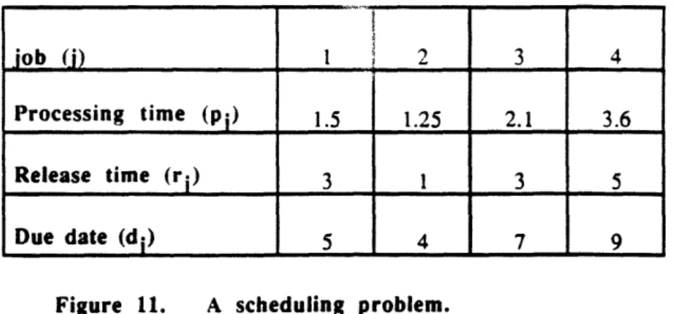
To illustrate the formulation of the feasible scheduling problem as a maximum flow problem, we shall use the scheduling data described in Figure 11.

Figure 11. A scheduling problem.

First, we rank all the release and due dates, rj and dj for all j, in ascending order and determine P < 2 JI

-1 mutually disjoint intervals of dates between consecutive milestones. Let Tkl denote the interval that starts at the beginning of date k and ends at the beginning of date 1+1. For our example, this order of release and due dates is 1, 3, 4, 5, 7, 9. We have five intervatls ^:,resented by T1.2, T3 3 , T4,4, T5,6 and

T7,8. Notice that within each interval Tk,,. the set of availa.:: .obs (that is, those released, but not yet

due) does not change: we can process all jobs j with rj < k and I + 1 in the interval.

We formulate the scheduling problem as a maximum flow problem on a bipartite network G as follows. We introduce a source node s, a sink node t, a node corresponding to each job j, and a node corresponding to each interval Tkl, as shown in Figure 12. We connect the source node to every job node j with an arc with capacity pj, indicating that we need to assign a minimum of pj machine days to job j. We connect each interval node Tki, to the sink node t by an arc with capacity (I-k+l)M, representing the total number of machine days available on the days from k to I. Finally, we connect a job node j to every interval node TkI if rj < k and dj > +1 by an arc with capacity (I-k+l) which represents the maximum number of machines that we can allot to job j on the days from k to I. We next solve a maximum flow problem on this network: the scheduling problem has a feasible schedule if and only if the maximum flow value equals jE J pj (alternatively, for every node j, the flow on arc (s, j) is pj). The validity of this formulation is easy to establish by showing a one-to-one correspondence between feasible schedules and flows of value equal to

jE

job () I I 2 3 4

Processing time (pi) 1.5 1.25 2.1 3.6

Release time (r.) 3 1 3 5

Figure 12. Network for scheduling uniform parallel machines.

Application 10. Tanker Scheduling Problem (Dantzig and Fulkerson [1954])

A steamship company has contracted to deliver perishable goods between several different origin-destination pairs. Since the cargo is perishable, the customers have specified precise dates (i.e., delivery dates) when the shipments must reach their destinations. (The cargoes may not arrive early r late.) The steamship company wants to determine the minimum number of ships needed to meet the delivery dates of the shiploads.

To illustrate a modeling approach for this problem, we consider an example with four shipments; each shipment is a full shipload with the characteristics shown in Figure 13(a). For example, as specified by the first row in this figure, the company must deliver one shipload available at port A and destined for port C on day 3. Figures 13(b) and 13(c) show the transit times for the shipments (including allowances for

loading and unloading the ships) and the return times (without a cargo) between the ports.

23 (a) C D A 3 2 B 2 3 (b) A B D

mJ

Figure 13. Data for the tanker scheduling problem.

We solve this problem by constructing a network shown in Figure 14(a). This network contains a node for each shipment and an arc from node i to node j if it is possible to deliver shipment j after completing shipment i; that is, the start time of shipment j is no earlier than the delivery time of shipment i plus the travel time from the destination of shipment i to the origin of shipment j. A directed path in this network corresponds to a feasible sequence of shipment pickups and deliveries. The tanker scheduling problem requires that we identify the minimum number of directed paths that will contain each node in the network on exactly one path.

(a)

Ship- Origin Desti. Delivery

ment nation date

1 Port A Port C 3

2 Port A Port C 8

3 Port B Port D 3

- - - -

-S_le

N

(b)

Figure 14. Network formulation of the tanker scheduling problem. (a) Network of feasible sequences of two consecutive shipments.

(b) Maximum flow model.

We can transform this problem into the framework of the maximum flow problem as follows. We split each node i into two nodes i' and i" and add the arc (i', i"). We set the lower bound on each arc (i', i"), called the shipment arc, equal to one so that at least unit of flow passes through this arc. We also add a source node s and connect it to the origin of each shipment (to represent putting a ship into service), and we add a sink node t and connect each destination node to it (to represent taking a ship out of service). We set the capacity of each arc in the network to value one. Figure 14(b) shows the resulting network for our example. In this network, each directed path from the source node s to the sink node t corresponds to a feasible schedule for a single ship. As a result, a feasible flow of value v in this network decomposes into schedules of v ships, and our problem reduces to identifying a feasible flow of minimum value. We note that the zero flow is not feasible because shipment arcs have unit lower bounds. We can solve this problem, which is known as the minimum value problem, in the following manner. We first establish a feasible flow in the network by solving a maximum flow problem. We then send flow from node t to node s until no more flow can be sent. The solution at this point is an optimal solution of the minimum flow problem.

Several other applications bear a close resemblence to the tanker scheduling problem and can be solved using the same technique. We next briefly introduce some of these applications.

Optimal coverage of sporting events. A group of reporters wants to cover a set of sporting events in an olympiad. The sports events are held in several stadiums throughout a city. We know the starting time of each event, its duration, and the stadium where it is held. We are also given the travel times between different stadiums. We want to determine the least number of reporters required to cover the sporting events.

Airline scheduling problem. An airline has p flight legs that it wishes to service by the fewest possible planes. To do so, it must determine the most efficient way to combine these legs into flight schedules. The starting time for flight i is aiand the finishing time is bi. The plane requires rij time to

return from the point of destination of flight i to the point of origin of flight j.

I i _______

Machine setup problem. A job shop needs to perform eight tasks on a particular day. We know the start and end times of each task. The workers must perform these tasks according to this schedule and so that exactly one worker performs each task. A worker cannot work on two jobs at the same time. We also know the setup time (in minutes) required for a worker to go from one task to another. We wish to find the minimum number of workers to perform the tasks.

The maximum flow problem arises in many other applications, including: (1) problem of representatives (Hall [1956]); (2) distributed computing on a two-processor model (Stone [19771); (3) the tournament problem (Ford and Johnson [19591); (4) police patrol problem (Khan [1979]); (5) nurse staff scheduling (Khan and Lewis [19871); (6) solving a system of equations (Lin [1986]); (7) statistical security

of data (Gusfield [1988], Kelly, Golden and Assad [19921); (8) minimax transportation problem (Ahuja

[1986]); (9) network reliability testing (Van Slyke and Frank [1972]); (10) maximum dynamic flows (Ford and Fulkerson [1958]); (11) preemptive scheduling on machines with different speeds (Martel [1982]); and (12) multifacility rectilinear distance location problem (Picard and Ratliff [1978]). The following papers describe additional applications of the maximum flow problem or provide additional references: Berge and Ghouila-Houri [1962]; McGinnis and Nuttle [1978], Picard and Queyranne [19821, Abdallaoui [1987], Gusfield, Martel and Femandez-Baca [19871, Gusfield and Martel [1989], and Gallo, Grigoriadis and Tarjan [1989].

5. MINIMUM COST FLOW PROBLEM

The minimum cost flow model is the most fundamental of all network optimization problems. This problem, described in Section 1, is concerned with determining a least cost shipment of a commodity through a network that will satisfy demands at certain nodes from available supplies at other nodes. This model has a number of familiar applications: the distribution of a product from manufacturing plants to warehouses, or from warehouses to retailers; the flow of raw material and intermediate goods through the various machining stations in a production line; the routing of automobiles through an urban street network; and the routing of calls through the telephone system. Minimum cost flow problems arise in almost all industries, including agriculture, communications, defense, education, energy, health care, manufacturing, medicine, retailing, and transportation. Indeed, minimum cost flow problems are pervasive in practice. In this section, by considering a few selected applications, we illustrate some of these possible uses of minimum cost flow problems.

Application 11. Leveling Mountainous Terrain (Farley [1980])

This application was inspired by a common problem facing civil engineers when they are building road networks through hilly or mountainous terrain. The problem concerns the distribution of earth from high points to low points of the terrain in order to produce a leveled road bed. The engineer must determine a plan for leveling the route by specifying the number of truck loads of earth to move between various locations along the proposed road network.

We first construct a terrain graph which is an undirected graph whose nodes represent locations with a demand for earth (low points) or locations with a supply of earth (high points). An arc of this graph represents an available route for distributing the earth and the cost of this arc represents the cost of per truck

load of moving earth between the two points. (A truckload is the basic unit for redistributing the earth.) Figure 15 shows a portion of the terrain graph.

I

Figure 15. A portion of the terrain graph.

A leveling plan for a terrain graph is a flow (set of truckloads) that meets the demands at nodes (levels the low points) by the available supplies (by earth obtained from high points) at the minimum cost (for the truck movements). This model is clearly a minimum cost flow problem in the terrain graph.

Application 12. Reconstructing the Left Ventricle from X-ray Projections (Slump

and Gerbrands 1982])

This application describes a minimum cost flow model for reconstructing the three-dimensional shape of the left ventricle from biplane angiocardiograms that the medical profession uses to diagnose heart diseases. To conduct this analysis, we first reduce the three-dimensional reconstruction problem into several dimensional problems by dividing the ventricle into a stack of parallel cross sections. Each two-dimensional cross section consists of one connected region of the left ventricle. During a cardiac catheterization, doctors inject a dye known as Roentgen contrast agent into the ventricle; by taking X-rays of the dye, they would like to determine what portion of the left ventricle is functioning properly (that is, permiuing the flow of blood). Conventional biplane X-ray installations do not permit doctors to obtain a complete picture of the left ventricle; rather, these X-rays provide one-dimensional projections that record the total intensity of the dye along two axes (see Figure 16). The problem is to determine the distribution of the cloud of dye within the left ventricle, and thus the shape of the functioning portion of the ventricle, assuming that the dye mixes completely with the blood and fills the portions that are functioning properly .

X-Ray ProjectlUM X-RAy ProJeatio Obrvable Projeclor Intenmitli

J

Inaenery rIntes ies 000226788875300

(a) (b)

Figure 16. Using X-Ray projections to measure a left 'ventricle.

We can conceive of a cross section of the ventricle as a p x r binary matrix: a 1 in a position indicates that the corresponding segment allows blood to flow and a 0 indicates that it doesn't permit blood to flow. The angiocardiograms gives the cumulative intensity of the contrast agent in two planes which we can translate into row and column sums of the binary matrix. The problem is then to construct the binary matrix given its row and column sums. This problem is a special case the feasible flow problem that we discussed in Application 6.

Typically, the number of feasible solutions for such problems are quite large; and, these solutions might differ substantially. To constrain the feasible solutions, we might use certain facts from our experience that indicate that a solution is more likely to contain certain segments rather than others. Alternatively, we can use a priori information: for example, after some small time interval, the cross sections might resemble cross sections determined in a previous examination. Consequently, we might attach a probability pij that a solution will contain an element (i, j) of the binary matrix and might want to

find a feasible solution with the largest possible cumulative probability. This problem is equivalent to a minimum cost flow problem.

Application 13. Optimal Loading of a Hopping Airplane (Gupta 1985] and

Lawania [1990])

A small commuter airline uses a plane, with a capacity to carry at most p passengers, on a "hopping flight" as shown in Figure 17(a). The hopping flight visits the cities 1, 2, 3, ..., n, in a fixed sequence. The plane can pick up passengers at any node and drop them off at any other node. Let bij denote the number of passengers available at node i who want to go to node j, and let fij denote the fare per passenger from node i to node j. The airline would like to determine the number of passengers that the plane should carry between the various origins to destinations in order to maximize the total fare per trip while never exceeding the plane capacity.

I' . ''- (a) U0000000000000 0 ougooooooogo 3 0000000 003 000000 11100 0 5 000001 1111100 7 0000011I111110 8 0000 111111i0 8 000 11 111 110 nn r .. . . ooooorooo oooo 000000000000000 0 , _{..-- __________ 1} I

I