HAL Id: hal-00107298
https://hal.archives-ouvertes.fr/hal-00107298
Submitted on 24 Jan 2021
HAL is a multi-disciplinary open access
archive for the deposit and dissemination of
sci-entific research documents, whether they are
pub-lished or not. The documents may come from
teaching and research institutions in France or
abroad, or from public or private research centers.
L’archive ouverte pluridisciplinaire HAL, est
destinée au dépôt et à la diffusion de documents
scientifiques de niveau recherche, publiés ou non,
émanant des établissements d’enseignement et de
recherche français ou étrangers, des laboratoires
publics ou privés.
Gravitation Wave Emission from Radio Pulsars
Revisited
T. Regimbau, J. A. de Freitas Pacheco
To cite this version:
T. Regimbau, J. A. de Freitas Pacheco. Gravitation Wave Emission from Radio Pulsars Revisited.
Astronomy and Astrophysics - A&A, EDP Sciences, 2000, 359, pp.242. �hal-00107298�
AND
ASTROPHYSICS
Gravitation wave emission from radio pulsars revisited
T. Regimbau and J.A. de Freitas PachecoObservatoire de la Cˆote d’Azur, B.P. 4229, 06304 Nice Cedex 4, France (regimbau,pacheco@obs-nice.fr) Received 3 February 2000 / Accepted 26 April 2000
Abstract. We report a new pulsar population synthesis based
on Monte Carlo techniques, aiming to estimate the contribution of galactic radio pulsars to the continuous gravitational wave emission. Assuming that the rotation periods of pulsars at birth have a Gaussian distribution, we find that the average initial pe-riod is 290 ms. The number of objects with pepe-riods equal to or less than 0.4 s, and therefore capable of being detected by an interferometric gravitational antenna like VIRGO, is of the or-der of 5100–7800. With integration times lasting between 2 and 3 yr, our simulations suggest that about two detections should be possible, if the mean equatorial ellipticity of the pulsars is
ε =10−6. A mean ellipticity an order of magnitude higher
in-creases the expected number of detections to 12–18, whereas
forε < 10−6, no detections are expected.
Key words: gravitational waves – stars: pulsars: general
1. Introduction
The first large wide-band gravitational interferometric anten-nas, the French-Italian VIRGO and the American LIGO, should be fully operational at the beginning of the next century. The expected sensitivity of these detectors in terms of the gravita-tional strain is of the order of h≈ 10−22 for short-lived, im-pulsive bursts, and h≈ 10−26for periodic “long-lived” sources for which integration times of about 107s are possible. Clearly, a major concern of these detectors is to understand and min-imize the sources of noise which define the sensitivity of the antenna, but the identification of a possible “standard” source (or sources), having a well defined waveform, is also a relevant problem in the context of the signal detection.
Among the possible candidates, it is expected that neutron stars, which are known to be quite abundant in the Galaxy, could rank among conspicuous emitters of gravitational waves (GW). Rotating neutron stars may have a time-varying quadrupole mo-ment and hence radiate GW, by either having a triaxial shape or a misalignment between the symmetry and the spin axes, which produces a wobble in the stellar motion (Ferrari & Ruffini 1969; Zimmerman & Szedenits 1979; Shapiro & Teukolsky
Send offprint requests to: T. Regimbau
1983; de Ara´ujo et al. 1994). Moreover, fast rotating proto-neutron stars may develop different instabilities such as the so-called Chandrasekhar-Friedman - Schutz (CFS) instability (Chandrasekhar 1970; Friedman & Schutz 1978), responsible for the excitation of density waves traveling around the star in the sense opposite to its rotation, or to undergo a transition from axi-symmetric to triaxial shapes through the dynamical “bar”-mode instability (Lai & Shapiro 1995). All these mechanisms are potentially able to emit large amounts of energy in the form of GW.
Continuous GW emission by the entire population of rotat-ing neutron stars, assumed to have small deviations from ax-isymmetry, raises the possibility of detecting their combined signals. The contribution of individual observed sources, like galactic pulsars, has been considered by Barone et al. (1988), Velloso et al. (1996), among others. However, detected radio pulsars constitute only a small fraction of the actual galactic population. Attempts to estimate the gravitational strain of the total pulsar population have been made by Schutz (1991), Gi-azotto et al. (1997, hereafter GBG97), de Freitas Pacheco & Horvath (1997), Giamperi (1998). Excepting Schutz (1991), all these authors proposed to detect the square of the gravitational strain, and the sidereal modulation of the integrated signal was examined by GBG97 as well by Giamperi (1998). In order to perform such an estimation, the actual distribution of the rota-tion periods must be known. The rotarota-tion period is a critical pa-rameter, because the gravitational strain depends on the square of the angular velocity. Unfortunately, the observed distribution does not necessarily reflect the real period distribution due to different selection effects present in all pulsar searches. GBG97 assumed for their estimate an (optimistic) average rotation pe-riod of 5 ms, which now seems a rather short value. If we exclude binary millisecond pulsars, which have probably been spun-up by accretion mechanisms, several observational facts indicate that population I pulsars are born with smaller rotation veloc-ities (Bhattacharya 1990). Moreover, several population syn-thesis calculations also suggest higher initial periods (Narayan 1987; Bhattacharya et al. 1992). Magnetic coupling between the proto-neutron star and the outer envelope could be an efficient mechanism for transferring angular momentum, so reducing the initial angular velocity. Proto-neutron stars are expected to be hot, with temperatures around 109K. In this situation,
depend-T. Regimbau & J.A. de Freitas Pacheco: Gravitation wave emission from radio pulsars revisited 243
ing on the viscosity, a rapidly rotating proto-neutron star may excite r-modes, emitting GW which decelerates considerably the star. According to computations by Andersson et al. (1999), this mechanism sets a limit around P≈ 20 ms for the fastest newly born neutron stars. However, it should be emphasized that this value is a function of the adopted (uncertain) viscosity law.
In the present work we revisit the problem of the contribution to the continuous GW emission from the pulsar population in-side the galactic disk. We estimate the actual period distribution by using population synthesis based on Monte Carlo methods, looking for the best pulsar population parameters by comparing our simulation results with data. Using the model population, we compute the gravitational strain for each pulsar emitting GW in the frequency band of VIRGO, the total square of the signal as well the amplitude modulation due to the sidereal motion. We show, in agreement with the expectations made by de Freitas Pacheco & Horvath (1997), that the signal is strongly domi-nated by a few fast pulsars and/or by the nearest ones. The plan of this paper is the following: in Sect. 2 we describe our popu-lation synthesis method; in Sect. 3 we present the properties of the simulated population; in Sect. 4 we estimate the contribution to the continuous gravitational strain of such a population and finally, in Sect. 5 we present our main conclusions.
2. The population synthesis 2.1. The rotation period evolution
The evolution of the rotation period of a neutron star, in the framework of the magnetic dipole model, is given by (Pacini 1968) P ˙P = 8π 2 3 µ2 Ic3sin 2α (1) whereµ = 1 2BR 3
p is the surface magnetic moment, B is the
magnetic field, Rp and I are respectively the radius and the
moment of inertia of the neutron star, c is the velocity of light
andα is the angle between the rotation axis and the magnetic
dipole. Integration of this equation with constantα gives the
rotation period evolution of the so-called standard model. In the absence of abrupt changes of the magnetic torque or of the internal structure of the star, solutions of Eq. (1) indicates a smooth increase of the rotation period with time. However, most pulsars do not slow down regularly, but display variations in their spin rates in the form of glitches (Shemar & Lyne 1996) and timing noise. An important aspect of glitches is the per-sistent increase of the spin-down rate following these events, which could be due to a sudden and permanent increase of the external torque (Link & Epstein 1997). In order to explain the glitches observed in the spin evolution of the Crab pulsar, Alpar & Pines (1993) suggested a reduction of the moment of inertia, induced by changes in the internal structure of the star. This would produce a spin-up of the star due to angular momentum conservation, but a decrease in the spin-down rate, contrary to observations. As the star spins down, it becomes less oblate, in-ducing stresses that may lead to starquakes if the yield strength
of the solid crust is exceeded. Starquakes may affect the braking mechanism if they are able to change the position of the mag-netic moment with respect to the rotation axis. If the structural relaxation after a starquake occurs asymmetrically about the ro-tation axis due, for instance, to magnetic stresses, the figure and spin axes may become misaligned. Under this condition, the star precesses and relaxes to a new equilibrium state, corresponding to a new orientation of the magnetic dipole with respect to the rotation axis. This possibility was examined in a recent work by Link et al. (1998). In their picture, a spin-down pulsar reduces its equatorial radius by shearing material across the equator and moving material along faults to higher latitudes. Such crustal motions may produce an increasing misalignment between the rotation and magnetic axes, providing a natural explanation for the observed increases in the spin-down rate following glitches in the Crab, PSR 1830-08 and PSR 0355+54.
The migration of the magnetic dipole fromm an initial angle
α to an orthogonal position with respect to the spin axis was also
considered by Allen & Horvath (1997). They showed that with such a variable torque, non-canonical braking indices may be explained. Here we adopt the scenario developed by Link et al. (1998), assuming that the magnetic dipole migrates from an arbitrary initial angle to a final orthogonal position in a timescale tα. For our present purposes, this migration is modeled by the
equation
sin2(α(t)) = 1 − n0e−t/tα (2)
We emphasize that this equation is not the result of any physical model, but only a phenomenological representation of the above picture, in the sense that a given pulsar born with an initial angle
α0 = acos(√n0), will reach an orthogonal configuration in a
timescaletα.
Combining Eqs. (1) and (2) and integrating, we obtain for the evolution of the rotation period
P = P0[1 + t τ0 − n0 tα τ0(1 − e −t/tα)]1/2 (3)
where P0is the initial rotation period andτ0= 4π32
Ic3
P2 0
B2R6 is the
magnetic braking timescale. Fort >> tαwe recover essentially
the standard model evolution. However, Eq. (3) allows one to explain the existence of objects with short periods and with a rel-atively small deceleration rate, which would be the consequence of a small initial misalignment between the magnetic and the spin axes, but not due to a small magnetic field strength. Note that in our picture these pulsars are young, in spite of having a large indicative age ts=2 ˙PP.
Another important parameter characterizing the evolution of the rotation period is the so-called braking indexN defined
as
N = ΩΩ¨˙
Ω2 (4)
For the standard magnetic dipole model, the expected brak-ing index isN = 3. However, the few pulsars with N measured
for the Crab,N =2.837 for PSR1509-58, N =2.04 for
PSR0540-69. The exceptionally low value for the Vela pulsarN = 1.40
was recently reported, suggesting that the braking torque is not due to a “pure” stationary dipole field (de Freitas Pacheco & Horvath 1997). From Eqs. (3) and (4), the predicted braking index for our model is
N = [3 − 2(ts
tα
)ctg2(α(t))] (5)
This equation indicates that for young pulsars with ages less thantαthe braking indexN may be less than three, tending to
the canonical value whent >> tα.
The angleα may vary “discontinuously” when the crust
sud-denly cracks or almost “continuously” as Eq. (2) suggest. It is worth mentioning that pulsars like PSR1509-58 and PSR0540-69 have not yet displayed any glitch activity even though their braking indices are less than the canonical valueN = 3. This
could be an indication that other braking mechanisms are oper-ative such as, for instance, anomalous electro-magnetic torques recently discussed by Casini & Montemayor (1998).
For the Crab pulsar, since the true age, the braking indexN
andtsare known, we can compute using the equations above
the dipole migration ratectgα ·dαdt , which is about 9.2×10⁻⁵ rad/yr for a solution where the present angle between the spin and the dipole axes is about 64o. From glitch data spanning a time interval of about 20 yr, Allen & Horvath (1997) find a migration rate 1.8×10⁻⁵ rad/yr, which is about five times smaller than the predicted value. However, as those authors re-marked, such a time interval is still very short and discrepancies should be expected when a comparison is performed between the migration rate derived from the average of few events and that obtained from a continuous variation model. For the other remaining three pulsars, the average “continuous” migration rate isctgα ·dαdt = 6.5×10⁻⁵rad/yr (Allen & Horvath 1997). These rates are comparable to within an order of magnitude, re-inforcing the idea of a common origin and giving some support to our adopted spin-down model.
2.2. The method
Initial spin periods and magnetic fields are important param-eters tracing the formation history of neutron stars and their interaction with the surrounding medium. The pulsar popula-tion study by Narayan (1987) raised the so-called “injecpopula-tion” problem, which would connect the initial period and magnetic field in the sense that slow born neutron stars would be associ-ated with high field strengths. Unfortunately, the ages of most pulsars are unknown and present measurements for estimating the period and its time derivative are insufficient in order to es-timate the initial field and spin period. In this case, methods of population synthesis can be useful tools to estimate statistical values of these parameters, assuming ad-hoc distribution laws. Moreover, the observed pulsar population is strongly dominated by luminous objects, and since the radio emission depends on the spin period as well as on the spin down rate, present sam-ples are biased, excluding long-period and high-field objects as
well as old and faint pulsars. Comparison with actual data re-quires the inclusion of these selection and observational bias in the generation of synthetic catalogs, which are more treatable when Monte Carlo techniques are employed.
In order to generate a synthetic sample of pulsars, we need to model: (a) their distribution in the Galaxy, (b) the initial param-eters affecting their evolution, (c) the effects of the interstellar medium in their detection and, (d) the sensitivity of a given survey.
The distribution in the Galaxy was modeled by assuming a constant birthrate until a maximum age tmax, considered as a
free parameter in our numerical experiments. The ratio between the total number Np of generate pulsars and tmax gives the
mean birthrate. For a given experiment, Np is the number of
input pulsars required to reproduce the number of objects in the data sample, when observational and selection constraints are imposed.
Pulsars are strongly concentrated in the galactic plane and their distribution along the z-axis can be represented by an ex-ponential law with a scale of height of about 100 pc. Some pre-vious studies suggest a possible correlation between the height above the galactic plane and age or magnetic field (Narayan & Ostriker 1990), but here we assume that the initial z-coordinate is a statistically independent variable. In the galactic plane, the density of pulsars probably decays exponentially, in the same way as population I objects. Recent galactic mass profile mod-els, based on infrared data, suggest a short distance scale of about 2.3 kpc (Ruphy et al. 1996); this was adopted in our nu-merical experiments. In order to compute heliocentric distances, the galactocentric distance of the sun was assumed to be 8.5 kpc. Some pulsars have significant proper motions, implying large initial velocities that must be taken into account when comput-ing distances, since they affect the orbital motion in the Galaxy. An isotropic Gaussian velocity distribution with 1-D velocity dispersion of 100 km s−1 (Lorimer et al. 1993) was adopted to simulate the pulsar kick velocity, but our results are not sig-nificantly changed if the velocity dispersion is increased up to 200 km s−1. Once the initial R and z coordinates for a given pulsar were established, if its kick velocity is zero, we assumed that the pulsar follows a circular orbit using the galactic rotation curve by Schmidt (1985). For non-zero kick velocity, the new energy and angular momentum of the orbit were computed and the object was settled in a new trajectory. The heliocentric dis-tance is computed after a time t (the age of the pulsar), taking into account the differential rotation between the sun and the pulsar. The present galactic coordinates (l, b) of the object are also computed, since these are required to establish if the pulsar should be included or not in the area of the sky covered by a given survey, as we shall see later.
In the present simulations we have assumed that the ini-tial rotation period of pulsars can be represented by a Gaussian distribution, characterized by a mean value P0and a dispersion
σP0. We have assumed that the break-up velocity is about 12000
rad s−1, thus pulsars generated with rotation periods less than 0.5 ms were not included in the simulated sample. These pa-rameters were allowed to vary in order to verify their effects on
T. Regimbau & J.A. de Freitas Pacheco: Gravitation wave emission from radio pulsars revisited 245
the results of different numerical experiments. A similar pro-cedure was adopted for the parameterτ0 (see, Eq. (3)), which
is related to the magnetic field of the pulsar, for which a log-normal distribution was assumed. Simulations by Bhattacharya et al. (1992) and by Mukherjee & Kembhavi (1997) suggest that the timescale for magnetic field decay is longer then the pulsar lifetime (τD > 100–160 Myr), thus we have assumed a
constant field in our numerical experiments. The initial angleα0
(or, equivalently, the value of n0) between the magnetic dipole
and the spin axes is calculated supposing a random distribution. Once these parameters are assigned for a given pulsar (tα is
kept fixed during a giving experiment), the period and the time derivative can be computed from Eq. (3).
The comparison between a simulated sample with actual data requires the evaluation of the expected radio flux density Sν at a given frequency (400 Mhz in general). To compute Sν,
one needs to know the distance and the luminosity of the pulsar. A theory able to predict the pulsar radio luminosity is still miss-ing, but the spin period and its time derivative are expected to be the main variables on which the radio power depends, since the magnetic field can be expressed in terms of these variables in the standard model. Different power laws have been suggested in the literature connectingP and ˙P (Lyne et al. 1975;
Stoll-man 1987; Emmering & Chevalier 1989). When these laws are compared with observational data a large dispersion is found, which can be explained by a bad understanding of the radio emission mechanism and/or by errors in the distance, estimates of which are derived by using the dispersion of radio waves through the interstellar plasma and by adopting a model for the electron density distribution inside the galactic disk. The ef-fects of the adopted luminosity law in numerical simulations were discussed by Lorimer et al. (1993), who concluded that, at the present time there appears to be no satisfactory model to account for observed pulsar luminosities.
The radio luminosity ought to be a decreasing function of the spin period, since slow pulsars missing in different surveys are probably too weak to be detected. Models assuming a radio lu-minosity proportional to the cube root of the spin-down rate lead to an inverse dependence on the period (Narayan 1987), while other proposed power laws indicate even higher exponents. In the present work, we have adopted a different empirical lumi-nosity law, imposing the following exponential fate on the radio emission
Lr= A ˙Pαe−γP (6)
The parameters in this relation were determined by an optimised fitting procedure, using the upgraded pulsar catalog of Taylor et al. (1993). If the luminosity is given in mJy.kpc2, and the period is in seconds, the resulting numerical values of the pa-rameters are: A=3.3×10⁷,α = 0.34 and γ = 1.02. These figures
are slightly different from those given by de Freitas Pacheco & Horvath (1997) because here we have used a larger sample in the fitting procedure.
The radio emission is not isotropic, implying that pulsars are not visible from all directions, and this imposes another constraint on their detectability. Following the approach used
by Emmering & Chevalier (1989), which will be adopted here, the beaming fraction of the sky covered by the pulsar emission cone is
f = (1 − cos θ) + (π2 − θ)sin θ (7)
where2θ is the aperture of the emission cone. Since short period
pulsars seem to have wider emission cones, we have adopted the beaming model proposed by Biggs (1990), which gives for the cone aperture
θ ≈ √6.2
P (8)
whereθ is in degrees and P is in seconds. It is worth mentioning
that the study by Rankin (1990) of a large sample of pulsars also indicates a variation ofθ inversely proportional to the square
root of the period.
Our data are a culled sample of 389 pulsars extracted from the catalog of Taylor et al. (1993), where only objects that have originated from population I stars and with all required param-eters measured were considered. Pulsars not included in any of the original surveys were also discarded. Since this catalog is a compilation of different catalogs covering specific sky areas and having a well defined sensitivity, the objects were distributed in sub-classes, according to the original surveys in which they were first detected.
Each simulated catalog to be compared with these data is prepared with the following prescriptions. For each pulsar gen-erated with a given set of initial parameters, we have followed its evolution in order to compute the presentP , ˙P values and
galactic coordinates, according to the scheme described above. Then the radio luminosity and the flux densitySν= Lr
d2 are
cal-culated, as well as the probability for the pulsar beam to cross the earth. The galactic coordinates define the survey (or surveys) included in the general catalog that covered this region. Then, we compare the expected flux density with the minimum de-tectable flux density of that survey through the relation (Dewey et al. 1984; Manchester et al. 1996)
Smin= A0(Tr+ Tsky)[
W
(P − W )]
1/2 (9)
where W is the observed (broadened) pulse width, Trand Tsky
are respectively the system and the sky background temperature in the considered line of sight. A0is a normalization constant,
defined as
A0=
(S/N )β
Ga√(np∆νtint)
(10) In this equation, Ga is the antenna gain, np is the number of
polarizations used, ∆ν is the receiver bandwidth, tint is the
integration time, S/N is the signal-to-noise ratio andβ is a
nu-merical factor, including other loss processes. The variation of the sky temperature with the galactic coordinates was estimated using the relation by Narayan (1987). The intrinsic pulse width Wewas assumed to be equal to 4% of the period (We=0.04P)
Table 1. Survey parameters
Survey Tr(K) τsam(ms) CDM(ms.pc−1.cm3) A0(mJy/K)
Arecibo 1 110 33 0.0094 0.038 Arecibo 2 90 0.6 0.0063 0.085 Arecibo 3-4 62 1.0(0.5) 0.0082(0.026) 0.02(0.032) Green Bank 1 170 33 0.28 0.30 Green Bank 2 30 33 0.28 0.13 Green Bank 3 30 4.0 0.035 0.18 Jodrell Bank 110 80 0.30 0.36 Molonglo 2 210 40 0.06(0.3) 0.17 Parkes 30 0.60 0.0125 0.19 s
dispersion and scattering, we follow the approach by Dewey et al.(1984) (see also Lorimer et al. 1993), writing for the relation between the observed and the intrinsic pulse width
W2= We2+ τsam2 + τsca2 + τDM2 (11)
whereτsamis the effective sampling time,τscais the broadening
due to diffusion through the interstellar medium andτDM is
the channel broadening. We have used the relation given by Bhattacharya et al. (1992) forτsca, namely,
τsca(ms) = 10−4.62+1.14log(DM )+ 10−9.22+4.46log(DM )(12)
where DM is the electron dispersion measure in the line of sight of the pulsar in pc.cm−3. For the channel broadening, we have used the relation
τDM(µs) = CDM.DM (13)
where, following Stokes et al. (1986)
CDM = 8.3
Bch(M Hz)
ν3(GHz) (14)
with Bchbeing the channel bandwidth andν the observing
fre-quency. Table 1 gives the main parameters characterizing the different catalogs adopted in our simulations. Note that values inside braces correspond to high latitude data.
Our procedure insures that the simulated catalog will have the objects distributed in the same proportion as in the global catalog, taking into account the specific sensibility and the sky area covered by each survey. The numerical experiments gener-ate objects according to these prescriptions until the simulgener-ated number of detectable pulsars is equal to the number in our data sample. For a given experiment, defined by a set of initial pa-rameters, the number of runs is comparable to the number of objects in the sample and the final result is a suitable average, in order to avoid statistical fluctuations.
For each experiment so defined, we have compared the re-sulting distributions with those derived from actual data. We searched for optimize the various input parameters that describe the pulsar population, controlling the fit quality throughχ2and Kolmogorov-Smirnov tests.
3. Properties of the simulated pulsar population
The possibility that the magnetic axis could migrate gives not only a possible explanation for the non-canonical braking index
-20 -15 -10 -5 0 5 10 15 20 -20 -15 -10 -5 0 5 10 15 20 Y ( kpc) X (kpc)
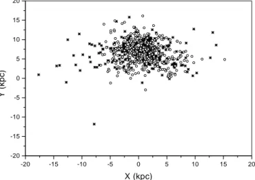
Fig. 1. Spatial distribution in the galactic plane (origin at the galactic center) of both observed (stars) and simulated (circles) populations of radio pulsars. The position of the sun is also indicated in the diagram. Table 2. Pulsar population properties
Parameters tmax= 24 Myr tmax= 100 Myr
P0(ms) 290±20 290±20
σP0(ms) 90±20 90±20
ln(τ0) (yr) 9.0±0.5 11.0±0.5
σln(τ0)(yr) 3.6±0.2 3.4±0.2
hlogBi (G) 12.4 12.1
observed in some pulsars, but also a mechanism affecting the
˙
P and age distributions. In general, objects with small
deceler-ation rates ( ˙P ≈ 10−16) are old and have low magnetic fields in the standard picture. In our scenario the magnetic torque controlling the deceleration rate, depends not only on the field strength but also on the angle between the dipole and the spin axes. Therefore, our simulated catalog contains some young objects born with a small misalignment between those axes, having a high field strength but a small deceleration rate. Un-fortunately, it is not possible to disentangle easily both situations and, as a consequence, the derived value of the dipole migration timescale tαhas a large uncertainty:tα= 10000±4000 yr. These
values imply migration rates spanning the interval (2–18)×10−5 rad/yr, which compare with rates derived by other authors (see Sect. 2.1).
The optimized parameters characterizing the distribution of the initial period and that of the magnetic braking timescaleτ0
are given in Table 2 for tmaxequal to 24 Myr and 100 Myr. These
parameters represent the best compromise able to fit adequately to data, the simulated distributions of period and its derivative, as well as the distribution of distances to the sun. Note that the parameters characterizing the Gaussian representing the initial distribution of rotation periods are not sensitive to the adopted value fortmax, but this is not the case for the parameterτ0.
In Fig. 1 we have plotted in the plane XY, which coincides with the galactic plane (the origin of the coordinates is placed at the galactic center), the observed pulsar population and our
T. Regimbau & J.A. de Freitas Pacheco: Gravitation wave emission from radio pulsars revisited 247 0 1 2 3 4 5 6 0,00 0,02 0,04 0,06 0,08 0,10 0,12 0,14 fr equency Period (s)
Fig. 2. Distribution of rotation periods. Bars represent observed binned data and filled circles indicate the result of our simulations. Error bars give the rmsd after averaging 500 numerical experiments.
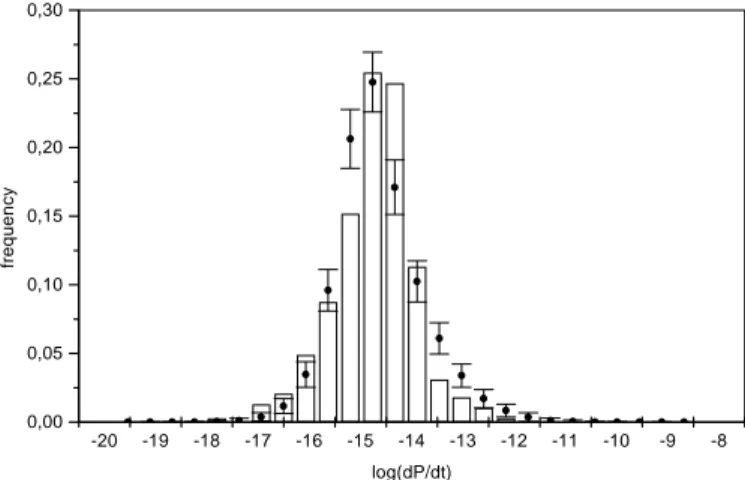
-20 -19 -18 -17 -16 -15 -14 -13 -12 -11 -10 -9 -8 0,00 0,05 0,10 0,15 0,20 0,25 0,30 fr equency log(dP/dt)
Fig. 3. Distribution of period derivatives. Symbols have the same mean-ing as in Fig. 1. 0 5 10 15 20 25 30 0,00 0,02 0,04 0,06 0,08 0,10 0,12 0,14 0,16 0,18 0,20 0,22 fr equency distance (kpc)
Fig. 4. Distribution of heliocentric distances. Symbols have the same meaning as in Fig. 1.
simulated population. The superposition of both populations is quite good, suggesting that selection effects were adequately taken into account by the model. In Fig. 2 we compare the ob-served period distribution with simulated data, where error bars
0,03 0,07 0,11 0,15 0,19 0,23 0,27 0,31 0,35 0,39 0,00 0,02 0,04 0,06 0,08 0,10 fr equency Period (s)
Fig. 5. Distribution of periods for all pulsars satisfying P<0.4 s.
correspond to the dispersion derived from five hundred experi-ments. Fig. 3 shows the comparison between observed and sim-ulated data for the period derivative, whereas Fig. 4 display both heliocentric distance distributions. These figures correspond to simulations withtmax= 24 Myr and they illustrate the fit quality.
The last line of Table 2 gives the average magnetic field of the simulated observed population, which is about 2.5×10¹²G, in agreement with values derived from a direct application of the “standard” pulsar model. However, the average field of the true or “unseen” population is one order of magnitude higher, namely, 2.5×10¹³G. Most of these high-field pulsar have rather long periods and thus are radio-quiet. The relevance of this high-field pulsar population in the context of magnetars will be dis-cussed in a forthcoming paper (Regimbau & de Freitas Pacheco 2000).
Our simulations indicate that the data are better explained if an initial distribution of periods is assumed instead of an unique (mean) initial value. Bhattacharya et al. (1992) assumed an ini-tial period equal to 100 ms, comparable with the average value derived from our simulations (290 ms). Models by Lorimer et al. (1993) are not directly comparable, since they have assumed a magnetic field decay with a timescale of 10 Myr. For the present purposes, we will focus our attention on the pulsar population with periods less than 0.4 s, which contributes to the contin-uum GW emission from the galactic disc. This upper bound is expected to be attained in a second phase of the VIRGO ex-periment. In spite of the bulk of the population having higher periods, the dispersion in the initial periods guarantees the exis-tence of objects in that frequency band. From our simulations, we predict about 60–90 (single) pulsars with P< 80 ms in the
Galaxy, a number not in contradiction with present data. The period distribution for pulsars satisfying the condition P< 0.4 s
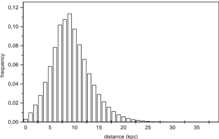
is shown in Fig. 5, and their heliocentric distance distribution is given in Fig. 6. The number of this sub-population is in the range 5100–7800, according to our simulations performed with tmaxequal to 24 Myr and 100 Myr respectively. The
contribu-tion of this populacontribu-tion to the gravitacontribu-tional strain is estimated in the next section.
0 5 10 15 20 25 30 35 0,00 0,02 0,04 0,06 0,08 0,10 0,12 fr equency distance (kpc)
Fig. 6. Distribution of heliocentric distances for the pulsar population satisfying P<0.4 s.
4. The gravitational strain 4.1. The equations
As we have mentioned above, pulsars could emit GW by having a time-varying quadrupole moment produced either by a slight asymmetry in the equatorial plane (assumed to be orthogonal to the spin axis) or by a misalignment between the symmetry and angular momentum axes, case in which a wobble is induced in the star motion. In the former situation the GW frequency is equal to twice the rotation frequency, whereas in the latter two modes are possible: one in which the GW have the same fre-quency as the rotation, and another in which the GW have twice the rotation frequency. The first mode dominates by far at small wobble angles while the importance of the second increases for large values.
Here we neglect the possible precessional motion and, in this case, the two polarization components of GW emitted by a rotat-ing neutron star are (Zimmerman & Szedenits 1979; Bonazzola & Gourgoulhon 1996)
h+(t) = 2A(1 + cos2i) cos(2Ωt) (15)
and
h×(t) = 4Acosi.sin(2Ωt) (16)
where i is the angle between the spin axis and the wave propa-gation vector, assumed to coincide with the line of sight,
A = G
rc4εIzzΩ
2 (17)
G is the gravitation constant, c is the velocity of light, r is the distance to The source,Ω is the angular rotation velocity of the
pulsar and the ellipticityε is defined as
ε = Ixx− Iyy
Izz
(18) with theIijbeing the principal moments of inertia of the star.
The detected signal by an interferometric antenna is
h(t) = h+(t)F+(θ, φ, ψ) + h×(t)F×(θ, φ, ψ) (19)
whereF+ andF× are the beam factors of the interferometer,
which are functions of the zenith distanceθ, the azimuth φ as
well as of the wave polarization plane orientation ψ. Notice
that the anglesθ and φ are functions of time due to the Earth’s
rotation, introducing a modulation of the signal. The explicit functions for the beam factors, taking into account the geo-graphic localization and the orientation of the VIRGO antenna were taken from Jaranowski et al. (1998).
Concerning the detection strategy, recall that the population derived from our simulations of potential GW emitters is in the range 5100 - 7800. In this case, according to the conclusions by GBG97, it becomes advantageous to search for individual detections instead of the total square amplitude. Here we have simulated both strategies. In the former case, the strain ampli-tude was calculated for each pulsar satisfying the condition P
< 0.4 s, using Eq. (19) and assuming a random orientation for
the inclination i of the spin axis as well for the orientation of the polarization angleψ. Since the signal is modulated at twice
the rotation frequency, in general much shorter than the sidereal period, we have assumed also a random phase for the relative orientation of the detector with respect to the equatorial coordi-nate system. In the other case, the procedure adopted to calculate the total square of the strain was the following: first, we have squared equ.(19) and then performed an average in the time in-tervalτ , satisfying the condition, 0.4 s < τ < one day. In this
case, the cross terms give a null contribution and we obtain
h2(t) = A2[2(1 + cos2i)2F2
+(t) + 8 cos2iF×2(t)] (20)
This equation was used to compute the contribution from all simulated objects satisfying P< 0.4 s, assuming again a random
orientation for i andψ.
4.2. The results
The main differences between the present approach and previ-ous calculations should be emphasized. Our procedure allows a more realistic estimate of the rotation period distribution, as well the number of pulsars able to contribute to the gravita-tional strain. Addigravita-tionally the spatial distribution of those pul-sars throughout the galactic disc changes for each simulation, although their average properties remaining constant. It is thus preferable to present the statistics of our numerical experiments, from which is possible to estimate the probability of having a signal above a given threshold.
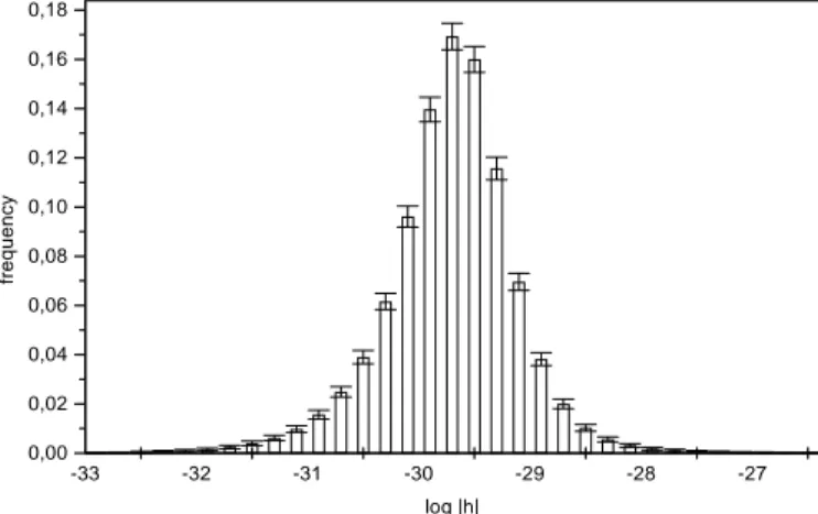
In Fig. 7 we give the statistics for the gravitational strain
h. For each experiment we have computed the distribution of
values of h and then averaged the results of 500 experiments. Error bars indicate the rmsd for each bin of thickness∆log(| h |) = 0.20. The resulting distribution can be represented quite well by a Laplace law, namely
L(x) = e(−2|x+29.7|) (21)
where x = log(| h |). This function corresponds to calculations performed with an ellipticityε = 10−6. For other values ofε, it
T. Regimbau & J.A. de Freitas Pacheco: Gravitation wave emission from radio pulsars revisited 249 -33 -32 -31 -30 -29 -28 -27 0,00 0,02 0,04 0,06 0,08 0,10 0,12 0,14 0,16 0,18 fr equency log |h|
Fig. 7. Distribution of the gravitational strain h for ε = 10−6. Error
bars indicate rmsd after averaging 500 numerical experiments.
-54 -52 -50 -48 -46 0,00 0,01 0,02 0,03 0,04 0,05 0,06 0,07 0,08 fr equency log (Hmax 2 )
Fig. 8. Distribution of the total h2 for ε = 10−6, corresponding to
7000 numerical experiments.
is enough to replace the constant in Eq. (21) by 23.7 log(ε). The
probability per pulsar to have a signal above x0is
p(x0) =
Z ∞
x0
L(x)dx (22)
For a continuous source, VIRGO (or LIGO) will be able to detect amplitudes of the order of h≈ 10−26, with integration times of about 2–3 yr. From the equation above and the population number estimated previously, one should expect to detect about 2 objects ifε = 10−6 or about 12–18 pulsars ifε = 10−5. If
the average ellipticity is smaller than 10−6, most of the objects will be below the detection threshold, at least for the present antenna sensibility.
In Fig. 8 we present the statistics for the square of the amplitude, resulting from the different spatial distribution of the pulsars in each numerical experiment. We emphasize that the amplitude of the signal is due essentially to a few pulsars, in agreement with the conclusions derived from the statistics of single objects and with the analytical study by de Freitas Pacheco & Horvath (1997). As a consequence, the sidereal modulation is not fixed by the galactic center-anticenter asymmetry, but by those few dominant objects. No typical modulation curve was obtained, since the relative positions of
these pulsars vary from experiment to experiment. Using the equations by GBG97 for the signal-to-noise ratio, one should expect to detect a signal ofh2 ≈ 10−45 with the presently
planned VIRGO sensibility. Our simulations indicate that, if
ε = 10−6a signal of such an amplitude has weak probability to
be detected (about 1/100) and signals of the required amplitude can only be obtained if the average pulsar ellipticity is of the order of 10−4.
5. Conclusions
Estimates of the GW emission from the total pulsar popula-tion in the Galaxy require knowledge of the period and distance distributions. Selection and detection bias are strong and popu-lation synthesis methods are necessary in order to model these effects,to recover the “true” population properties from the ob-served distributions.
Pulsars are probably born with a range of periods and mag-netic fields. Here we have assumed ad-hoc initial distributions for these parameters, which were optimized in order to repro-duce actual data. Our numerical experiments suggest that the mean initial period at the pulsar birth is equal to 290 ms, con-firming the conclusions of other simulations. Nevertheless, we predict about 60–90 single pulsars in the galaxy with periods less than 80 ms, as a consequence of the dispersion in the initial periods.
The pulsar population satisfying the condition P<0.4 s, able
to contribute to the GW emission within the pass-band of VIRGO, amounts to about 5100–7800 objects. These num-bers are considerably smaller than the estimate adopted by GBG97 (1.4×10⁵). Those authors assumed that the popula-tion with P< 0.4 corresponds to about 28% of the total
pop-ulation. The adopted fraction is that derived from cataloged pulsars. However, our simulations indicate that this fraction is only about 3.5%, exemplifying the consequences of the detec-tion bias present in all surveys.
VIRGO will be able to detect a gravitational strain ampli-tude of h≈ 10−26with three years of integration. Under these conditions, our simulations indicate 2 detections ifε = 10−6
and up to 12–18 detections if ε = 10−5. If the average
el-lipticity is smaller than 10−6, no detections are expected, at least with the presently planned antenna sensitivity. The total square amplitude resulting from this population is below the VIRGO threshold and a detectable signal would be produced only if the average ellipticity is at least of order of 10−4, a
value which seems to be excluded by a recent re-analysis of the magnetic and gravitational torques in some (observed) young pulsars (Palomba 1999).
We emphasize that the present results concern uniquely the radio pulsar population and the contribution of a binary mil-lisecond population to the continuous GW emission remains to be estimated. These simulations are more difficult,since the rotation period evolution has a complex history, including de-celerating and acde-celerating phases, which will be discussed in a future paper.
References
Allen M.P., Horvath J.E., 1997, MNRAS 287, 615
Alpar M.A., Pines D., 1993, in: Van Riper K.A., Epstein R.I., Ho C. (eds.), Isolated Pulsars. Cambridge University Press, p. 17 Andersson N., Kokkotas K., Schutz B.F., 1999, ApJ 510, 846 Barone F., Milano L., Pinto I., Russo G., 1988, A&A 203, 322 Bhattacharya D., 1990, in: Ventura J., Pines D. (eds.), Neutron Stars:
Theory & Observations, NATO ASI Ser. vol. 344, p. 103 Bhattacharya D., Wijers R.A.M.J., Hartman J.W., Verbunt F., 1992,
A&A 254, 198
Biggs J.D., 1990, MNRAS 245, 514
Bonazzola S., Gourgoulhon E., 1996, A&A 312, 675 Casini H., Montemayor R., 1998, ApJ 503, 374 Chandrasekhar S., 1970, PRL 24, 611
de Ara´ujo J.C.N., de Freitas Pacheco J.A., Horvath J.E., Cattani M., 1994, MNRAS 271, L31
de Freitas Pacheco J.A., Horvath J.E., 1997, PRD 56, 859
Dewey R., Stokes G.H., Segelstein D., Taylor J., Weisberg J., 1984, in: Reynolds S., Stinebring D. (eds.), Millisecond Pulsars, NRAO - Green Bank, p. 234
Emmering R.T., Chevalier R.A., 1989, ApJ 345, 931 Ferrari A., Ruffini R., 1969, ApJ 158, L71
Friedman J.L., Schutz B.F., 1978, ApJ 222, 281
Giazotto A., Bonazzola S., Gourgoulhon E., 1997, PRD 55, 2014 Giamperi G., 1998, astro-ph/9801019
Jaranowski P., Kr´olak A., Schutz B.F., 1998, gr-qc/9804014 Lai D., Shapiro S.L., 1995, ApJ 442, 259
Link B., Epstein R.I., 1997, ApJ 478, L91
Link B., Franco L.M., Epstein R.I., 1998, ApJ 508, 838
Lorimer D.R., Bailes M., Dewey R.J., Harrison P.A., 1993, MNRAS 263, 403
Lyne A.G., Ritchings R.T., Smith F.G., 1975, MNRAS 171, 579 Lyne A.G., Manchester R.N., Lorimer D.R., et al., 1998, MNRAS 295,
743
Manchester R.N., Lyne A.G., D’Amico N., et al., 1996, MNRAS 279, 1235
Mukherjee S., Kembhavi A., 1997, ApJ 489, 928 Narayan R., 1987, ApJ 319, 162
Narayan R., Ostriker J.P., 1990, ApJ 352, 222 Pacini F., 1968, Nat 219, 145
Palomba C., 1999, astro-ph/9912356 Rankin J.M., 1990, ApJ 352, 247
Regimbau T., de Freitas Pacheco J.A., 2000, in preparation Ruphy S., Robin A.C., Epchtein N., et al., 1996, A&A 313, L21 Schmidt M., 1985, in: van Woerden H., Allen R.J., Burton W.B. (eds.),
IAU Symp. 106, The Milk Way. Boston, Lancaster: Reidel, p. 75 Schutz B.F., 1991, in: Blair D.B. (ed.), The Detection of Gravitational
Waves, Cambridge University Press
Shapiro S.L., Teukolsky S.A., 1983, in: Black Holes, White Dwarfs and Neutron Stars. New York: Wiley
Shemar S.L., Lyne A.G., 1996, MNRAS 282, 677 Stollman G.M., 1987, A&A 178, 143
Stokes G.H., Segelstein D.J., Taylor J.H., Dewey R.J., 1986, ApJ 311, 694
Taylor J.H., Manchester R.N., Lyne A.G., 1993, ApJS 88, 529 Velloso W., Barone F., Calloni E., Di Fiori L., Grado A., Milano L.,
Russo G., 1996, Gen. Rel. Gr. 28, 613 Zimmerman M., Szedenits, 1979, PRD 20, 351