Predicting file lifetimes for data placement in multi-tiered storage systems for HPC

(1)

HAL Id: hal-03217669

https://hal.archives-ouvertes.fr/hal-03217669

Submitted on 7 May 2021

HAL is a multi-disciplinary open access

archive for the deposit and dissemination of

sci-entific research documents, whether they are

pub-lished or not. The documents may come from

teaching and research institutions in France or

abroad, or from public or private research centers.

L’archive ouverte pluridisciplinaire HAL, est

destinée au dépôt et à la diffusion de documents

scientifiques de niveau recherche, publiés ou non,

émanant des établissements d’enseignement et de

recherche français ou étrangers, des laboratoires

publics ou privés.

Predicting file lifetimes for data placement in

multi-tiered storage systems for HPC

Luis Thomas, Sebastien Gougeaud, Stéphane Rubini, Philippe Deniel, Jalil

Boukhobza

To cite this version:

Luis Thomas, Sebastien Gougeaud, Stéphane Rubini, Philippe Deniel, Jalil Boukhobza. Predicting

file lifetimes for data placement in multi-tiered storage systems for HPC. Workshop on Challenges and

Opportunities of Eﬀicient and Performant Storage Systems, Apr 2021, Online Event, United Kingdom.

pp.1-9, �10.1145/3439839.3458733�. �hal-03217669�

(2)

Predicting file lifetimes for data placement in

multi-tiered storage systems for HPC

Luis Thomas

luis.thomas@ensta-bretagne.org ENSTA Bretagne Lab-STICC, CNRS, UMR 6285 Brest, France

Sebastien Gougeaud

sebastien.gougeaud@cea.fr CEA Bruyères-le-Châtel, France

Stéphane Rubini

stephane.rubini@univ-brest.fr Univ. Brest Lab-STICC, CNRS, UMR 6285 Brest, France

Philippe Deniel

philippe.deniel@cea.fr CEA Bruyères-le-Châtel, France

Jalil Boukhobza

jalil.boukhobza@ensta-bretagne.fr ENSTA Bretagne Lab-STICC, CNRS, UMR 6285 Brest, France

Abstract

The emergence of Exascale machines in HPC will have the foreseen consequence of putting more pressure on the stor-age systems in place, not only in terms of capacity but also bandwidth and latency. With limited budget we cannot imag-ine using only storage class memory, which leads to the use of a heterogeneous tiered storage hierarchy. In order to make the most efficient use of the high performance tier in this storage hierarchy, we need to be able to place user data on the right tier and at the right time. In this paper, we assume a 2-tier storage hierarchy with a high performance tier and a high capacity archival tier. Files are placed on the high performance tier at creation time and moved to capacity tier once their lifetime expires (that is once they are no more accessed). The main contribution of this paper lies in the design of a file lifetime prediction model solely based on its path based on the use of Convolutional Neural Network. Re-sults show that our solution strikes a good trade-off between accuracy and under-estimation. Compared to previous work, our model made it possible to reach an accuracy close to previous work (around 98.60% compared to 98.84%) while reducing the underestimations by almost 10x to reach 2.21% (compared to 21.86%). The reduction in underestimations is crucial as it avoids misplacing files in the capacity tier while they are still in use.

CCS Concepts: • Information systems → Information stor-age systems;Storage management; Hierarchical storage management; Information lifecycle management;

ACM acknowledges that this contribution was authored or co-authored by an employee, contractor or affiliate of a national government. As such, the Government retains a nonexclusive, royalty-free right to publish or reproduce this article, or to allow others to do so, for Government purposes only.

Keywords: Data placement, Multi-Tier Storage, File lifetime, Convolutional Neural Network, Machine Learning, High Performance Computing, Heterogeneous Storage, Storage Hierarchy

ACM Reference Format:

Luis Thomas, Sebastien Gougeaud, Stéphane Rubini, Philippe De-niel, and Jalil Boukhobza. 2021. Predicting file lifetimes for data placement in multi-tiered storage systems for HPC. InWorkshop on Challenges and Opportunities of Efficient and Performant Stor-age Systems (CHEOPS ’21), April 26, 2021, Online, United Kingdom. ACM, New York, NY, USA, 9 pages. https://doi.org/10.1145/3439839. 3458733

1 Introduction

The amount of data generated in the world seems to grow exponentially, from 4 zetabytes in 2013 to an estimated 185 zetabytes in 2025 [4]. This trend will continue as new su-percomputers are already reaching the exaflop in AI driven workloads [37]. Storage has always been a performance bot-tleneck in High Performance Computing (HPC) [28][36][20]. In order to cope with the amount of data that Exascale ma-chines will produce, storage systems need to improve both in terms of capacity and speed (bandwidth and latency) [20]. Since no single storage technology is capable of fulfilling both those roles at a reasonable cost [13], we need to use a hierarchy of different storage technologies. The combined use of Flash-based drives, magnetic drives (HDD) and tapes is standard [24] in HPC systems. Memory class storage such as 3dX-point are expected to join the aforementioned hier-archy in production to partially fill the gap between DRAM and Flash [17][5].

The management of this hierarchy is a complex endeavour. Parallel distributed file systems such as Lustre [12] are used to manage the vast amount of disks and data across those disks. The standard architecture used in HPC is a three tier hierarchy [19] composed of clusters of Flash-based drives, magnetic drives and tapes each grouped together in storage

(3)

CHEOPS ’21, April 26, 2021, Online, United Kingdom Thomas and Gougeaud, et al.

nodes and managed by a parallel distributed file system or an object store such as DAOS [22]. Because the storage capacity available on the high performance tier is often an order of magnitude lower than that of the other tiers [24], the fastest tier of this hierarchy should only contain a subset of files for the time period during which they require such a performance.

In our work, we used a hierarchy of two tiers, a high performance tier and a capacity tier used for archival purpose. The aforementioned issue of data placement over the storage tiers can be translated in two main research questions: 1) when to store files in the performance tier and 2) when to move them to the capacity tier. Questioning about how data should be moved/scheduled from a tier to another is out of the scope of this paper, so is the prefetching issue.

Several state-of-the-art work solutions investigated the data placement of objects or files in high performance tiers [32] [35] [34]. They were mainly performed for hybrid stor-age systems composed of flash-based disks and magnetic drives. A large proportion of those studies such as [23] [3] relied on continuous system monitoring of I/O patterns [27] to infer the moment at which data should be placed in such tier and when they should be evicted. While those strategies performed well in terms of I/O performance, the exhaustive monitoring used makes them hardly usable in large produc-tion systems [15] [2]

In [25], the authors solely relied on file names to infer the time duration where files are accessed, thus reducing drastically the monitoring cost. In fact, they observed that in some CEA ( French Atomic Energy Commission) [10][6] supercomputers[7] [8], 45.80% of the files were never ac-cessed 10 seconds after their creation [25]. They defined the duration between the last access to a file and its creation time as the file lifetime. They used machine learning approaches to predict file lifetimes based only on their paths. Paths were chosen as input for two reasons: (1) the path of the file is known at creation time and (2) it often contains metadata about the user and/or the application that created it. With this prediction in hand, they placed each file in the high performance tier once created and moved it to the capacity tier when the file lifetime expires.

The performance of previous solution was measured ac-cording to two metrics: (1) the accuracy, it is defined as the percentage of lifetime predictions that are within an order of magnitude from the real value; (2) the under-estimation, defined as the percentage of predictions that are below the real lifetime value. This is particularly important as underes-timated file lifetime would result in a premature file eviction leading to a performance degradation. In this previous work, the authors used two Convolutional Neural Networks (CNN): (1) a CNN trained for accuracy (2) and another trained to produce the least amount of under-estimations, for that they used different cost functions. Then trade-offs were found.

In this paper, like previous work [25], we used the access path of a file to accurately predict when a file will last be accessed. While previous work used two Convolutional Neu-ral Network using two different loss functions, we propose to use a single Convolutional Neural Network using a cus-tom loss function in order to reduce the computing power necessary for a prediction. To achieve this, we designed the custom loss function to optimize the ratio between accuracy and under-estimations. The intuition behind the design of the custom loss function stems from multi task learning[16], we used the weighted average of the two loss functions used in previous work [25]. Our objective is to increase the ac-curacy of our predictions while maintaining a low level of under-estimations. We also used early-stopping to prevent overfitting.

Using a dataset of 5 millions entries from a production system at CEA and through several experiments we empir-ically found that the best weights/ratios between the two loss functions was around 0.2 for the loss function yield-ing high accuracy and 0.8 for the loss function yieldyield-ing low under-estimations. With this setting we were able to train our network to reach 98.60% accuracy while keeping under-estimations under 2.21%. In comparison previous work achieved 98.84% accuracy and 21.86% under-estimations us-ing their highly accurate loss function while the other loss function yielded 90.91% accuracy and 0.88% under-estimations. Our solution is also more flexible since we can tune the weights of the loss function to either favor high accuracy or low under-estimations.

We first go over the background of this study, by describ-ing the storage system used at CEA along with the software used to manage data life cycle. Then we describe the solution we designed. We evaluate and analyze our results. We then go over the related work and finally we conclude this paper with our final analysis and future work.

2 Background

This section introduces the overall system architecture con-sidered and sketched in Fig. 1. The first section describes the used HPC multi tiered storage system architecture rep-resented by the two storage servers in the top left corner of Fig. 1 (high performance and high capacity tiers). The sec-ond section introduces the Robinhood policy engine which is represented by the right side of Fig. 1, Robinhood is a software that provides fast access to file metadata in HPC storage systems.

2.1 The Storage Hierarchy in HPC

Scientific applications such as weather simulations, genomic sequencing or geoscience necessitate petabytes of storage for datasets and results. These data are archived and their results keep growing larger. Caching and prefetching strate-gies were put in place in order to speed up the process of

(4)

reading and writing to storage memory which is several or-ders of magnitude slower than main memory (DRAM) which is itself orders of magnitude slower than cache and CPU registers [18]. In order to get the best latency and through-put, a common solution is to use Flash-based drives as an intermediate between traditional magnetic drives and main memory [38] [4]. The use of tape is the final piece of the puzzle, as it is used to archive the data. Tapes have a latency of around 20 seconds or more [24]. Data stored on tapes does not consume any power which makes it an ideal solution for long term storage. Finally, tape as a technology has the best $/GB ratio and is a necessary technology to reach the exabyte at a feasible economic cost. As an example, 60% of the storage capacity of the TGCC [9], a CEA supercomputer, relies on tapes.

Figure 1. Simplified view of the system.

2.2 Robinhood Policy Engine

Robinhood Policy Engine [21] is a versatile tool to manage contents of large file systems, it is developed by the CEA [6]. It maintains a replicate of file system metadata in a database that can be queried at will. It makes it possible to schedule mass action on file system entries by defining attribute-based policies. Robinhood is linked to the file system through the changelog as shown on the right side of Fig. 1. It stores all metadata information about the file system in a SQL database which makes it possible to retrieve the state of the file system at any time. In a production system, this translates to millions of file entries, with their associated creation time, last access and last modification time. We used the data extracted from Robinhood in the proposed contribution.

3 Predicting file lifetime for data

placement

This section aims to describe the full scope of our contribu-tion, beginning with an overview of our solution inside the existing storage system. We explain how our training and validation data is processed and describe how our solution works.

Figure 2. View of the training process

3.1 Overall predicting system architecture

Our contribution consists in a file lifetime predicting system that takes as input file paths. Fig. 1 shows a simplified view of the existing data management system where our solution would be integrated. In the top right corner are Lustre [12] instances with 2 storage servers, those servers contain differ-ent media types. The one on the right is a metadata server, it contains metadata about the other Lustre file systems and is connected to them with a secondary network called "man-agement network" with lower latency and bandwidth than the High Performance Data Network. The applications are running on compute nodes which are not represented in this figure; applications are connected to the Lustre Storage Server through the High Performance Data Network.

On the right side of the figure, the block labeled "Robin-hood Policy Engine" [21] represents the software solution used to create migration policies between the different tiers. Robinhood is connected to the management network and reads metadata changes from the metadata server. This is represented by the "changelog reader" in the figure. These metadata changes are processed and stored in a database. The database then receives SQL queries to check the state of the file systems without having to contact the metadata server directly. An administrator can then create a policy by periodically checking the state of the file system through the Robinhood database; such policies include data migrations or purges.

Our solution would stand inside Robinhood and filters only the "File creation" events. The path of the file would be processed to generate a prediction of its lifetime. The prediction would then update the database entry related to the file. These predictions are to be used to create a data migration policy, the files with expired lifetimes would be

(5)

moved from high performance tier to capacity tier. In Fig. 1, this would translate in a migration from the SSD storage server (high performance tier) to the HDD storage server (capacity or archival storage), thus granting us more space for newly created files on the performance tier.

3.2 File lifetime training framework

In order to work, our machine learning solution has to be trained on real examples. Training is an iterative process, we refer to each training pass as an epoch. An epoch is defined as the number of times the neural network has processed the entire dataset.

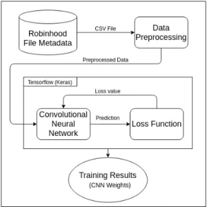
Fig. 2 shows the overall CNN training process. In our case, we used data from a production Robinhood database which had to be processed in order to remove fields with missing information. Those data are then transformed into a form that can be understood by a machine learning model. Then we design a model usingTensorflow and Keras to describe the layers of our Convolutional Neural Network and its hyper parameters such as the learning rate or the number of epochs. The model then goes through training and its performance is evaluated by a loss function (also referred to as cost function). The loss function is fundamental to the learning process as it will define how the neural network will change its param-eters. Previous work [25] used two different loss function to achieve either high accuracy or low under-estimations, we proposed a custom loss function using both of them. The three main components are described in the next sections. 3.3 Dataset processing

Data processing is a necessary part of our training system, its role is to transform the data from its source into a form that a machine learning solution can use. In our case we need fixed size inputs and file paths have variable sizes. We need also in this phase to define and normalize the metric of lifetime of files.

Our solution uses data from a production system at CEA [10]. They were extracted from a Robinhood Database used to monitor a production file system. Raw data extracted in this manner were the result of an SQL query, a Comma Sepa-rated Value (CSV) file that can be viewed as a table. This table contains fields with information on each file in the file system. We had access to the path, time of last access (or read), time of last modification (write), creation time and other associated metadata for each file.

The first step of data processing consists in processing each field of the CSV file in order to remove incoherent data such as a creation time being later than the last access time. The path column of each field was then converted from a character string of variable length (ex: /foo/bar/user/project/...) to a fixed size array of 256 integers. This size was chosen arbitrarily based on the commonly observed size of the paths. When the path was longer than 256 characters it was trun-cated from the start because we observed that the right part

of the path contains more relevant information such as the username, the file extension, etc. The transformed paths were considered as inputs for our CNN.

Figure 3. Lifetime distribution.

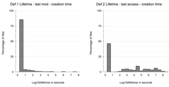
The second step of data processing is to define the life-time metric. There are three fields containing life-time infor-mation available in Robinhood: the creation time, the time of last access and the time of last modification. We came up with two possible definitions for the lifetime: 𝐷𝑒 𝑓 .1 = 𝑙𝑜𝑔10(𝑙𝑎𝑠𝑡 𝑚𝑜𝑑𝑖 𝑓 𝑖𝑐𝑎𝑡𝑖𝑜𝑛 𝑡𝑖𝑚𝑒 − 𝑐𝑟𝑒𝑎𝑡𝑖𝑜𝑛 𝑡𝑖𝑚𝑒) and 𝐷𝑒 𝑓 .2 = 𝑙𝑜𝑔10(𝑙𝑎𝑠𝑡 𝑎𝑐𝑐𝑒𝑠𝑠 𝑡𝑖𝑚𝑒 − 𝑐𝑟𝑒𝑎𝑡𝑖𝑜𝑛 𝑡𝑖𝑚𝑒). The decimal loga-rithm is used to discretize lifetime values. Fig.3 shows the distribution of lifetimes for each definition. The x-axis repre-sents the decimal logarithm (log10) of the lifetime in seconds and on the y-axis is the percentage of files close to that life-time. The bars represent the amount of files belonging to a certain lifetime slice in our dataset. It shows from left to right the lifetime distribution according to 𝐷𝑒 𝑓 .1 and 𝐷𝑒 𝑓 .2. We decided to use 𝐷𝑒 𝑓 .2, i.e. the time of last access minus the creation time because it contains more relevant information since the time of the last access can either be a write or a read while the time of last modification is always a write op-eration. This means that a prediction based on 𝐷𝑒 𝑓 .1 might evict some files before a read and thus would result in a per-formance penalty. So we defined the lifetime as the decimal logarithm of the difference between the time of last access and the creation time.

3.4 Model Architecture

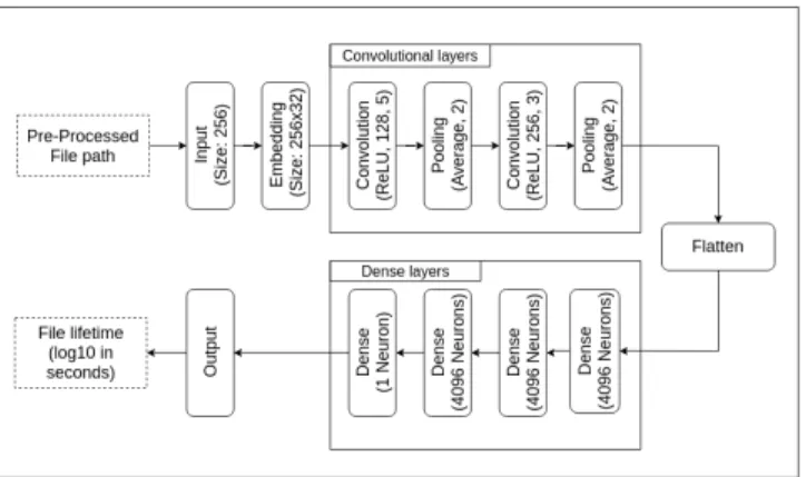
The CNN model architecture used in this paper was inspired from a previous work [25] which itself relied on [31]. A sim-plified representation of the model is shown on Fig.4. The architecture of the model is made of 12 layers: 1 input layer, 10 hidden layers and 1 output layer; Given the current trends in computer vision, this is a small CNN by its number of layers, but rather large in terms of parameters. For exam-ple, Inception v4 [33] contains 70 layers for 36.5 millions parameters while our model contains around 100 millions parameters (also referred as "weights"). We kept the same network layout as it performed adequately on this task in previous work [25] despite its number of parameters.

(6)

Figure 4. Simplified view of the model.

The training starts with the input layer, it fetches data from the dataset and passes it to the embedding layer.

Figure 5. Example of character embedding. 3.4.1 Embedding Layer. The embedding layer transforms the 256 bytes long input into a matrix of 256 by 32 floating numbers, we kept this size from previous work [25] and through multiple tries with different embedding values (16, 32, 48, 64). Fig. 5 shows an example with an 8 byte long input and an embedding size of 4. Each character is mapped to an array of floating numbers, these numbers change during training because they are learning parameters. We use em-bedding for two reasons: first, in order to leverage CNN, we need to transform the file paths into matrices of fixed size. Second because the alternative method to embedding, which is one hot encoding, takes too much space [30]. In our case one hot encoding would have multiplied the size of the input matrix by 3.

3.4.2 Convolutional Layers. The next layers are the con-volutional layers, they extract spatial data from the embed-ding layer that makes sense to the neural network. Theo-retically a convolutional layer produces a set of matrices containing features about the data it gets fed. Convolutional layers are defined by two parameters 1) the number of output matrices and 2) the size of the kernel used (128 and 5 for example). Pooling layers are used to reduce the dimension of

the input matrices of the next convolutional layer. Our model contains two convolutional layers and two pooling layers as shown in Fig. 4. The process of finding the right amount of layers is empirical and again was the result of experiments in previous work [25]. The output of a convolutional layer can be represented as a series of matrices containing features.

The layer that sits between the convolutional layers and the dense layers in Fig. 4 is the flatten layer, its role is to serialize the output of the last convolutional layer into a 1 dimensional array. Dense layers are defined by the number of neurons they contain. Each value in the output of the flatten layer is connected to each neuron in the dense layer. The dense layers are fully connected to each others. Almost all of the learning parameters are located in the dense layers, the weights in the previous layers (convolution, embedding) are negligible.

The output of the network takes the output of a dense layer made out of a single node and returns the lifetime of the file as previously defined. This model solves a regression problem since it returns a discrete value instead of probabilities to belong to a certain class.

3.5 Loss function

The goal of training a CNN like any other networks is to minimize a loss function. The loss function is used during training to compare the changes needed to be applied to the CNN in order to increase accuracy in the next iteration. It takes as inputs the predicted lifetime value and the real one. We present 4 loss function in this subsection, the first is one of the most commonly used in regression tasks, the following two were used by previous work [25] to train their CNNs. Finally we present our custom loss function which makes use of the two from previous work, thus the need to explain how they work.

One of the most commonly used loss function in regres-sion tasks isMean Squared Error or L2 [26]. MSE is the sum of squared distances between the real value and predicted values, it is defined as:

𝑀 𝑆 𝐸 = 1 𝑛 𝑛 Õ 𝑖=1 (𝑦𝑖 − ˜𝑦𝑖) 2

where 𝑦 represents the real value and ˜𝑦the predicted value. MSE should be used when the target values follow a normal distribution as this loss function would significantly penalize large errors. We observed that our data do not follow a normal distribution which explains why previous work [25] chose another loss function that is less affected by outliers in the data.

Previous work [25] usedlogcosh, which is another regres-sion loss function, in order to achieve high accuracy. It is defined as:

(7)

CHEOPS ’21, April 26, 2021, Online, United Kingdom Thomas and Gougeaud, et al. 𝐿= 1 𝑛 𝑛 Õ 𝑖=1 log(cos(𝑦𝑖−𝑦˜𝑖))

where 𝑦 represents the real value and ˜𝑦the predicted value. It works like MSE except that it is less affected by outliers in the dataset. Previous work [25] also usedquantile99 to achieve a low-level of under-estimations.quantile99 is the name given by [25] for thequantile loss function when the quantile is 0.99.Quantile loss function is defined as:

𝐿𝑞= 1 𝑛 𝑛 Õ 𝑖=1 max(𝑞 · (𝑦𝑖 − ˜𝑦𝑖), (𝑞 − 1) · (𝑦𝑖− ˜𝑦𝑖))

where 𝑞 represents thequantile value, 𝑦 the real value and ˜𝑦the predicted value. This loss function gives different values to over-estimations and under-estimations based on the quantile value. The closer the quantile value is to 1 the more it will penalize the under-estimations. The same is true for over-estimation, the closer the quantile is to 0 the more it will penalize over-estimations. A quantile value of 0.5 shows the same behavior as MSE.

The loss function used to train our model is a custom one. We realized through [16] that using the weighted average of quantile99 and logcosh allowed us to combine their properties while alowing for a higher flexibility thanks to the used weights. The custom loss function can be represented as:

𝑐𝑢𝑠𝑡 𝑜𝑚𝑙 𝑜𝑠𝑠() = 𝑤_𝑎· 𝑙𝑜𝑔𝑐𝑜𝑠ℎ() + 𝑤_𝑢· 𝑞𝑢𝑎𝑛𝑡𝑖𝑙𝑒99() where 𝑤𝑎+ 𝑤𝑢= 1. By modifying the value of the wieghts

𝑤𝑎and 𝑤𝑢we can either favor high accuracy or low

under-estimations.

The goal of this approach is to allow our solution to be adapted according to the system state, for instance, disk usage, I/O bandwidth, performance delta between tiers, the QoS required by the application, etc.

We evaluated different weight configurations in our ex-perimentation, that is :

(𝑤𝑎, 𝑤𝑢) ∈ {(0.5, 0.5), (0.4, 0.6), (0.3, 0.7), (0.2, 0.8), (0.1, 0.9)},

the results we obtained are discussed in Section 4.

4 Experimental Evaluation

This section covers the methodology used to evaluate our so-lution and the results we obtained against previous work [25]. We also discuss the flexibility of our solution by tuning the weights of our custom loss function.

4.1 Methodology

We trained the convolutional neural network in a docker container which had access to 4 Tesla V100 GPU. We used an optimization called mixed-precision in order to reduce the training time on GPU. We used Tensorflow 2 [1] to conduct all our experiments. With this optimization enabled, it took 2 hours to train our model (while the training lasted 4 hours

Table 1. Comparison of previous work against our solution evaluation metric logcosh quantile99 our solution

accuracy 98.84% 90.91% 98.60% under-estimations 21.86% 0.88% 2.21%

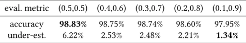
Table 2. Comparison of different weighted loss function for each (𝑤𝑎, 𝑤𝑢) value

eval. metric (0.5,0.5) (0.4,0.6) (0.3,0.7) (0.2,0.8) (0.1,0.9) accuracy 98.83% 98.75% 98.74% 98.60% 97.95% under-est. 6.22% 2.53% 2.48% 2.21% 1.34%

without mixed precision). In order to reduce training time we usedearly-stopping which monitors if the network is over-trained and if so stops the training.

The dataset we used contains 5 millions entries of real data from a production system in HPC. We pre-processed this dataset in order to keep only the path and the lifetime of each file using the method discussed in section 3. We used 70% of data for training and 30% for validation. The validation data were chosen randomly.

The metrics used to evaluate the performance of the net-work are the accuracy and the under-estimations.

4.2 Results

Table 1 shows the performance of logcosh and quantile99 against our solution, best values are emphasized. In this table, the weights of the loss function used for our solution were 0.2 forlogcosh and 0.8 for quantile99. While not reaching the accuracy oflogcosh our solution manages to be 7.5% more precise thanquantile99. On the other hand the number of under-estimations is almost divided by ten compared to logcosh.

By tuning the weights of our loss function we can fur-ther approach eifur-ther the accuracy oflogcosh or the under-estimations ofquantile99. Table 2 shows the influence of the weights of our loss functions on the metrics we observed, best performances are emphasized. A (0.5, 0.5) split between logcosh and quantile99 yields an accuracy of only 0.1% lower thanlogcosh alone while dividing underestimations by more than 3. In term of under-estimations, our solution is still outperformed by previous work usingquantile99 by 0.46% in the (0.1, 0.9) experiment. Overall we can observe that logcosh seems to have a bigger influence on the evaluation metrics thanquantile99. Accuracy declines slowly despite the proportion ofquantile99 getting larger. Since we defined an accurate prediction as a value an order of magnitude away from the real value then it is possible that the pre-dicted values are getting closer to leaving that interval as the proportion ofquantile99 increases. This would explain

(8)

the steep decline in precision between the (0.2, 0.8) and the (0.1, 0.9) experiments.

The conclusion we have drawn is that minimizing under-estimation is costly in terms of accuracy; Through multiple experiments, we were able to quantify the cost of reducing under-estimations in term of accuracy.

5 Related work

Predicting file lifetimes with Machine Learning was investi-gated in [25]. It was the main inspiration of this work. The authors used two machine learning algorithms, random for-est and a convolutional neural network (CNN). It showed that, on a dataset of 5 million entries, random forest was outperformed by the CNN both in terms of accuracy using logcosh and in terms of under-estimations using quantile99 as loss functions. Another observation they made from the data they recovered was that 45.80% of the files had a lifetime under 10 seconds.

eXpose [31] applies character embedding to URLs in a cybersecurity context. The embedding was used to train a Convolutional Neural Network to recognize malicious URLs. It is a highly influential work to the previously cited pa-per [25].

Learning I/O Access Patterns to improve prefetching in SSDs [11] leverages the use of Long Short-Term Memory (LSTM) which are an extension of Recurent Neural Networks to predict at firmware level (inside a SSD) which Logical Block Address will be used. In [14], the authors have eval-uated different learning algorithms, this time to model the overall performance of SSDs for Container-based Virtual-ization to avoid interference that would cause Service Level Objectives violations in a cloud environment

Data-Jockey [32] is a data movement scheduling solution that aims to reduce the complexity of moving data across a hierarchy of storage. It uses user-made policies to balance the load across all storage nodes and jobs. It has a view of the entire supercomputer and the end goal is to create a scheduler analog to SLURM for data migration jobs.

Archivist [29] is a data placement solution for hybrid em-bedded storage, it uses a neural network to classify files and outperforms baseline in latency access given certain conditions.

UMAMI [23] uses a range of different monitoring tools to capture a holistic view of the system. They show that their holistic approach allows them to analyse performance problems more efficiently.

The work presented in this paper follows and increments the approach in [25]. It upgrades the previous solution by 1) enhancing its performance in terms of accuracy and under estimations and 2) providing the administrator with a higher degree of flexibility by supplying a set of solutions allowing a trade-off between accuracy and under estimations.

6 Conclusions and Future Work

In this paper we propose a method to predict the lifetime of a file based on its path using a Convolutional Neural Net-work. We used data from a CEA production storage system to train our solution. We designed a custom loss function to get our Convolutional Neural Network to achieve a trade-off between high accuracy and low under-estimations. We then evaluated our solution against previous work [25], which used two loss functions: logcosh and quantile99. The results we obtained show that when using weights of 0.8 for quan-tile99 and 0.2 for logcosh our solution was able to reach an accuracy close to previous work using only logcosh (98.60% compared to 98.84%) while reducing the underestimations by almost 10 times to reach 2.21% (compared to 21.86%). Furthermore our solution is more flexible compared to pre-vious work since it allows system administrators to tune the weights of the loss function during incremental training to either favor high precision or low underestimations.

In future work we would like to investigate the use of our solution on a 3-tiered storage system (we used 2 tiers in this work). In such a context, we need to investigate new parameters to learn when to move data from one tier to another while still keeping the burden of monitoring low. Finally we would like to explore the use of a deeper CNN architecture in order to reduce the number of parameters, much like what is done in computer vision.

References

[1] Martín Abadi, Paul Barham, Jianmin Chen, Zhifeng Chen, Andy Davis, Jeffrey Dean, Matthieu Devin, Sanjay Ghemawat, Geoffrey Irv-ing, Michael Isard, Manjunath Kudlur, Josh Levenberg, Rajat Monga, Sherry Moore, Derek G Murray, Benoit Steiner, Paul Tucker, Vijay Vasudevan, Pete Warden, Martin Wicke, Yuan Yu, and Xiaoqiang Zheng. 2016. TensorFlow: A system for large-scale machine learn-ing. InProceedings of the 12th USENIX Symposium on Operating Systems Design and Implementation, OSDI 2016. USENIX, 265–283. https://doi.org/10.5555/3026877.3026899 arXiv:1605.08695

[2] Anthony Agelastos, Benjamin Allan, Jim Brandt, Paul Cassella, Jeremy Enos, Joshi Fullop, Ann Gentile, Steve Monk, Nichamon Naksineha-boon, Jeff Ogden, Mahesh Rajan, Michael Showerman, Joel Steven-son, Narate Taerat, and Tom Tucker. 2014. The Lightweight Dis-tributed Metric Service: A Scalable Infrastructure for Continuous Monitoring of Large Scale Computing Systems and Applications. InInternational Conference for High Performance Computing, Net-working, Storage and Analysis, SC. IEEE Computer Society, 154–165. https://doi.org/10.1109/SC.2014.18

[3] Djillali Boukhelef, Jalil Boukhobza, Kamel Boukhalfa, Hamza Ouarnoughi, and Laurent Lemarchand. 2019. Optimizing the cost of DBaaS object placement in hybrid storage systems.Future Genera-tion Computer Systems 93 (apr 2019), 176–187. https://doi.org/10.1016/ j.future.2018.10.030

[4] Jalil Boukhobza and Pierre Olivier. 2017.Flash Memory Integration (1st ed.). ISTE Press - Elsevier.

[5] Jalil Boukhobza, Stéphane Rubini, Renhai Chen, and Zili Shao. 2017. Emerging NVM: A Survey on Architectural Integration and Research Challenges.ACM Trans. Des. Autom. Electron. Syst. 23, 2, Article 14 (Nov. 2017), 32 pages. https://doi.org/10.1145/3131848

(9)

[6] CEA. 2020. CEA - HPC - Computing centers. Retrieved 2021-02-23 from http://www-hpc.cea.fr/en/complexe/computing-ressources.htm [7] CEA. 2020. CEA - HPC - TERA. Retrieved 2021-02-23 from http:

//www-hpc.cea.fr/en/complexe/tera.htm

[8] CEA. 2020. CEA - HPC - TGCC. Retrieved 2021-02-23 from http: //www-hpc.cea.fr/en/complexe/tgcc.htm

[9] CEA. 2020. CEA - HPC - TGCC Storage system. Retrieved 2021-02-23 from http://www-hpc.cea.fr/en/complexe/tgcc-storage-system.htm [10] CEA. 2020. English Portal - The CEA: a key player in technological

research. Retrieved 2021-02-23 from https://www.cea.fr/english/ Pages/cea/the-cea-a-key-player-in-technological-research.aspx [11] Chandranil Chakraborttii and Heiner Litz. 2020. Learning

I/O Access Patterns to Improve Prefetching in SSDs. In The European Conference on Machine Learning and Principles and Practice of Knowledge Discovery in Databases (ECML-PKDD). https://www.researchgate.net/publication/344379801_Learning_IO_ Access_Patterns_to_Improve_Prefetching_in_SSDs

[12] Sean Cochrane, Ken Kutzer, and L McIntosh. 2009. Solving the HPC I/O bottleneck: Sun™ Lustre™ storage system.Sun BluePrints™ Online 820 (2009). http://nz11-agh1.ifj.edu.pl/public_users/b14olsze/Lustre.pdf [13] Tom Coughlin. 2011. New storage hierarchy for consumer computers.

In2011 IEEE International Conference on Consumer Electronics (ICCE). 483–484. https://doi.org/10.1109/ICCE.2011.5722696 ISSN: 2158-4001. [14] Jean Emile Dartois, Jalil Boukhobza, Anas Knefati, and Olivier Barais. 2019. Investigating Machine Learning Algorithms for Modeling SSD I/O Performance for Container-based Virtualization.IEEE Transactions on Cloud Computing (2019). https://doi.org/10.1109/TCC.2019.2898192 [15] Richard Evans. 2020. Democratizing Parallel Filesystem Monitoring. In2020 IEEE International Conference on Cluster Computing (CLUSTER). 454–458. https://doi.org/10.1109/CLUSTER49012.2020.00065 [16] Ting Gong, Tyler Lee, Cory Stephenson, Venkata Renduchintala,

Suchismita Padhy, Anthony Ndirango, Gokce Keskin, and Oguz Elibol. 2019. A Comparison of Loss Weighting Strategies for Multi task Learn-ing in Deep Neural Networks.IEEE Access 7 (2019), 141627–141632. https://doi.org/10.1109/ACCESS.2019.2943604

[17] Takahiro Hirofuchi and Ryousei Takano. 2020. A Prompt Report on the Performance of Intel Optane DC Persistent Memory Module.IEICE Transactions on Information and Systems E103.D, 5 (May 2020), 1168– 1172. https://doi.org/10.1587/transinf.2019EDL8141 arXiv: 2002.06018. [18] Bruce Jacob, Spencer Ng, and David Wang. 2007. Memory Systems: Cache, DRAM, Disk. Morgan Kaufmann Publishers Inc., San Francisco, CA, USA.

[19] Kathy Kincade. 2019. UniviStor: Next-Generation Data Stor-age for Heterogeneous HPC. Retrieved 2021-02-23 from https://cs.lbl.gov/news-media/news/2019/univistor-a-next-generation-data-storage-tool-for-heterogeneous-hpc-storage/ [20] S Klasky, Hasan Abbasi, M Ainsworth, Jong Youl Choi, Matthew Curry,

T Kurc, Q Liu, Jay Lofstead, Carlos Maltzahn, Manish Parashar, Norbert Podhorszki, Eric Suchyta, F Wang, M Wolf, C.S. Chang, R. Churchill, and Stéphane Ethier. 2016. Exascale Storage Systems the SIRIUS Way. Journal of Physics: Conference Series 759 (Oct. 2016), 012095. https: //doi.org/10.1088/1742-6596/759/1/012095

[21] Thomas Leibovici. 2015. Taking back control of HPC file systems with Robinhood Policy Engine.International Workshop on the Lustre Ecosystem: Challenges and Opportunities (2015). arXiv:1505.01448 http: //arxiv.org/abs/1505.01448

[22] Zhen Liang, Johann Lombardi, Mohamad Chaarawi, and Michael Hennecke. 2020. DAOS: A Scale-Out High Performance Storage Stack for Storage Class Memory. InLecture Notes in Computer Sci-ence (including subseries Lecture Notes in Artificial IntelligSci-ence and Lecture Notes in Bioinformatics), Vol. 12082 LNCS. Springer, 40–54. https://doi.org/10.1007/978-3-030-48842-0_3

[23] Glenn K. Lockwood, Wucherl Yoo, Suren Byna, Nicholas J. Wright, Shane Snyder, Kevin Harms, Zachary Nault, and Philip Carns. 2017.

UMAMI: A recipe for generating meaningful metrics through holistic I/O performance analysis. InProceedings of PDSW-DISCS 2017 - 2nd Joint International Workshop on Parallel Data Storage and Data Intensive Scalable Computing Systems - Held in conjunction with SC 2017: The International Conference for High Performance Computing, Networking, Storage a. 55–60. https://doi.org/10.1145/3149393.3149395

[24] Jakob Lüttgau, Michael Kuhn, Kira Duwe, Yevhen Alforov, Eugen Betke, Julian Kunkel, and Thomas Ludwig. 2018. Survey of Storage Systems for High-Performance Computing.Supercomputing Frontiers and Innovations 5, 1 (April 2018), 31–58–58. https://doi.org/10.14529/ jsfi180103 Number: 1.

[25] Florent Monjalet and Thomas Leibovici. 2019. Predicting File Lifetimes with Machine Learning. InHigh Performance Computing, Vol. 11887 LNCS. Springer, 288–299. https://doi.org/10.1007/978-3-030-34356-9_23

[26] Feiping Nie, Zhanxuan Hu, and Xuelong Li. 2018. An investigation for loss functions widely used in machine learning.Communications in Information and Systems 18, 1 (2018), 37–52. https://doi.org/10.4310/ cis.2018.v18.n1.a2

[27] Hamza Ouarnoughi, Jalil Boukhobza, Frank Singhoff, and Stéphane Ru-bini. 2014. A multi-level I/O tracer for timing and performance storage systems in IaaS cloud. In3rd IEEE International Workshop on Real-Time and Distributed Computing in Emerging Applications (REACTION). IEEE Computer Society, 1–8.

[28] John K Ousterhout. 1990. Why Aren’t Operating Systems Getting Faster As Fast as Hardware?1990 Summer USENIX Annual Technical Conference (1990), 247–256.

[29] Jinting Ren, Xianzhang Chen, Yujuan Tan, Duo Liu, Moming Duan, Liang Liang, and Lei Qiao. 2019. Archivist: A Machine Learning As-sisted Data Placement Mechanism for Hybrid Storage Systems. In2019 IEEE 37th International Conference on Computer Design (ICCD). 676–679. https://doi.org/10.1109/ICCD46524.2019.00098 ISSN: 2576-6996. [30] Pau Rodríguez, Miguel Bautista, Jordi Gonzàlez, and Sergio Escalera.

2018. Beyond One-hot Encoding: lower dimensional target embedding. Image and Vision Computing 75 (05 2018). https://doi.org/10.1016/j. imavis.2018.04.004

[31] Joshua Saxe and Konstantin Berlin. 2017. eXpose: A Character-Level Convolutional Neural Network with Embeddings For Detecting Mali-cious URLs, File Paths and Registry Keys.arXiv:1702.08568 [cs] (Feb. 2017). http://arxiv.org/abs/1702.08568 arXiv: 1702.08568.

[32] Woong Shin, Christopher Brumgard, Bing Xie, Sudharshan Vazhkudai, Devarshi Ghoshal, Sarp Oral, and Lavanya Ramakrishnan. 2019. Data Jockey: Automatic Data Management for HPC Multi-tiered Storage Systems. In2019 IEEE International Parallel and Distributed Processing Symposium (IPDPS). 511–522. https://doi.org/10.1109/IPDPS.2019. 00061 ISSN: 1530-2075.

[33] Christian Szegedy, Sergey Ioffe, Vincent Vanhoucke, and Alexan-der A. Alemi. 2017. Inception-v4, inception-ResNet and the im-pact of residual connections on learning. In31st AAAI Conference on Artificial Intelligence, AAAI 2017. AAAI press, 4278–4284. https: //doi.org/10.5555/3298023.3298188 arXiv:1602.07261

[34] Bharti Wadhwa, Surendra Byna, and Ali Butt. 2018. Toward Trans-parent Data Management in Multi-Layer Storage Hierarchy of HPC Systems. In2018 IEEE International Conference on Cloud Engineering (IC2E). 211–217. https://doi.org/10.1109/IC2E.2018.00046

[35] Lipeng Wan, Zheng Lu, Qing Cao, Feiyi Wang, Sarp Oral, and Bradley Settlemyer. 2014. SSD-optimized workload placement with adap-tive learning and classification in HPC environments. In2014 30th Symposium on Mass Storage Systems and Technologies (MSST). 1–6. https://doi.org/10.1109/MSST.2014.6855552

[36] Wenguang Wang. 2004. Storage Management for Large Scale Sys-tems. Ph.D. Dissertation. CAN. https://doi.org/10.5555/1123838 AAINR06171.

(10)

[37] HPC Wire. 2020. Fujitsu and RIKEN Take First Place Worldwide in TOP500, HPCG, and HPL-AI with Supercomputer Fugaku. Retrieved 2021-01-25 from https://www.hpcwire.com/off-the-wire/fujitsu-and- riken-take-first-place-worldwide-in-top500-hpcg-and-hpl-ai-with-supercomputer-fugaku/

[38] Orcun Yildiz, Amelie Zhou, and Shadi Ibrahim. 2017. Eley: On the Effectiveness of Burst Buffers for Big Data Processing in HPC Systems. In2017 IEEE International Conference on Cluster Computing (CLUSTER). 87–91. https://doi.org/10.1109/CLUSTER.2017.73